Article

District Heating Load Prediction Algorithm Based on Feature Fusion LSTM Model

1
School of Artificial Intelligence, Hebei University of Technology, Tianjin 300401, China
2
School of Information and Engineering, Tianjin University of Commerce, Tianjin 300134, China
3
School of Energy and Environment Engineering, Hebei University of Technology, Tianjin 300401, China
4
School of International, Beijing University of Posts and Telecommunications, Beijing 100876, China
*
Author to whom correspondence should be addressed.
Energies 2019, 12(11), 2122; https://doi.org/10.3390/en12112122
Submission received: 28 April 2019 / Revised: 30 May 2019 / Accepted: 30 May 2019 / Published: 3 June 2019

Abstract

:
The smart district heating system (SDHS) is an important element of the construction of smart cities in Northern China; it plays a significant role in meeting heating requirements and green energy saving in winter. Various Internet of Things (IoT) sensors and wireless transmission technologies are applied to monitor data in real-time and to form a historical database. The accurate prediction of heating loads based on massive historical datasets is the necessary condition and key basis for formulating an optimal heating control strategy in the SDHS, which contributes to the reduction in the consumption of energy and the improvement in the energy dispatching efficiency and accuracy. In order to achieve the high prediction accuracy of SDHS and to improve the representation ability of multi-time-scale features, a novel short-term heating load prediction algorithm based on a feature fusion long short-term memory (LSTM) model (FFLSTM) is proposed. Three characteristics, namely proximity, periodicity, and trend, are found after analyzing the heating load data from the aspect of the hourly time dimension. In order to comprehensively utilize the data’s intrinsic characteristics, three LSTM models are employed to make separate predictions, and, then, the prediction results based on internal features and other external features at the corresponding moments are imported into the high-level LSTM model for fusion processing, which brings a more accurate prediction result of the heating load. Detailed comparisons between the proposed FFLSTM algorithm and the-state-of-art algorithms are conducted in this paper. The experimental results show that the proposed FFLSTM algorithm outperforms others and can obtain a higher prediction accuracy. Furthermore, the impact of selecting different parameters of the FFLSTM model is also studied thoroughly.

1. Introduction

The world’s largest district heating system (DHS) is located in China. This system needs to consume a large quantity of fossil energy, such as coal and natural gas, during winter. This leads to a serious air pollution problem and extremely harmful effects on human health and has, therefore, attracted the widespread attention of the whole society. The analysis of [1] suggests that the Huai River Policy, which had the laudable goal of providing indoor heat, had disastrous consequences for human health. Specifically, it led to an increase in inhalable particles (particulate matter 10, PM10), with concentrations of 46%, and reductions in life expectancies of 3.1 years, caused by elevated rates of cardiorespiratory mortality, in the north.
With the rapid development of urbanization and the increasing demand for comfortable heating by residents, the energy consumption of the DHS in China will increase significantly in the coming decades, and this will inevitably put significant pressure on energy supplements and environmental protection. Energy consumption is closely related to healthy economic development and daily human life. Combining the latest information technologies such as the Internet, the Internet of Things (IoT), and automation and communication technologies to develop a smart district heating system (SDHS) and to achieve energy saving has become one of the important goals of the DHS for the future of China. Thus, the heating load prediction algorithm has become one of the necessary conditions and key technologies for an intelligent heating system contributing to energy planning, operation regulation, realization of system energy saving, and emission reduction [2].
In recent years, the prediction of the energy consumption load has attracted the attention of many scholars, and many studies have been devoted to this purpose. Since the dataset collected by various sensors in the DHS has significant time series characteristics, and the heat transfer process has an evident delay and nonlinear characteristics; different nonlinear time series prediction algorithms can be used to solve the problem of heating load prediction. The previous studies on heating load prediction were mainly focused on the classical machine learning algorithms and their improvements, such as artificial neural networks (ANN), a support vector machine (SVM), support vector regression (SVR), and extreme learning machines (ELM).
In the early research period, Dotzauer [3] analyzed several factors affecting the heating load. The ANN has a good performance of linear fit, which is suitable for heating load prediction. Karatasou et al. [4] proposed an energy load prediction algorithm based on ANN. In order to improve the prediction performance of ANN, Boithias et al. [5] proposed a genetic algorithm (GA) to optimize ANN training parameters and model inputs. However, traditional ANNs are prone to over-fitting, difficult to initialize, and are difficult adjust the network parameters of. Thus, researchers gradually turned their attention to SVRs. Cai et al. [6] proved the superiority of an SVM in predicting building energy consumption. Zhang et al. [7] applied an SVR to accomplish the nonlinear regression prediction of building energy consumption. The theoretical analyzation for a prediction algorithm based on SVR was conducted by Fan et al. [8], who showed that the improvement strategies for SVR algorithms appeared in the short term. Hong [9] employed an immune algorithm (IA) to construct an SVR model to predict the annual electrical load in Taiwan. Ding et al. [10] proposed a short-term cooling load prediction algorithm for public buildings based on genetic algorithm–SVR (GA–SVR). Wang et al. [11] proposed a hybrid heating load prediction method based on particle swarm optimization and SVR. Al-Shammari et al. [12] proposed a hybrid prediction algorithm composed of an SVM and the firefly algorithm (FFA), which was named SVM–FFA and established seven heating load prediction models with different time scales. The FFA was employed to optimize SVM parameters to improve the prediction accuracy. Lee et al. [13] used a harmony search (HS) algorithm to determine the near-global optimal initial weights in the training of the model. The stratified sampling was used to sample the training data. A total of 25 HS–ANN hybrid models were tested with different combinations of DHS algorithm parameters. Dalipi et al. [14] proposed a data-driven supervised machine learning model to predict the heat load of buildings in a DHS. ELM was also employed for heating load prediction, as it is both simple and effective. Sajjadi et al. [15] proposed a short-term heat load prediction model of a DHS based on ELM. Roy et al. [16] applied a multivariate autoregressive (MVA) and an ELM hybrid model to predict a building’s thermal load.
However, traditional machine learning algorithms have certain limitations. Firstly, features need to be extracted manually, which makes it difficult to extract the features contained deep within the data. Then, the ability of nonlinear expression on the complex characteristic model is insufficient. Finally, the accuracy of the algorithm can reach a bottleneck and become difficult to improve.
After this, with the rapid development of deep learning (DL) technology in recent years, the related research based on DL algorithms has attracted the attention of many scholars. The recurrent neural networks (RNN) and long short-term memory (LSTM) are especially suitable for time series analysis and prediction based on the ability of feature extraction and nonlinear representation, which can automatically extract the deep features from the data and improve prediction accuracy. Kato et al. [17] innovatively proposed a heating load prediction algorithm based on RNN and achieved good prediction accuracy.
We compared the input factors to the literature related to heating load prediction. The results are shown in Table 1.
In addition to the heating system, the time series prediction problems based on deep learning have also attracted the attention of many scholars in other fields—solar irradiance prediction [19] building energy consumption [20], cooling load [21], electrical load [22,23,24,25,26,27], and wind power [28,29], for example.
Due to the fact that heating systems involve heat sources, heat exchange stations, primary pipe networks, secondary pipe networks, and thermal users, the nonlinearity and large delay characteristics of heat transfer make heating load prediction more complicated than for power systems. Fortunately, deep learning algorithms such as LSTM perform well in terms of time series feature extraction and nonlinear expression, which make them very suitable for heating load forecasting. However, the simple LSTM algorithm has a limited ability for historical features memory, and the large delay characteristic of heating systems makes the prediction possess a lower accuracy than that of the simple LSTM algorithm. Therefore, a feature fusion LSTM (FFLSTM) algorithm for the short-term prediction of a heating load is proposed in this paper, which combines the characteristic of proximity, periodicity, and trend, thus leading to a better performance compared with the-state-of-the-art algorithms. The best mean absolute percentage (MAPE) that can be achieved is 0.009, which is a dramatic improvement compared with the state-of-the-art algorithms.
In general, the main contributions of our paper are demonstrated as follows.
Firstly, the data characteristics and correlation of the heating system supervisory control and data acquisition (SCADA) system is analyzed, and three features that have a significant influence on the heating load prediction are found: The proximity, periodicity, and trend, which provide the basis for constructing the accurate heat load prediction model.
Secondly, layered prediction algorithm architecture for the heating load is designed based on the nonlinear and large delay characteristics of the heating system. The bottom layer is the LSTM prediction model with three different time scales, and the top layer establishes the feature fusion model.
Finally, according to different delay characteristics, six kinds of prediction mathematical models with different parameters are designed, and the experimental tests are compared. The delay characteristics suitable for the heating system are obtained, which provides support for the subsequent realization of energy-saving optimization prediction control.
The remainder of this paper is organized as follows: Section 2 analyzes the correlation characteristics of the original data and applies a Gauss filter to reduce the noise interference; Section 3 demonstrates the architecture and mathematical model of the proposed FFLSTM methodology in detail; Section 4 represents the experimental analysis and evaluation of the prediction performance; Section 5 is the conclusion.

2. Feature Analysis and Selection of Heating Load in SDHS

The FFLSTM algorithm needs to fully explore the unique characteristics of a heat load. In this section, two datasets, which were obtained the two stations of Xingtai Heating Company hourly heat load from 2017 to 2018, are used as examples. We analyzed the heat load features and selected the inputs of the models. For a better visualization, the first 10 days of data are plotted Figure 1 to show the performance of these three characteristics.
The three characteristics of the proximity, periodicity, and trend of the hourly data are considered in this paper. Figure 1 shows the periodic characteristics of the heating load data with two heat load fluctuations in 24 hours and a linear trend, shown as a red line. This is to ensure the thermal comfort of people after waking up in the morning, which involved increasing the secondary water supply temperature of the heat exchange station after 3:00 am in advance of them waking up. In the same manner, in order to ensure comfort heat levels after people get home from work every day, the secondary water supply temperature of the heat exchange station was increased after 15:00 pm. Therefore, the heat load of the heat exchange station has evident periodic characteristics. The heating load also has a significant correlation with the outdoor temperature, which leads to linear trend characteristics. From the perspective of the trend, in the early stage of heating, the heating load increases with the decrease in the room temperature; in the late cold stage, the heating load decreases with the increase of the outdoor temperature. However, due to the large hysteresis of the heating system, the daily energy consumption fluctuates differently.
According to thermodynamic heat conduction theory, the heat consumption of a heat exchange station is related to the secondary supply temperature, the secondary return temperature, and the flow rate. At the same time, due to the influence of thermal inertia and the meteorological factors of buildings, heat consumption is also related to historical heat consumption and outdoor temperature. The influencing factors are classified into the following two categories: Internal factors and external factors.
(1)
Internal factors:
  • Historical heat load (GJ)
  • Secondary supply temperature (supply temp for short) (°C)
  • Secondary return temperature (return temp for short) (°C)
  • Instantaneous flow rate (flow rate for short) (m3/h)
(2)
External factors:
  • Outdoor temperature (outdoor temp for short) (°C)
Figure 2 indicates a high correlation of the heat load with the characteristics of the historical heat load, outdoor temperature, second supply temperature, second return temperature, and instantaneous flow rate. Thus, these characteristics might be useful predictors of the dependent variable.

3. Methodology and Analysis

3.1. The Architecture of the Proposed FFLSTM

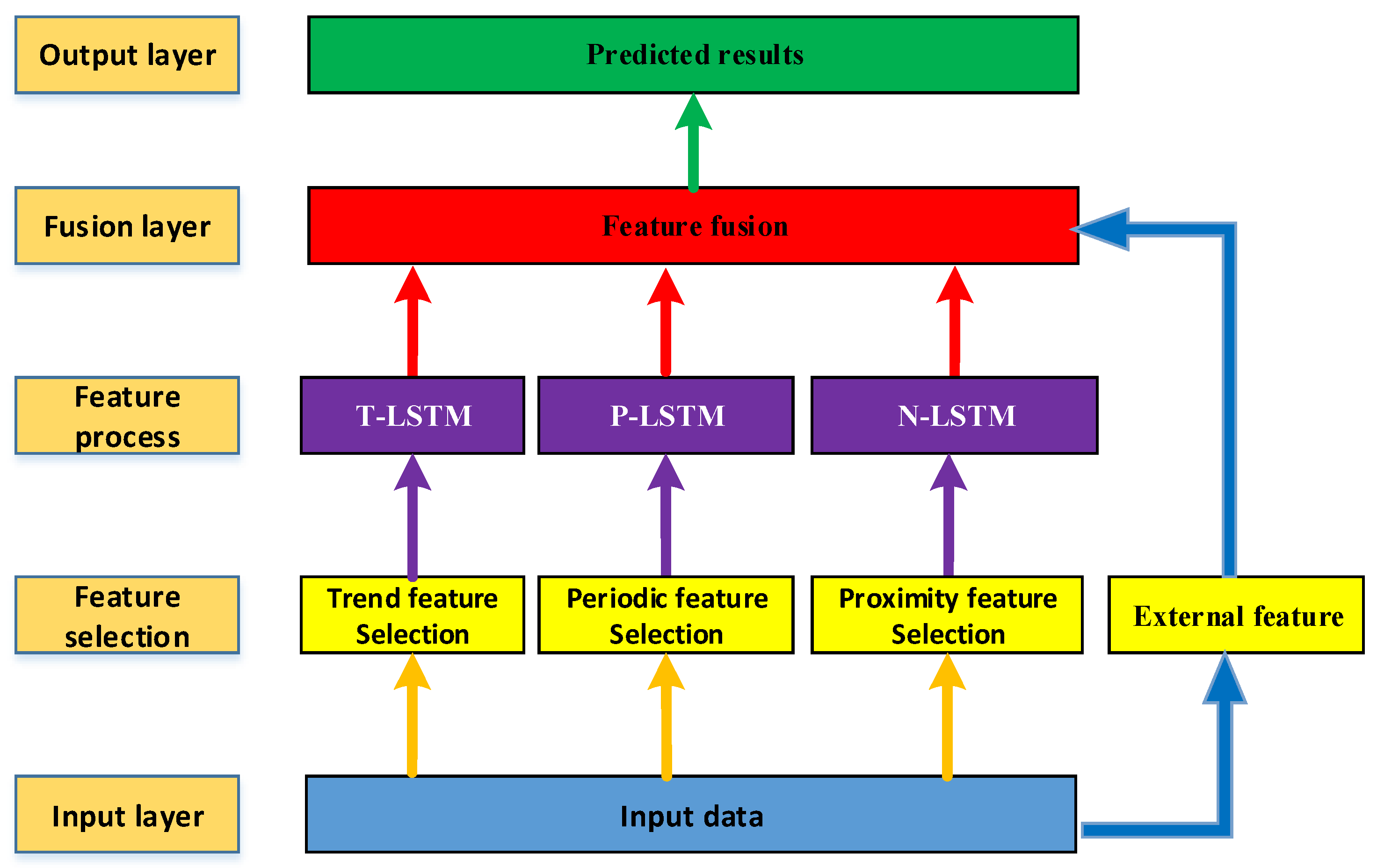
The intelligent district heating system is a complex nonlinear dynamic system, and the energy-saving regulation operation of the heat exchange station involves the characteristics and transmission delay of the primary network and the secondary network, the thermal inertia of the building, meteorological factors, and the personalized requirements of the terminal thermal users. Because the distance between each heat exchange station and the heat source is different and the fact that the buildings possess different energy saving characteristics, the historical dataset corresponding to the heat exchange station can essentially represent the comprehensive enclosure structural characteristics of buildings in the corresponding heating area. The prediction algorithm should automatically extract the corresponding delay characteristics and provide an accurate heating load prediction. This paper proposes a feature fusion integrated learning algorithm based on LSTM which can extract and process the characteristics of proximity, periodicity, and the trend of the heat exchange station load dataset and, then, obtain more accurate heating load prediction results after fusion processing so as to improve the accuracy of the energy saving regulation of heating. The overall architecture of the proposed FFLSTM model is presented in Figure 3.
As shown in Figure 3, the FFLSTM is a hierarchical structure with five layers. The input layer includes the time series of the secondary heating network and meteorology. The feature selection layer is used to select the characteristics of proximity, periodicity, and trend of the historical heat data. The feature processing layer uses LSTM to deal with three time-series with different time scale features. The three prediction models are called the N-LSTM, P-LSTM, and T-LSTM, and they deal with the three different data characteristics of proximity, periodicity, and trend, respectively. The feature fusion layer is used to process the prediction results of the N-LSTM, P-LSTM, and T-LSTM. At this stage, the external feature outdoor temperature is considered. Then, the prediction result of the FFLSTM is obtained in the output layer.

3.2. The Mathmatical Model of FFLSTM

The FFLSTM is a feature-based ensemble learning algorithm whose mathematical principles can be expressed as follows:
{ Q ^ h = f ( T h , Q ^ h N , Q ^ h P , Q ^ h T ) Q ^ h N = f 1 ( x h 1 , x h 2 , , x h i , , x h p ) Q ^ h P = f 2 ( x h 24 × 1 , x h 24 × 2 , , x h 24 j , , x h 24 q ) Q ^ h T = f 3 ( x h 24 × 7 × 1 , x h 24 × 7 × 2 , , x h 24 × 7 k , , x h 24 × 7 r )
where
Q ^ h denotes predicted heat consumption at the hour h;
Q ^ h N denotes the predicted heat load from proximity data at hour h;
Q ^ h P denotes the predicted heat load from the periodic data at hour h;
Q ^ h T denotes the predicted heat load from the trend data at hour h;
f indicates a predictive model of the fusion data;
f1 indicates a predictive model of the proximity data;
f2 indicates a predictive model of periodic data;
f3 indicates a predictive model of trend data;
x h i represents the proximity hourly input vector;
x h 24 j represents the periodic daily input vector;
x h 24 × 7 k represents the trend weekly input vector;
p = (1,2,…,24) represents the hours factor of the model;
q = (1,2,…,7) represents the days factor of the model; and
r = (1,2,3,4) represents the weeks factor of the model.
The three different time-scale feature vectors x h i , x h 24 j , and x h 24 × 7 k can be defined as shown in Equation (2), respectively:
{ x h i = ( T h i o , Q h i , T h i S , T h i R , F h i ) ( i = 1 , 2 , , p ) x h 24 j = ( T h 24 j o , Q h 24 j , T h 24 j S , T h 24 j R , F h 24 j ) ( j = 1 , 2 , , q ) x h 24 × 7 k = ( T h 24 × 7 k o , Q h 24 × 7 k , T h 24 × 7 k S , T h 24 × 7 k R , F h 24 × 7 k ) ( k = 1 , 2 , , r )
where
  • x h i represents the input vector composed of the outdoor temperature, heat consumption, secondary supply temperature, secondary return temperature, and instantaneous flow rate in the (h-i)th hour. The hours factor p = (1,2,…,24) represents the interval from the predicted time of the proximity input data, ranging from 1 to 24 h.
  • x h 24 j represents the input vectors such as the outdoor temperature, heat consumption, secondary supply temperature, secondary return temperature, and instantaneous flow in the (h-24j)th hour. The days factor q = (1,2,…,7) represents the interval from the predicted time of the periodic input data, ranging from 1 to 7 days.
  • x h 24 × 7 k represents the input vector of the outdoor temperature, heat consumption, secondary water supply temperature, secondary water return temperature, and instantaneous flow in the (h-24×7k)th hour. The weeks factor r = (1, 2, 3, 4) represents the interval from the predicted time of the trend input data, ranging from 1 to 4 weeks.
According to the analysis of section II, the factors of outdoor temperature (To), heat load (Q), secondary supply temperature (TS), secondary return temperature (TR), and instantaneous flow (F) are considered to build the predictive model for the purpose of achieving a more accurate prediction performance.
The SCADA system developed by our team collects these parameters once every 20 s and stores them in the database every 10 min. Thus, there are 24 groups of hourly datasets, which contain six measurement values for each parameter (hours group h = 1,2,3, …,24, internal index i = 1,2,…, 6). The original monitoring historical data are represented as the following:
T h , i o denotes the ith outdoor temperature measurement value at the hth hour;
T h , i S denotes the ith secondary supply temperature measurement value at the hth hour;
T h , i R denotes the ith secondary return temperature measurement value at the hth hour;
Fh,i denotes the ith instantaneous flow rate measurement value at the hth hour; and
Q h , i C denotes the ith cumulate heat load measurement value at the hth hour.
Because the heating system is a complex nonlinear system, and the heat transfer has a large delay, there will be a significant deviation in the real-time data collected by the SCADA system to predict the heating load. In general, hourly average measurements are required as the inputs to the prediction data. We preprocessed the original measurement data to form hourly statistical data.
{ T h o = 1 6 i = 1 n T h , i o T h S = 1 6 i = 1 n T h , i S T h R = 1 6 i = 1 n T h , i R F h = 1 6 i = 1 n F h , i Q h = Q ( h + 1 ) , 6 C Q h , 6 C
where,
T h o denotes the average outdoor temperature value at the hth hour;
T h S denotes the average secondary supply temperature value at the hth hour;
T h R denotes the average secondary return temperature value at the hth hour;
Fh denotes the average instantaneous flow rate value at the hth hour; and
Qh denotes the average heat load value at the hth hour.

3.3. Evaluation Criteria

In this paper, the root-mean-square error (RMSE), mean absolute error (MAE), and mean absolute percentage error (MAPE) were selected as the evaluation indices of the heat load prediction model, which are defined as:
{ R M S E = 1 n i = 1 n ( P i O i ) 2 M A E = 1 n i = 1 n | P i O i | M A P E = 100 n i = 1 n | P i O i P i |
where Oi and Pi represent the true value and predicted value of the heat load, respectively, and n represents the total number of the test samples.

4. Experiments and Discussion

4.1. System Background and Data Description

We have established a smart district heating system for the Xingtai Heating Company. With a heating area of about 16 million square meters with a total of 382 heat exchange stations, the real-time data acquisition and remote automatic control of the unattended heat exchange station were realized, and all data analysis and control strategies were completed in the monitoring data center. The datasets were collected from the heat exchange stations in Xingtai during the 2017–2018 heating season. The various sensors monitoring data were collected every 20 s and stored into the rational Microsoft SQL Server database every 10 min. There are 382 heat exchange stations and 120 days of each heating season, which ran from 15 October 2017 to 15 March 2018. Thus, the dataset size was 24hour/day × 120day × 6records/hour = 17,280 records for each substation, and the total records were about 17,280 × 382 = 6.6 million for the whole enterprise in one heating season, which can meet the requirement of the training and testing process of proposed FFLSTM algorithms.
The heat load predictions of each heat exchange station were independent of each other. A cross-validation method was used to verify the performance of the proposed algorithm. In our experiment, each dataset was split into a training dataset (70%), validation dataset (10%), and a testing dataset (20%).

4.2. Time Delay Factors Selection and Different Time-Scale Models

To determine the influence of the time delay characteristics on the heat load, correlation analysis was conducted on data of different time scales using Equation (5):
c o r r = i = 1 n ( x i x ¯ ) ( y i y ¯ ) i = 1 n ( x i x ¯ ) 2 i = 1 n ( y i y ¯ ) 2
where xi and yi represent two different variables, x ¯ represents the mean of xi, y ¯ represents the mean of yi, and corr represents the correlation between variables xi and yi.
The results of the correlation analysis are shown in Table 2. Here, p, q, and r represent proximity data, periodic data, and trend data intervals with the predicted time, respectively; the intervals of these three time characteristics are 1–5 h, 1–4 days, and 1–2 weeks, respectively.
Due to the different thermal inertia of the heating system and the different path-length from the heat source, the heat transfer has the characteristics of being non-linear and having a large delay. In addition, since the energy consumption of the heating system is significantly affected by meteorological factors, the time series data collected from the sensor cannot directly and accurately describe such complex factors.
To better extract the nonlinear time delay characteristics of the physical heating pipe network, we chose the time intervals (p = 1, 2, 3; q = 1, 2, and r = 1) based on the analysis the correlation of the characteristics of the original data shown in Table 2.
In this paper, a total of six different models are defined; this is shown in Table 3.

4.3. Parameter Selection and Performance Evaluation

In order to achieve the optimal prediction performance of the heat load model, the parameters of the LSTM network need to be selected in advance. In this paper, the selection of parameters of an LSTM model was based on the proximity data, and the initial parameters are shown in Table 4.
To determine the optimal value of these parameters for the experiments, every candidate is tested according to the sequence of learn_rate, batch_size, time_step, hide unit, and iter_count. The best performance of each parameter is taken as the optimal selection based on the previous experimental results.
As is shown in Table 5, when learn_rate is used as a single regulation variable, the best result is obtained, 0.002; learn_rate = 0.002 was used in the experiment and in the subsequent experiments. When batch_size was adjusted, the results obtained were not as good as those under learn_rate = 0.002 and batch_size = 20. Therefore, when time_step was used as a single variable, the parameter batch_size was still selected as 20.
The final selected experimental parameters are shown in Table 6. In order to ensure consistency, each LSTM model used the same parameters, which are shown in Table 6, in the entire fusion algorithm.

4.4. Compared with the Base LSTM Models

The integrated learning approach uses a series of independent models for prediction and then combines them to integrate a model. It can generate better prediction results. A single model sometimes only obtains local optimal results or over-fitting; therefore, the practice of combining multiple models can improve accuracy. The basic models in the FFLSTM feature processing layer are independent of each other. To achieve a better integration effect for determining the FFLSTM, the prediction results of the FFLSTM are compared with those of the three basic models, which are shown in Table 7.
In Table 7, the N-LSTM, P-LSTM, and T-LSTM represent LSTM proximity prediction, periodic prediction, and LSTM trend prediction, respectively. It can be seen that, in station A and station B, the N-LSTM shows better prediction results compared to those of P-LSTM and T-LSTM. This also indicates that the heating load of the heat exchange station is more correlated with the recent historical data of influential factors, such as the heat load and outdoor temperature. The FFLSTM obtained the highest prediction accuracy after the correction of periodicity and trend.

4.5. Compared with Other Algorithms

To evaluate the heat load performance of the proposed FFLSTM algorithm, we compared it with the state-of-the-art algorithms which are widely used in the forecasting field, such as traditional LSTM, back propagation (BP), SVR, a regression tree (RT), random forest regression (RFR), gradient boosting regression (GBR), and extra trees regression (ETR). The radial kernel function (RBF) was used in SVR for this paper; it can map a sample to a higher dimensional space and is suitable for training and testing with moderate data samples. The sigmoid activation function was used for BP. The size of the hidden layer and the number of iterations in the gradient descent loop of BP were 3 and 20,000, respectively.
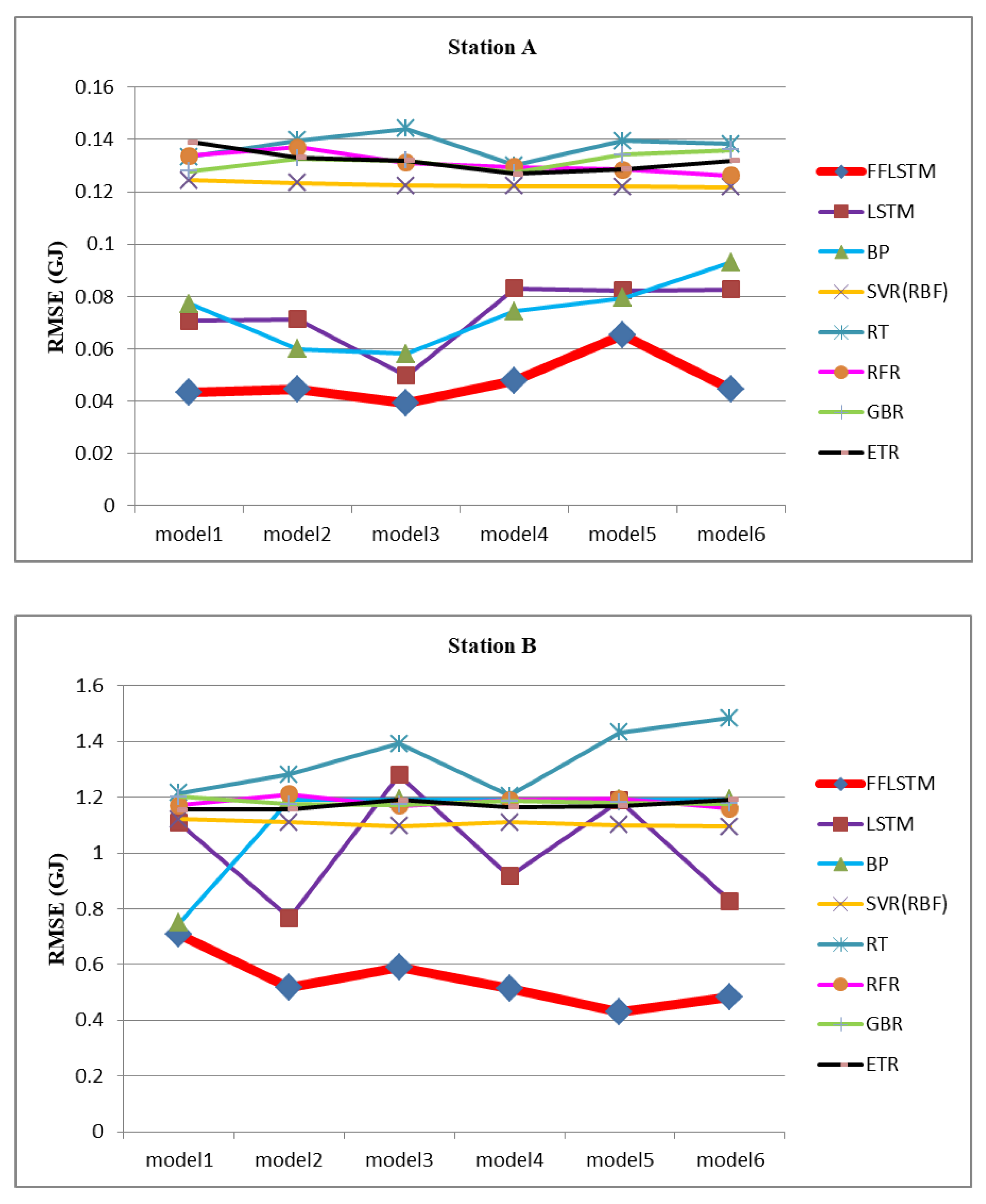
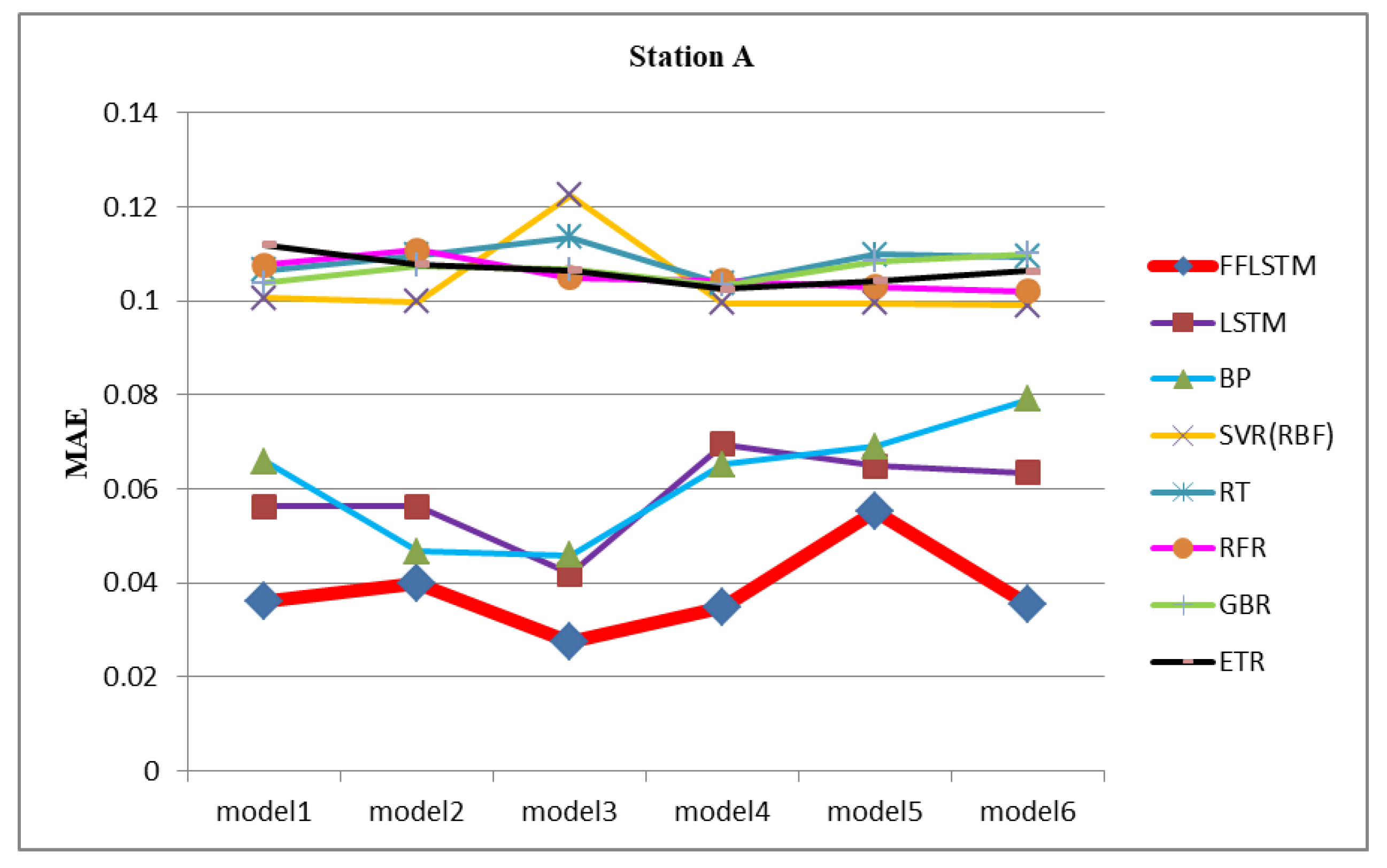
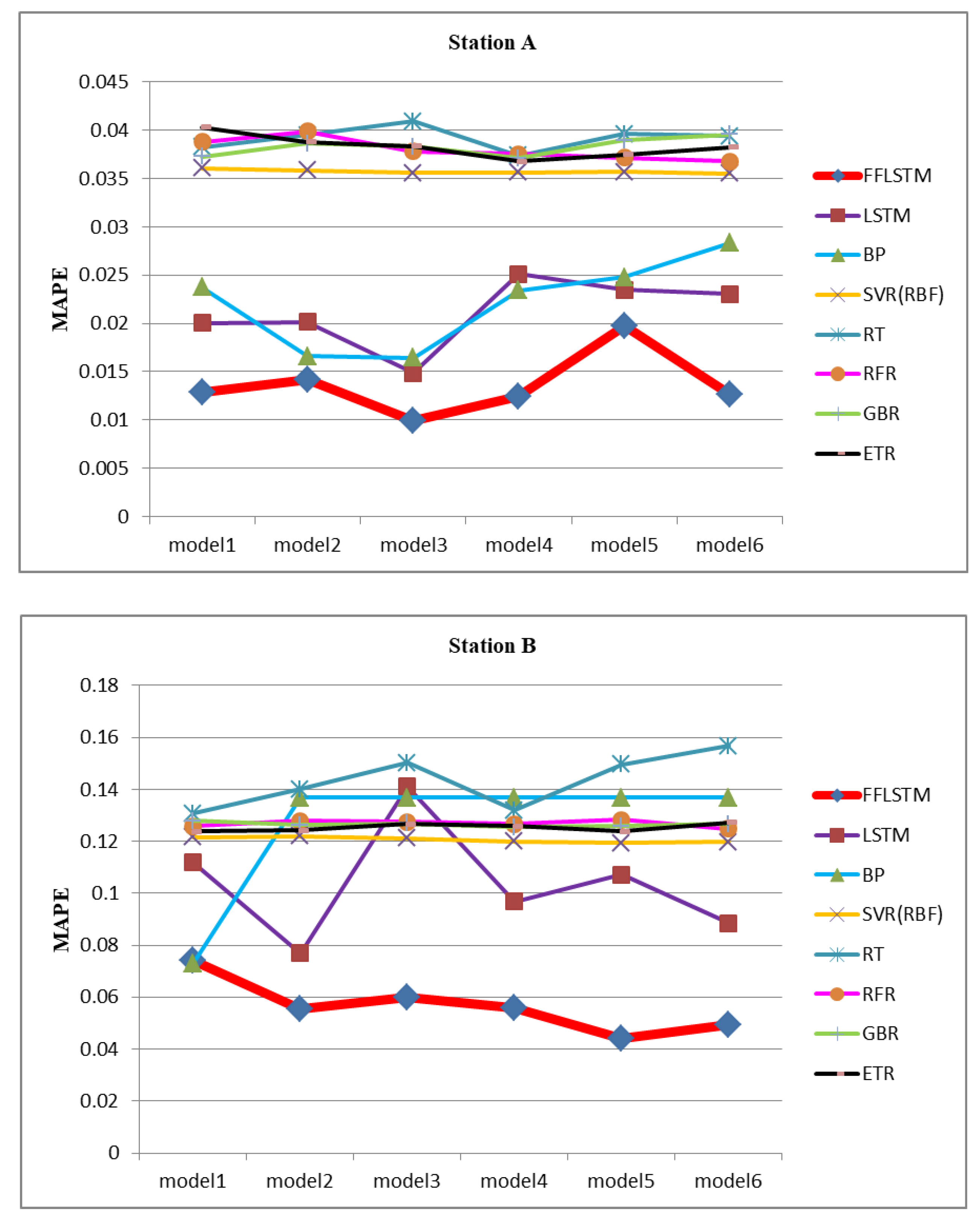
In order to prove the superiority of the proposed FFLSTM, the datasets of the two heat exchange stations were used to validate the model. The RMSE, MAE, and MAPE of station A and station B are shown in Figure 4, Figure 5 and Figure 6, respectively. In order to compare the prediction performance of different heat exchange stations in the same dimension for convenience, the normalized MAPE was selected as the main index parameter, and MAE and RMSE were selected as the auxiliary index parameters. Comprehensive experiments have shown that the FFLSTM has the best predictive power on both datasets. RMSE, MAE, and MAPE are smaller than the other comparison algorithms.
Table 8 lists the RMSE, MAE, and MAPE values of the proposed algorithm and the state-of-the-art comparison algorithms. Table 8 shows that the performance of the FFLSTM was optimal in the models. The RMSE, MAE, and MAPE of heat exchange station A reached 0.03 GJ, 0.02 GJ, and 0.009 GJ, respectively. The three evaluation indexes are significantly improved compared with other algorithms. The prediction accuracy of station A was above 98%, and station B was above 92%. Because the energy consumption prediction of heat exchange station B uses the network parameters trained by historical data of heat exchange station A, the prediction accuracy of heat exchange station B was slightly lower but also reached over 92%. This shows that the FFLSTM algorithm also has a good generalization ability. We chose the average of the six mode prediction results as the final prediction value, as shown in Table 9.

4.6. System Verification and Energy Saving Analysis

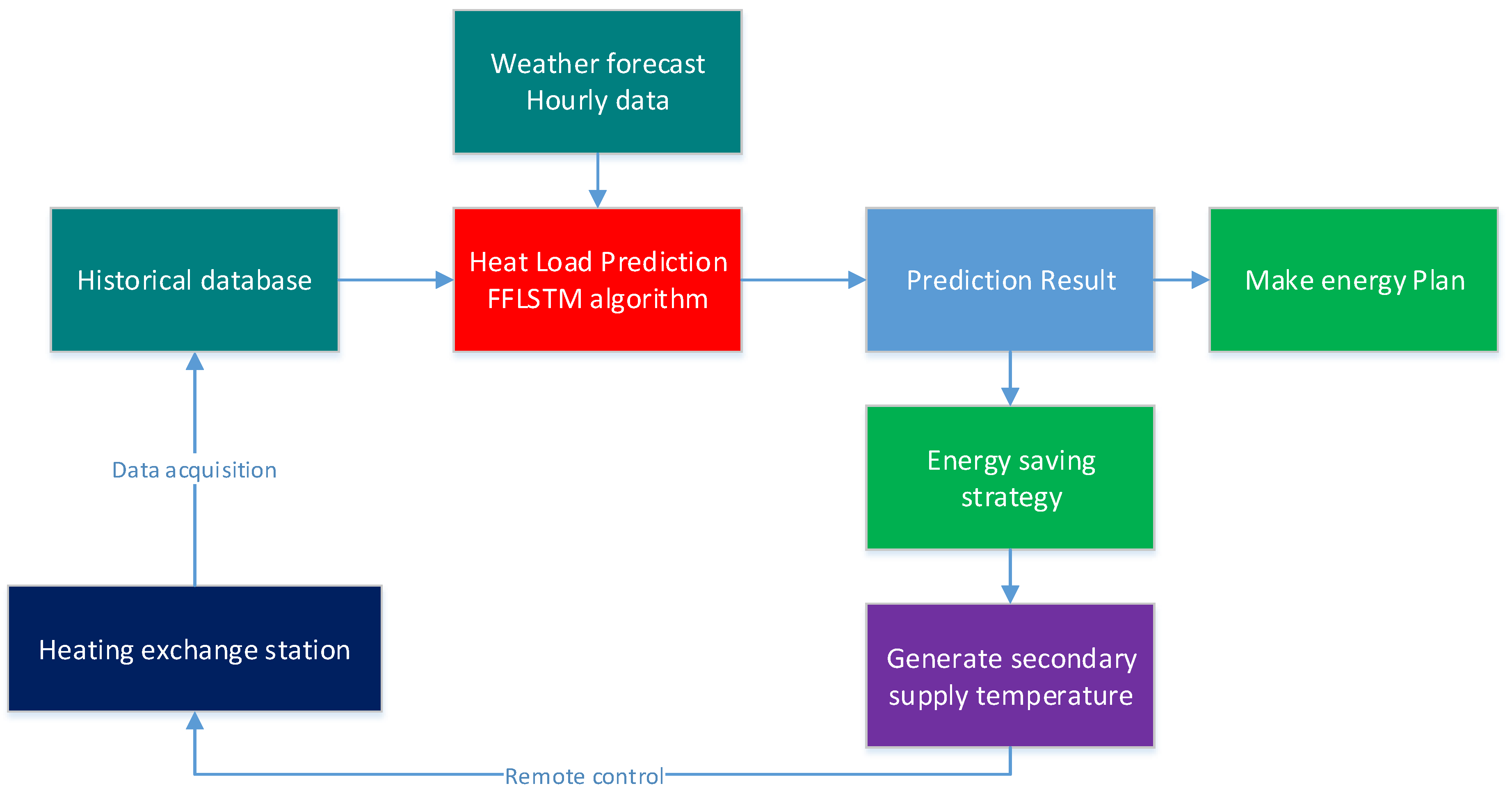
In order to further verify the prediction accuracy of the FFLSTM algorithm in the actual SDHS and its performance in formulating energy scheduling plans and improving energy efficiency, we embedded the FFLSTM algorithm into the smart district heating system of the Xingtai Heating Company for preliminary engineering verification. The operation process of the FFLSTM prediction algorithm in SDHS is shown in Figure 7.
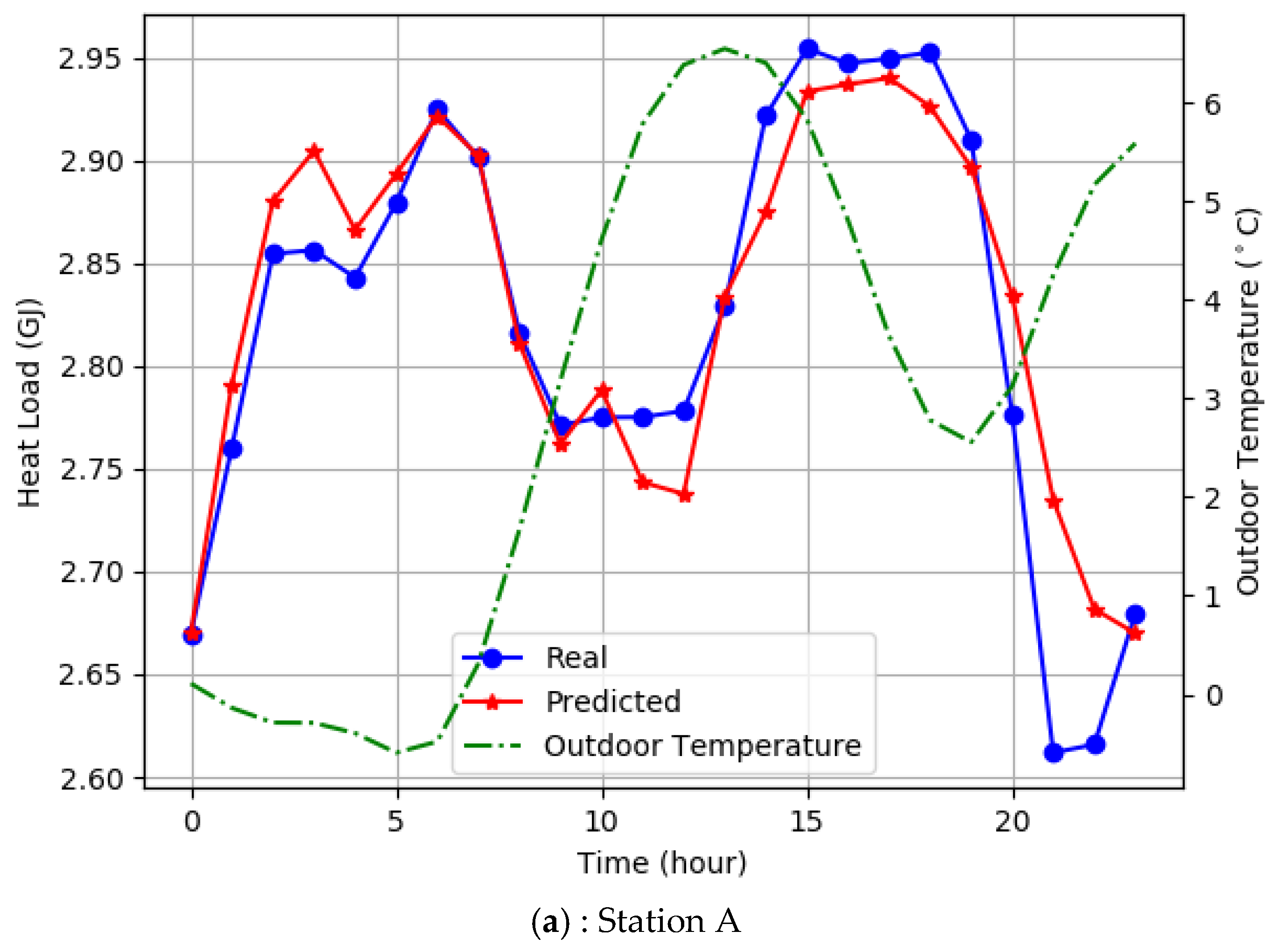
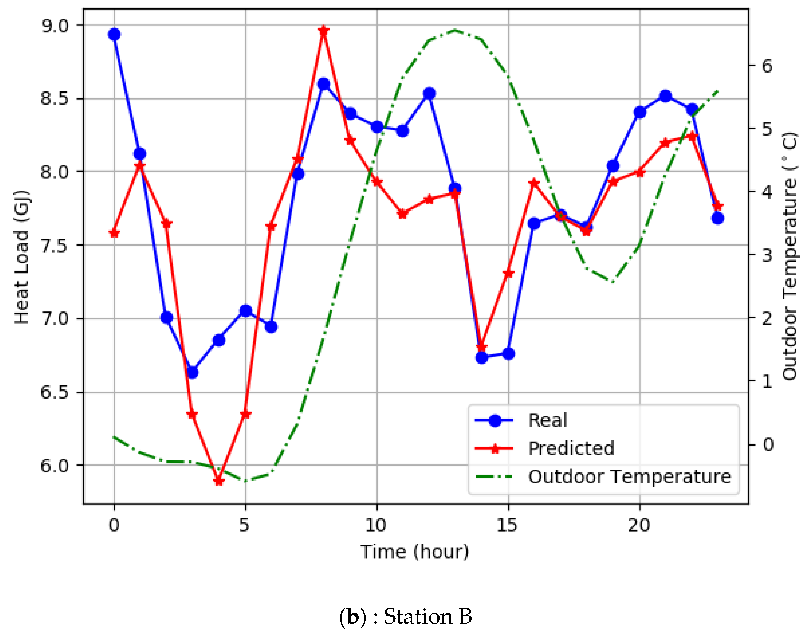
The SCADA system collects and stores the state data of the system in real time. Every night, the system regularly retrains the FFLSTM deep neural network according to the historical data collected by SCADA. With the entry of the latest proximity data, the weights of the network model will be updated and more accurate. According to the input characteristic parameters of DHS and the outdoor temperature, the FFLSTM algorithm accurately predicts the hourly heating load for the next 24 h, which is shown in Figure 8, and then the heating dispatching department formulates the next energy-saving control strategy and completes the energy production scheduling in advance.
Figure 8 shows that the FFLSTM has a high accuracy for predicting the heating load for the next 24 h, and the heating load has a significant negative correlation with the outdoor temperature—that is, the change of the heating load and outdoor temperature show a reverse trend.
In order to meet the demand adjustment of heating load caused by the rapid change of outdoor temperature, the feed forward control logic in the system responds two hours ahead of time based on the results of the heating load obtained by the FFLSTM prediction algorithm. In this way, the SDHS response speed to the outdoor temperature is accelerated, the energy-saving control effect is improved, and the indoor temperature of the user side is more stable.
Through comprehensive monitoring of the data quality, the energy consumption data of heat exchange stations are evaluated, and the energy saving and consumption reduction results are comprehensively and accurately reflected. By comparing the energy utilization before and after the system-embedded FFLSTM prediction algorithm, compared with the previous year, the heat consumption of station A and station B in 2017–2018 heating season decreased by 9.7% and 8.2%, respectively, which is shown in Table 10. The corresponding comprehensive economic cost decreased significantly.

5. Conclusions

The development of intelligent district heating systems will be a trend in the future. Accurate forecasting of the heating load based on artificial intelligence technology is the basis and guarantee of energy-saving control strategies. Such strategies can improve the energy efficiency and formulate an energy dispatching plan. The FFLSTM model for heat load prediction in a DHS was proposed in this paper. The biggest advantage of the FFLSTM algorithm is that it is a unified representation method that integrates three different time-scale characteristics—proximity, periodicity, and trend—when multiple impact factors of the heating load of the district heating system are considered. Various parameters, such as the learning rate, batch size, time step, hide unit, and iteration count, were thoroughly investigated. Detailed experimental comparisons between the proposed FFLSTM algorithm and state-of-the-art algorithms, such as LSTM, BP, SVR, RT, RFR, GBR, and ETR, were performed to verify the superiority of the proposed algorithm. It can be concluded that FFLSTM has a better prediction performance and higher accuracy compared to other prediction algorithms. Furthermore, a total of six prediction models with different time-scale features were proposed and compared in detail. Finally, we embedded the algorithm into the real SDHS and carried out preliminary engineering verification. The results show that the algorithm has a better prediction accuracy of the heating load. Combined with the feed-forward control technology, an energy-saving control strategy was constructed, which improves the energy utilization of the system. Compared with last year, the comprehensive heat consumption index was reduced by more than 8%.
In future work, we will continue to explore the optimization of an energy-saving control strategy based on artificial intelligence. In the parameter selection, the factor of indoor temperature will be added to improve the reliability and accuracy of the prediction.

Author Contributions

This paper is the fruit of all authors’ collaboration. Problem formulation and Conceptualization, G.X., T.L., Y.P., and J.S.; methodology, G.X., Y.P., and J.S.; software, Y.P. and J.S.; validation, G.X., T.L., and J.S.; data curation, G.X., T.L., and J.S.; writing—original draft preparation, G.X., T.L., Y.P., and J.S; writing—review and editing, J.S., C.Q., and Z.W.; supervision, G.X., T.L.; project administration, G.X., T.L., and J.S.

Funding

This work was supported by the National Natural Science Foundation of China (Grant No.61702157) and the Postdoctoral Fund of Hebei Province of China (No. B2017005002).

Conflicts of Interest

The authors declare no conflict of interest.

Nomenclature

ANFISadaptive neuro-fuzzy inferences system
ANNartificial neural networks
BPback propagation
DHSdistrict heating system
DLdeep learning
ELMextreme learning machines
ETRextra trees regression
FFAfirefly algorithm
FFLSTMfeature fusion long short-term memory
GAgenetic algorithm
GA–SVRgenetic algorithm–support vector regression
GBRgradient boosting regression
IAimmune algorithm
IoTInternet of Things
LSTMlong short-term memory
MAEmean absolute error
MAPEmean absolute percentage error
MVAmultivariate autoregressive
N-LSTMproximity LSTM
PLSPartial Least Square
P-LSTMperiodic LSTM
PM10particulate matter 10
PSOparticle swarm optimization
RBFradial kernel function
RFRrandom forest regression
RMSEroot-mean-square error
RNNrecurrent neural networks
RTregression tree
SCADAsupervisory control and data acquisition
SDHSsmart district heating system
SVMsupport vector machine

References

  1. Ebenstein, A.; Fan, M.Y.; Greenstone, M.; He, G.J.; Zhou, M.G. New evidence on the impact of sustained exposure to air pollution on life expectancy from China’s Huai River Policy. Proc. Natl. Acad. Sci. USA 2017, 114, 10384–10389. [Google Scholar] [CrossRef] [PubMed]
  2. Chou, J.-S.; Bui, D.-K. Modeling heating and cooling loads by artificial intelligence for energy-efficient building design. Energy Build. 2014, 82, 437–446. [Google Scholar] [CrossRef]
  3. Dotzauer, E. Simple model for prediction of loads in district-heating systems. Appl. Energy 2002, 73, 277–284. [Google Scholar] [CrossRef]
  4. Karatasou, S.; Santamouris, M.; Geros, V. Modeling and predicting building’s energy use with artificial neural networks: Methods and results. Energy Build. 2006, 38, 949–958. [Google Scholar] [CrossRef]
  5. Boithias, F.; El Mankibi, M.; Michel, P. Genetic algorithms based optimization of artificial neural network architecture for buildings’ indoor discomfort and energy consumption prediction. Build. Simul. 2012, 5, 95–106. [Google Scholar] [CrossRef]
  6. Cai, H.; Shen, S.; Lin, Q.; Li, X.; Xiao, H. Predicting the energy consumption of residential buildings for regional electricity supply-side and demand-side management. IEEE Access 2019, 7, 30386–30397. [Google Scholar] [CrossRef]
  7. Zhang, F.; Deb, C.; Lee, S.E.; Yang, J.; Shah, K.W. Time series forecasting for building energy consumption using weighted Support Vector Regression with differential evolution optimization technique. Energy Build. 2016, 126, 94–103. [Google Scholar] [CrossRef]
  8. Fan, G.-F.; Peng, L.-L.; Hong, W.-C.; Sun, F. Electric load forecasting by the SVR model with differential empirical mode decomposition and auto regression. Neurocomputing 2016, 173, 958–970. [Google Scholar] [CrossRef]
  9. Hong, W.-C. Electric load forecasting by support vector model. Appl. Math. Model. 2009, 33, 2444–2454. [Google Scholar] [CrossRef]
  10. Ding, Y.; Zhang, Q.; Yuan, T. Research on short-term and ultra-short-term cooling load prediction models for office buildings. Energy Build. 2017, 154, 254–267. [Google Scholar] [CrossRef]
  11. Wang, M.; Tian, Q. Dynamic Heat Supply Prediction Using Support Vector Regression Optimized by Particle Swarm Optimization Algorithm. Math. Probl. Eng. 2016, 2016, 3968324. [Google Scholar] [CrossRef]
  12. Al-Shammari, E.T.; Keivani, A.; Shamshirband, S.; Mostafaeipour, A.; Yee, P.L.; Petkovic, D.; Ch, S. Prediction of heat load in district heating systems by Support Vector Machine with Firefly searching algorithm. Energy 2016, 95, 266–273. [Google Scholar] [CrossRef]
  13. Lee, A.; Geem, Z.; Suh, K.-D. Determination of Optimal Initial Weights of an Artificial Neural Network by Using the Harmony Search Algorithm: Application to Breakwater Armor Stones. Appl. Sci. 2016, 6, 164. [Google Scholar] [CrossRef]
  14. Dalipi, F.; Yildirim Yayilgan, S.; Gebremedhin, A. Data-Driven Machine-Learning Model in District Heating System for Heat Load Prediction: A Comparison Study. Appl. Comput. Intell. Soft Comput. 2016, 2016, 3403150. [Google Scholar] [CrossRef]
  15. Sajjadi, S.; Shamshirband, S.; Alizamir, M.; Yee, P.L.; Mansor, Z.; Manaf, A.A.; Altameem, T.A.; Mostafaeipour, A. Extreme learning machine for prediction of heat load in district heating systems. Energy Build. 2016, 122, 222–227. [Google Scholar] [CrossRef]
  16. Roy, S.S.; Roy, R.; Balas, V.E. Estimating heating load in buildings using multivariate adaptive regression splines, extreme learning machine, a hybrid model of MARS and ELM. Renew. Sustain. Energy Rev. 2018, 82, 4256–4268. [Google Scholar]
  17. Kato, K.; Sakawa, M.; Ishimaru, K.; Ushiro, S.; Shibano, T. Heat Load Prediction through Recurrent Neural Network in District Heating and Cooling Systems. In Proceedings of the 2008 IEEE International Conference on Systems, Man And Cybernetics, Singapore, 12–15 October 2008; p. 1400. [Google Scholar]
  18. Shamshirband, S.; Petković, D.; Enayatifar, R.; Hanan Abdullah, A.; Marković, D.; Lee, M.; Ahmad, R. Heat load prediction in district heating systems with adaptive neuro-fuzzy method. Renew. Sustain. Energy Rev. 2015, 48, 760–767. [Google Scholar] [CrossRef]
  19. Qing, X.; Niu, Y. Hourly day-ahead solar irradiance prediction using weather forecasts by LSTM. Energy 2018, 148, 461–468. [Google Scholar] [CrossRef]
  20. Li, C.; Ding, Z.; Zhao, D.; Yi, J.; Zhang, G. Building Energy Consumption Prediction: An Extreme Deep Learning Approach. Energies 2017, 10, 1025. [Google Scholar] [CrossRef]
  21. Fu, G. Deep belief network based ensemble approach for cooling load forecasting of air-conditioning system. Energy 2018, 148, 269–282. [Google Scholar] [CrossRef]
  22. Liu, F.; Cai, M.; Wang, L.; Lu, Y. An ensemble model based on adaptive noise reducer and over-fitting prevention LSTM for multivariate time series forecasting. IEEE Access 2019, 7, 26102–26115. [Google Scholar] [CrossRef]
  23. Han, L.Y.; Peng, Y.X.; Li, Y.H.; Yong, B.B.; Zhou, Q.G.; Shu, L. Enhanced Deep Networks for short-Term and Medium-Term Load Forecasting. IEEE Access 2019, 7, 4045–4055. [Google Scholar] [CrossRef]
  24. Bouktif, S.; Fiaz, A.; Ouni, A.; Serhani, M.A. Optimal Deep Learning LSTM Model for Electric Load Forecasting using Feature Selection and Genetic Algorithm: Comparison with Machine Learning Approaches. Energies 2018, 11, 1626. [Google Scholar] [CrossRef]
  25. Tian, C.; Ma, J.; Zhang, C.; Zhan, P. A Deep Neural Network Model for Short-Term Load Forecast Based on Long Short-Term Memory Network and Convolutional Neural Network. Energies 2018, 11, 3493. [Google Scholar] [CrossRef]
  26. Bouktif, S.; Fiaz, A.; Ouni, A.; Serhani, M. Single and Multi-Sequence Deep Learning Models for Short and Medium Term Electric Load Forecasting. Energies 2019, 12, 149. [Google Scholar] [CrossRef]
  27. Liang, Y.; Ke, S.; Zhang, J.; Yi, X.; Zheng, Y. GeoMAN: Multi-Level Attention Networks for Geo-Sensory Time Series Prediction; IJCAI: Stockholm, Sweden, 19 July 2018; pp. 3428–3434. [Google Scholar]
  28. Lopez, E.; Valle, C.; Allende, H.; Gil, E.; Madsen, H. Wind Power Forecasting Based on Echo State Networks and Long Short-Term Memory. Energies 2018, 11, 526. [Google Scholar] [CrossRef]
  29. Shi, X.; Lei, X.; Huang, Q.; Huang, S.; Ren, K.; Hu, Y. Hourly Day-Ahead Wind Power Prediction Using the Hybrid Model of Variational Model Decomposition and Long Short-Term Memory. Energies 2018, 11, 3227. [Google Scholar] [CrossRef]
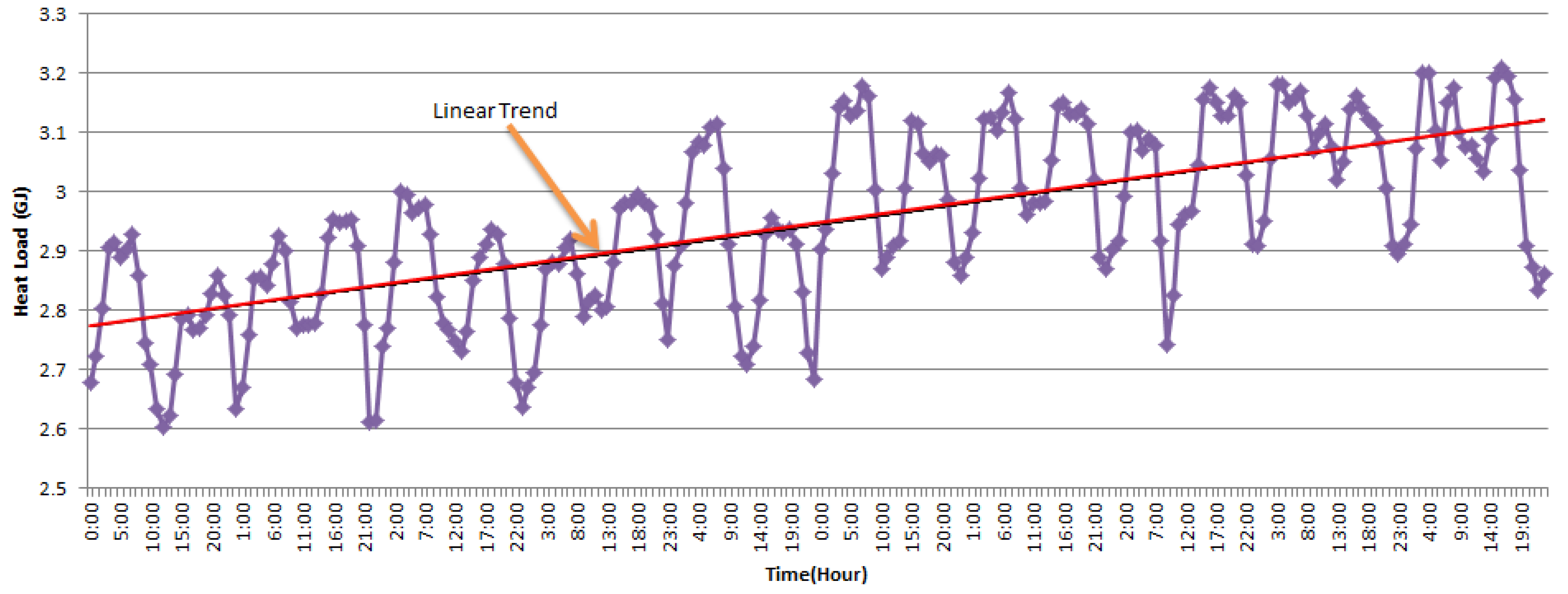
Figure 1. Time characteristics of the heat load.
Energies 12 02122 g001
Figure 2. Correlation of heat load versus each of the influencing factors. (a) Historical heat load, (b) outdoor temperature, (c) second supply temperature, (d) second return temperature, and (e) instantaneous flow rate.
Energies 12 02122 g002
Figure 3. The overall architecture of the prediction based on the fusion algorithm of time feature extraction.
Energies 12 02122 g003
Figure 4. Evaluation of the results of the root-mean-square error (RMSE) for station A and B, respectively.
Energies 12 02122 g004
Figure 5. Evaluation of the results of the mean absolute error (MAE) for station A and B, respectively.
Energies 12 02122 g005aEnergies 12 02122 g005b
Figure 6. Evaluation of the results of the mean absolute percentage error (MAPE) for station A and B, respectively.
Energies 12 02122 g006
Figure 7. The operation process of the FFLSTM prediction algorithm in a smart district heating system (SDHS).
Energies 12 02122 g007
Figure 8. The prediction result curves for the next 24 h for (a) station A and (b) station B.
Energies 12 02122 g008aEnergies 12 02122 g008b
Table 1. The input factors to heating load prediction for the related literature.
LiteratureAlgorithmInfluencing Factors
[3]ARMAoutdoor temperature, heat load, behavior of the consumers
[11]PSO–SVRoutdoor temperature, supply water temperature, supply water pressure, circular flow, heat load
[12]SVM–FFAtime lagged heat load, outdoor temperature, primary return temperatures
[14]SVR, PLS, RTforward temperature, return temperature, flow rate, heat load
[15]ELMoutdoor temperature, primary supply temperature, primary return temperature, flow on primary side
[18]ANFISoutdoor temperature, primary supply temperature, primary return temperature, secondary supply temperature, secondary return temperature, flow on primary side
Table 2. The correlation value of heat load versus other factors.
Time intervalsHistorical Heat loadOutdoor TempSupply TempReturn TempFlow Rate
p = 1 h0.913−0.3390.7670.7100.783
p = 2 h0.729−0.3010.5770.5380.549
p = 3 h0.553−0.2750.3790.3600.320
p = 4 h0.4080.2710.2060.2080.124
p = 5 h0.2910.2940.0900.1230.027
q =1 d0.765−0.2240.7680.7170.693
q = 2 d0.626−0.2190.5790.3960.524
q = 3 d0.151−0.1570.045−0.0860.140
q = 4 d−0.128−0.117−0.189−0.2830.069
r = 1 w−0.5290.257−0.545−0.5780.390
r = 2 w0.395−0.1260.7260.6910.377
* Note: h represents the hour, d represents the day and w represents the week in Table 2.
Table 3. Six models with different inputs.
ModelProximity Factor (p)Periodic Factor (q)Trend Factor (r)
model 11 h1 d1 w
model 22 h1 d1 w
model 33 h1 d1 w
model 41 h2 d1 w
model 52 h2 d1 w
model 63 h2 d1 w
Table 4. Initial parameters of the FFLSTM.
ParametersValueDescription
hide_unit20the number of hidden cells
learn_rate0.006the value of the learning rate
time_step5the value of the time step
batch_size20the value of the batch size
iter_count200the number of iterations
Table 5. The performance of heat load prediction for different selected parameters.
Parameters SetTurning ParameterValueTrainTest
RMSEMAEMAPERMSEMAEMAPE
hide_unit = 20
time_step = 5
batch_size = 20
iter_count = 200
learn_rate0.00060.0270.0200.0070.0490.0390.014
0.00010.0430.0340.0110.0530.0440.016
0.0030.0210.0140.0050.0480.0390.014
0.0010.0270.0190.0060.0480.0400.014
0.0020.0220.0140.0050.0440.0350.013
learn_rate = 0.002
hide_unit = 20
time_step = 5
iter_count = 200
batch_size50.1870.0130.0040.0450.0360.013
100.0250.0190.0060.0520.0410.015
120.0210.0150.0050.0510.0420.015
150.0220.0150.0040.0460.0380.013
200.0220.0140.0050.0440.0350.013
learn_rate = 0.002
hide_unit = 20
batch_size = 20
iter_count = 200
time_step70.0200.0130.0040.0510.0440.016
100.0210.0160.0050.0510.0420.015
120.0210.0150.0050.0380.0290.011
150.0190.0130.0040.0540.0420.015
200.0190.0140.0050.0450.0370.013
learn_rate = 0.002
batch_size = 20
time_step = 12
iter_count = 200
hide_unit50.0330.0250.0090.0310.0260.009
70.0290.0230.0080.0410.0340.012
100.0230.0170.0060.0350.0310.011
120.0220.0170.0060.0460.0340.012
150.0190.0140.0050.0440.0350.013
Note: The text in red bold font is the optimal prediction result of the given algorithm for each model.
Table 6. Final parameter selection.
ParametersValueDescription
hide_unit5the number of hidden cells
learn_rate0.002the value of the learning rate
time_step12the value of the time step
batch_size20the value of the batch size
iter_count200the number of iterations with early stopping
Table 7. The FFLSTM compared with the base short-term memory (LSTM) model.
AlgorithmModelStation AStation B
RMSEMAEMAPERMSEMAEMAPE
FFLSTMmodel 10.0430.0350.0120.6240.4910.064
N-LSTM0.0500.0390.0140.7070.5750.074
P-LSTM0.0990.0870.0311.2050.9530.128
T-LSTM0.1290.1130.0401.0610.8830.118
FFLSTMmodel 20.0440.0400.0140.5180.4140.055
N-LSTM0.0450.0340.0120.6940.5930.079
P-LSTM0.1040.0890.0311.4681.0860.149
T-LSTM0.1310.1070.0381.0380.8820.117
FFLSTMmodel 30.0390.0280.0100.5890.4530.060
N-LSTM0.0390.0290.0100.9200.6990.093
P-LSTM0.1060.0950.0331.3250.9550.128
T-LSTM0.1360.1050.0371.2231.0100.131
FFLSTMmodel 40.0480.0350.0120.5120.4220.056
N-LSTM0.0480.0350.0130.8340.5970.081
P-LSTM0.0720.0630.0221.4481.1290.153
T-LSTM0.0970.0810.0291.5111.1300.157
FFLSTMmodel 50.0650.0500.0180.4280.3350.044
N-LSTM0.0660.0550.0200.7630.6140.084
P-LSTM0.0880.0760.0270.9640.7600.102
T-LSTM0.1330.1010.0350.9990.7980.109
FFLSTMmodel 60.0420.0320.0120.4850.3810.049
N-LSTM0.0450.0350.0130.6990.5790.078
P-LSTM0.0900.0740.0261.0710.8780.115
T-LSTM0.0970.0780.0281.2321.0140.136
Note: The text in red bold font is the optimal prediction result of the given algorithm for each model.
Table 8. The performance comparison of different algorithm for six models.
AlgorithmModelStation AStation B
RMSEMAEMAPERMSEMAEMAPE
FFLSTMmodel10.0430.0350.0120.7070.5750.074
LSTM0.0700.0560.0201.1090.8500.112
BP0.0770.0650.0230.7500.5490.073
SVR(RBF)0.1240.1000.0361.1210.9300.122
RT0.1330.1060.0381.2160.9940.131
RFR0.1330.1070.0381.1720.9570.126
GBR0.1270.1030.0371.2010.9800.128
ETR0.1390.1110.0401.1550.9470.124
FFLSTMmodel20.0440.0400.0140.5180.4140.055
LSTM0.0710.0560.0200.7660.5900.077
BP0.0600.0470.0171.1910.9660.137
SVR(RBF)0.1230.1000.0361.1090.9210.122
RT0.1400.1100.0391.2821.0420.140
RFR0.1370.1110.0401.2100.9830.128
GBR0.1330.1070.0391.1760.9600.126
ETR0.1330.1080.0391.1570.9480.124
FFLSTMmodel30.0390.0280.0100.5890.4530.060
LSTM0.0500.0420.0151.2791.0410.141
BP0.0580.0460.0161.1910.9660.137
SVR(RBF)0.1220.1220.0361.0960.9120.121
RT0.1440.1140.0411.3931.1430.150
RFR0.1310.1050.0381.1700.9640.127
GBR0.1320.1070.0381.1730.9600.127
ETR0.1320.1070.0381.1890.9720.127
FFLSTMmodel40.0330.0270.0100.5560.4450.058
LSTM0.0900.0680.0251.0590.8320.108
BP0.0660.0500.0181.1910.9660.137
SVR(RBF)0.1230.1000.0361.1100.9230.120
RT0.1330.1060.0381.2341.0060.132
RFR0.1220.0980.0351.2100.9820.128
GBR0.1420.1160.0411.1740.9630.125
ETR0.1300.1060.0381.1670.9620.126
FFLSTMmodel50.0550.0370.0130.5720.4140.056
LSTM0.1050.0750.0271.1690.9690.129
BP0.0680.0510.0181.1910.9660.137
SVR(RBF)0.1220.0990.0361.0930.9130.119
RT0.1360.1070.0391.2831.0510.139
RFR0.1310.1050.0381.1690.9620.126
GBR0.1410.1150.0411.1490.9440.123
ETR0.1290.1040.0381.1060.9180.119
FFLSTMmodel60.0300.0260.0090.5350.4040.055
LSTM0.0680.0540.0191.5401.1930.166
BP0.0660.0520.0191.1910.9660.137
SVR(RBF)0.1220.0980.0351.0860.9090.119
RT0.1340.1060.0381.4671.1620.154
RFR0.1280.1030.0371.1730.9610.127
GBR0.1400.1140.0411.1500.9440.124
ETR0.1250.1010.0361.1230.9330.122
Note: The text in red bold font is the optimal prediction result of given algorithm for each model.
Table 9. The accuracy for the final prediction model.
AlgorithmStation AStation B
Accuracy (%)Accuracy (%)
FFLSTM98.8794.03
LSTM97.987.78
BP98.1587.37
SVR(RBF)96.4287.95
RT96.1285.9
RFR96.8787.3
GBR96.0587.45
ETR96.1887.63
Note: The text in red bold font is the optimal prediction result of the given algorithm for each model.
Table 10. The comparison of the energy utilization for station A and station B.
YearHeat Consumption (GJ)
Station A Station B
201710,76231,601
2018971129,010
Energy saving rate9.7%8.2%