New Perspective on Performances and Limits of Solar Fresh Air Cooling in Different Climatic Conditions

Abstract

The study carried out by simulation, concerns the thermal behavior of an office building’s solar fresh air cooling system, based on a LiBr-H₂O absorption chiller in different climatic conditions. The coefficient of performance (COP) and the solar fraction were considered performance parameters and were analyzed with respect to the operating limits—the risk of crystallization and maintaining at least a minimum degassing zone. A new correlation between the required solar hot temperature and the cooling water temperature was established and then embedded in another new correlation between the COP and the cooling water temperature that was used in simulations during the whole cooling season corresponding to each location. It was found that—the solar hot water should be maintained in the range of (80–100) °C depending on the cooling water temperature, the COP of the solar LiBr-H₂O absorption chiller with or without cold storage tank could reach (76.5–82.4)% depending on the location, and the solar fraction could reach (29.5–62.0)% without cold storage tank and could exceed 100% with cold storage tank, and the excess cooling power being available to cover other types of cooling loads—through the building envelope, from lighting, and from occupants, etc.

1. Introduction

The building sector accounts for 40% of the global energy consumption [1] and heating ventilation and air conditioning (HVAC) is one of the major energy consumers in buildings [2]. Additionally, global warming is expected to cause more overheating in buildings [3].

Since solar radiation is a major component of the cooling load, there is also a challenge to convert solar radiation into useful forms of energy [4]. Solar radiation directly influences the cooling load of buildings, thus the two are correlated at least to a certain extent [5].

Under these circumstances, solar cooling systems and particularly solar fresh air cooling systems (SFACS) have been a major research topic in the last few years. Between several other solar cooling technologies, the solar absorption cooling systems (SACS) were found to be the most energy efficient for six major cities in Australia [6]. SACS are considered a sustainable solution for solar driven air conditioning equipment, particularly in warmer climates, even though some problems related to these systems still exist [7,8]. Based on the coefficient of performance (COP), SACS are more efficient than other systems, such as the adsorption ones [9].

Between several working agents, the LiBr-H₂O solution is considered one of the most preferable options because it can provide the best annual performance [9], it is ecofriendly because water is used as the refrigerant, and it provides an excellent cooling potential due to the high latent heat of water [10].

The most widespread version of LiBr-H₂O SACS is the single effect one and several studies have been dedicated to this type of equipment by experiment [4,11] or by modelling [12,13].

Even though air cooling is considered in several studies, all the LiBr-H₂O absorption chillers that are currently on the market are water-cooled [14] and only a single model of an air-cooled single effect LiBr-H₂O absorption chiller has ever been marketed and was only available from 2005 to 2008 [14].

One of the main reasons why the expansion of air cooled LiBr-H₂O was limited is the crystallization risk under ambient conditions [15]. This problem also occurs with water-cooled LiBr-H₂O absorption systems, because LiBr is a salt with a crystalline structure and will crystallize at any concentration below a certain temperature [16]. This concern is a major operating issue of these systems. The possibility of avoiding the crystallization problem was investigated in some studies including [8,17]. Despite these concerns, recommendations related to the accepted operating conditions capable of avoiding crystallization in solar LiBr-H₂O SACS are not easily available in literature.

Another operating problem of SACS is providing a minimum concentrations difference between the diluted and the concentrated solution, named the degassing zone. This parameter is important because the solutions flow rates depend on the degassing zone, and low values of degassing zone determines high solutions flow rates [7,10,13]. Despite the dependence between the degassing zone and the solutions flow rates for the LiBr-H₂O, recommendations for the minimum acceptable degassing zone are not available in literature.

The SACS can be driven by hot water with a relatively low temperature that can be provided by the common flat or evacuated tubes solar thermal collectors [6,9]. Concentrating solar collectors are also used in some solar cooling studies [5,13].

In order to provide more constant cooling power, several SACS are equipped with hot water storage tanks, but in some cases, cold water storage is preferred because of lower losses [4].

The goal of this study is to provide both the performances and limits of water cooled LiBr-H₂O SACS in different operating conditions. The COP of the absorption system and the solar fraction were evaluated as the efficiency parameters. A new correlation between the required solar hot temperature and the cooling water temperature was established and then embedded in the new correlation between the COP and the cooling water temperature. This correlation was used in simulations during the whole cooling season corresponding to each location. The risk of crystallization and the minimum degassing zone were considered the limitations from an operating conditions’ point of view. The study continues from previous investigations related to the energy efficiency in buildings—the use of phase change materials in fresh air cooling systems [18]; evaluation of performances and limits of solar driven absorption chillers [17]; presentation of long term experimental study of a geothermal heat pump [19]; or evaluation of indirect evaporative cooling performances [20].

2. Materials and Methods

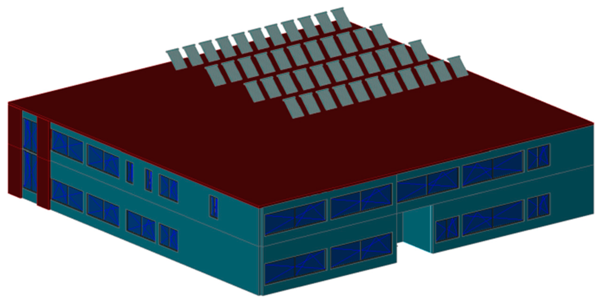
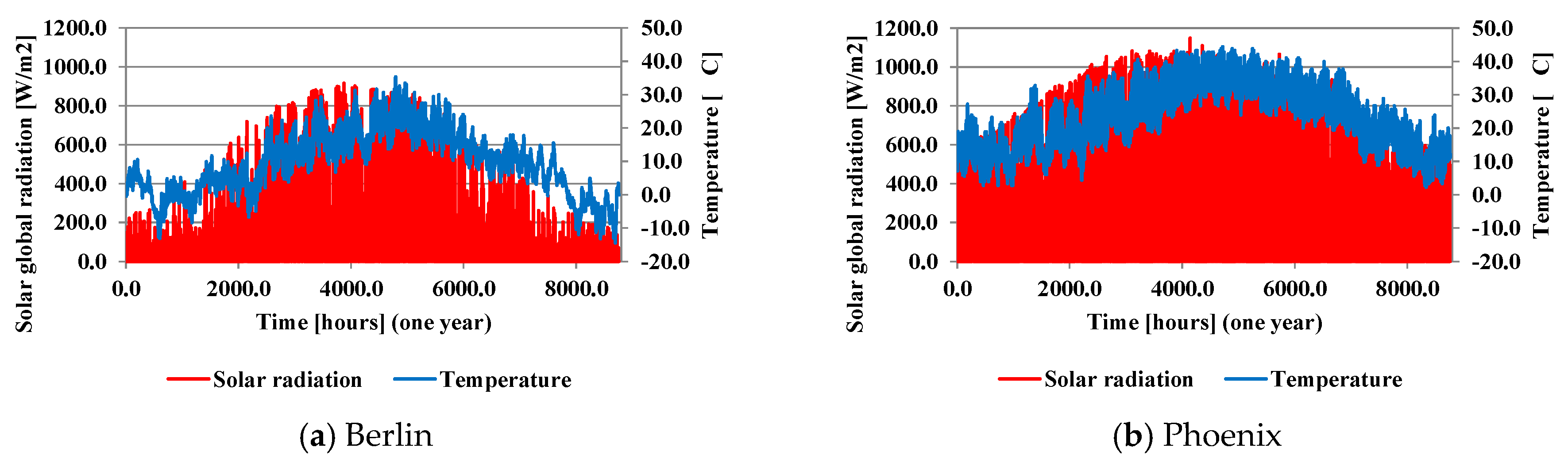
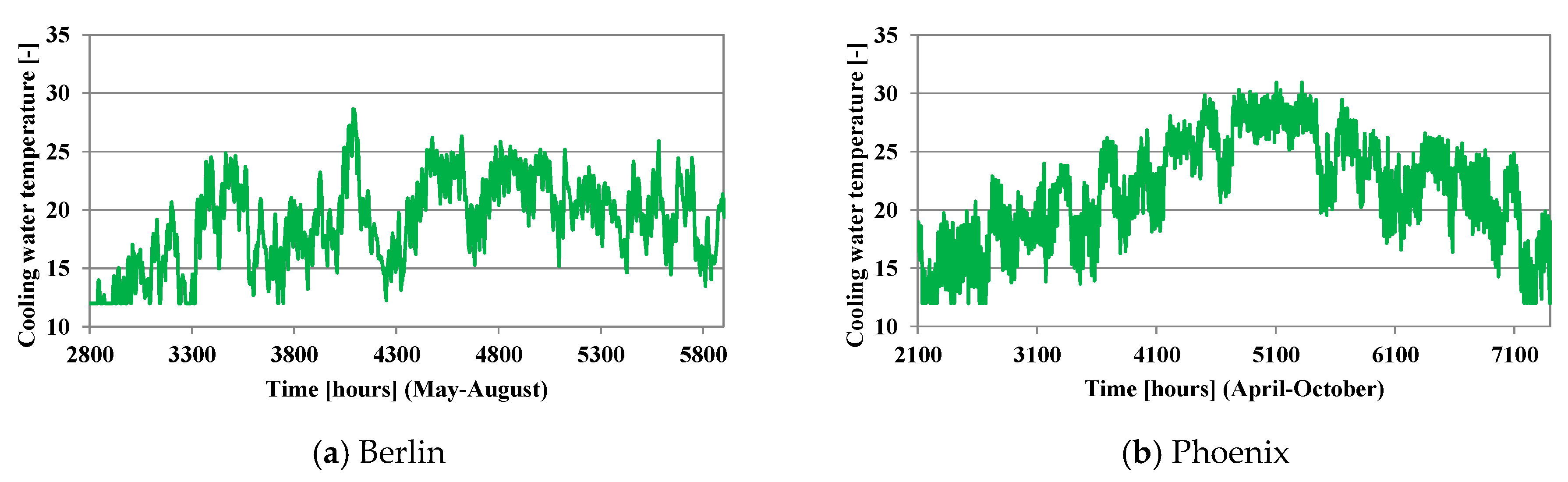
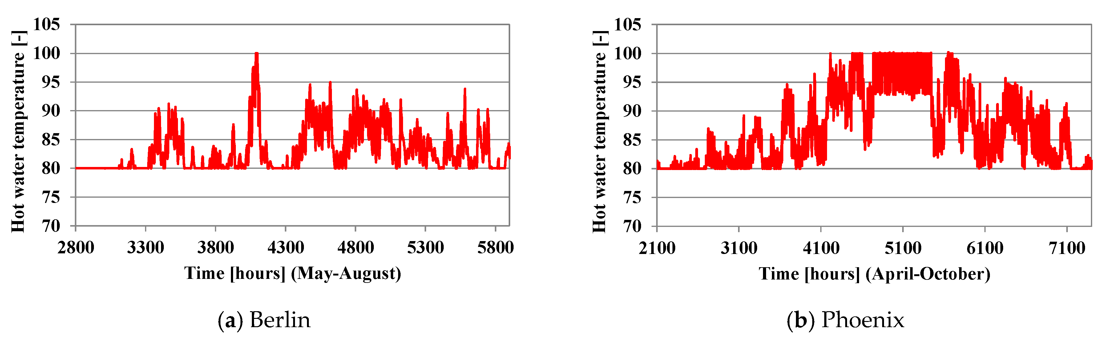
2.1. Characteristics of the Building and Climatic Conditions

The office building that was completely characterized and previously investigated in [18] was also considered in this study, situated in different locations worldwide to evaluate the influence of climatic conditions on the solar cooling system.

A 3D drawing of the building with solar thermal collectors placed on the roof is presented in Figure 1.

The solar thermal collectors are oriented to the South.

The climatic characteristics of the locations considered in this study, according to the Köppen-Geiger classification, are presented in

Table 1. Climatic characteristics of the locations.

Location	Country	Latitude (°)	Longitude (°)	Altitude (m)	Time Zone (hours)	Climate Classification	Climate Description
Berlin	DEU	52.517 N	13.389 E	44	1	Dfb	Warm humid continental climate
Paris	FRA	48.857 N	2.351 E	30	1	Cfb	Oceanic climate
Monaco	FRA	43.731 N	7.420 E	2	1	Csa	Hot-summer Mediterranean climate
Rome	ITA	41.893 N	12.483 E	42	1	Csa	Hot-summer Mediterranean climate
Seville	ESP	37.094 N	2.358 E	499	1	Csa	Hot-summer Mediterranean climate
Cairo	EGY	30.049 N	31.244 E	41	2	BWh	Hot desert climate
Phoenix	USA	33.450 N	111.983 W	337	−7	BWh	Hot desert climate
Las Vegas	USA	30.083 N	115.15 W	648	−8	BWk	Tropical and subtropical desert climate

.

The climatic data for each location was based on the available typical meteorological year (TMY). The use of the TMY data is typical for several studies related to the energy efficiency in buildings like [21,22]. The TMY presents hourly based variations of several climatic parameters like—the global solar radiation on the horizontal plane (I (W/m²)), the ambient (or dry bulb) temperature (t_db (°C)), the direct (I_dir (W/m²)) and diffuse (I_dif (W/m²)) solar radiation on the horizontal plane, the relative humidity of air (φ (%)), and the wet bulb temperature (t_wb (°C)) etc.

The variations of the input data and of the calculated values of different parameters were presented for only two representative locations corresponding to the minimum and maximum values of different TMY based criteria as presented in

Table 2. Locations with minimum and maximum values of climatic parameters.

TMY Based Criteria	Min	Max
Total yearly global solar radiation on horizontal plane	Berlin	Cairo
Maximum dry bulb temperature	Monaco	Las Vegas, Phoenix
Maximum wet bulb temperature	Berlin	Phoenix

.

Since there were five locations that reached at least one minimum or maximum value for one of the three climatic criteria (Berlin, Monaco, Cairo, Las Vegas, and Phoenix), Berlin was selected with two minimum values and Phoenix was selected with two maximum values. All of the data variations were represented only for the two selected locations.

The yearly variation of the global solar radiation on the horizontal plane and of ambient temperature for the locations of Berlin and Phoenix are presented in Figure 2.

The following data relevant to the HVAC studies, corresponding to each location, are presented in

Table 3. TMY based data characteristics for each location.

Location	Total Yearly Global Solar Radiation on Horizontal Plane (kWh/m2/year)	Maximum Dry Bulb Temperature (°C)	Maximum Wet Bulb Temperature (°C)
Berlin	1077	35.4	23.6
Paris	1153	32.5	23.8
Monaco	1595	28.1	25.2
Rome	1669	32.1	24.8
Seville	1851	40.4	25.2
Cairo	2209	39.7	24.7
Phoenix	2094	44.4	26.0
Las Vegas	2032	44.4	24.4

—the total yearly global solar radiation on the horizontal plane, the maximum ambient temperature, and the maximum wet bulb temperature.

Solar radiation is important because it is the driving parameter for both the cooling load of the building and the solar cooling system. The dry bulb temperature is important because it represents the inlet air temperature in the HVAC system. The wet bulb temperature is also important because it influences the cooling water temperature at the outlet of the cooling towers. Important differences can be observed between all of the presented parameters.

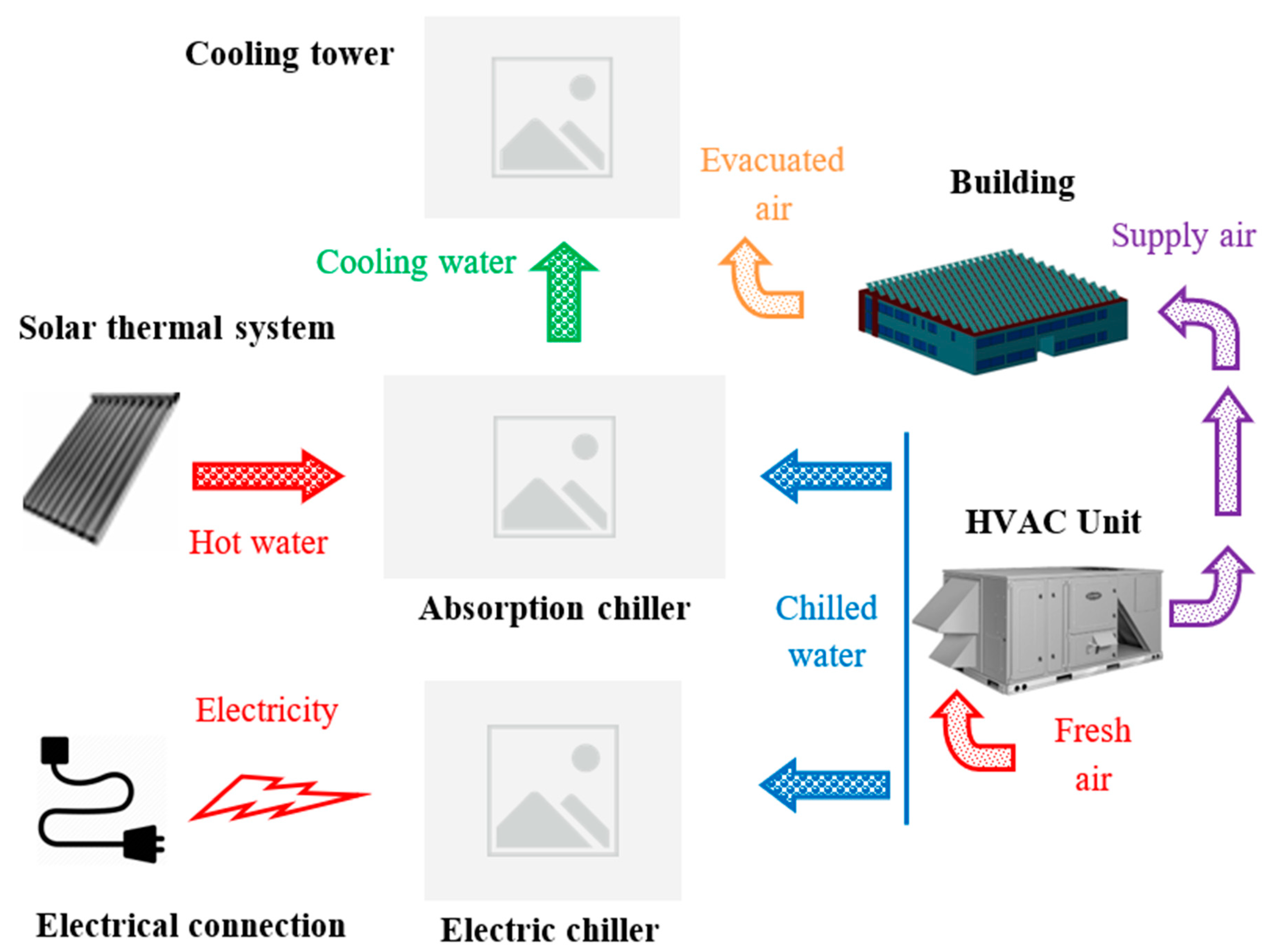
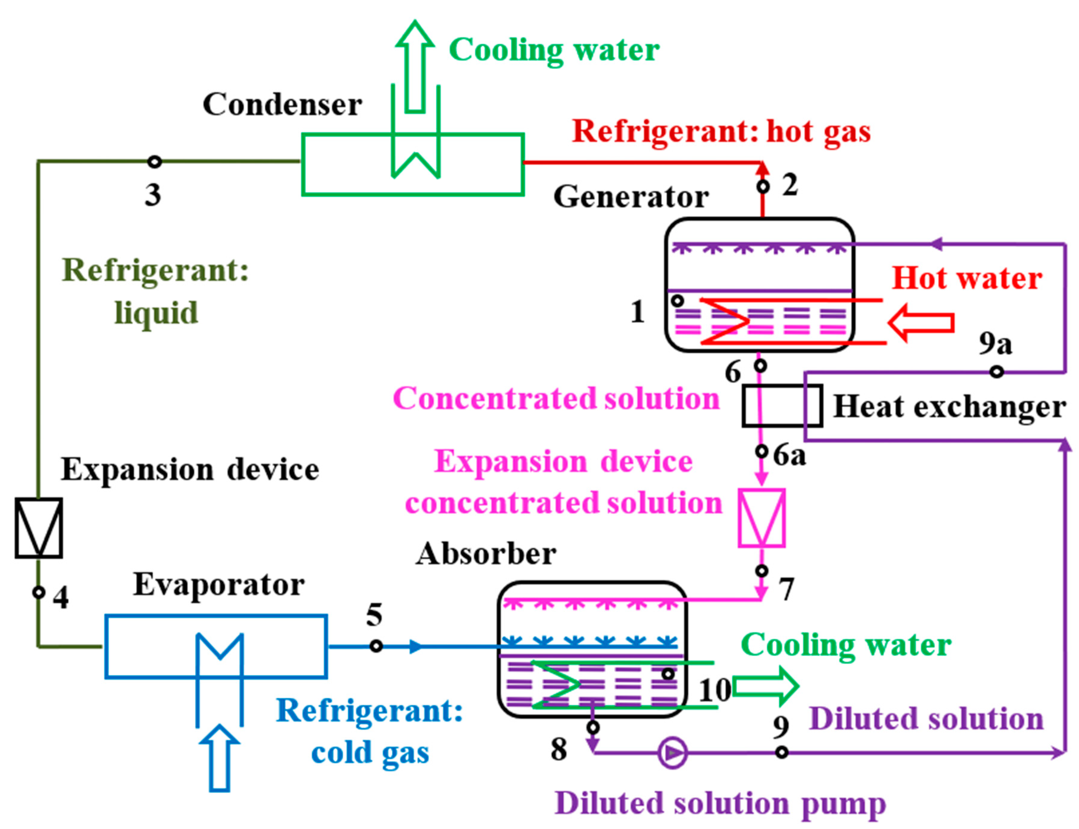
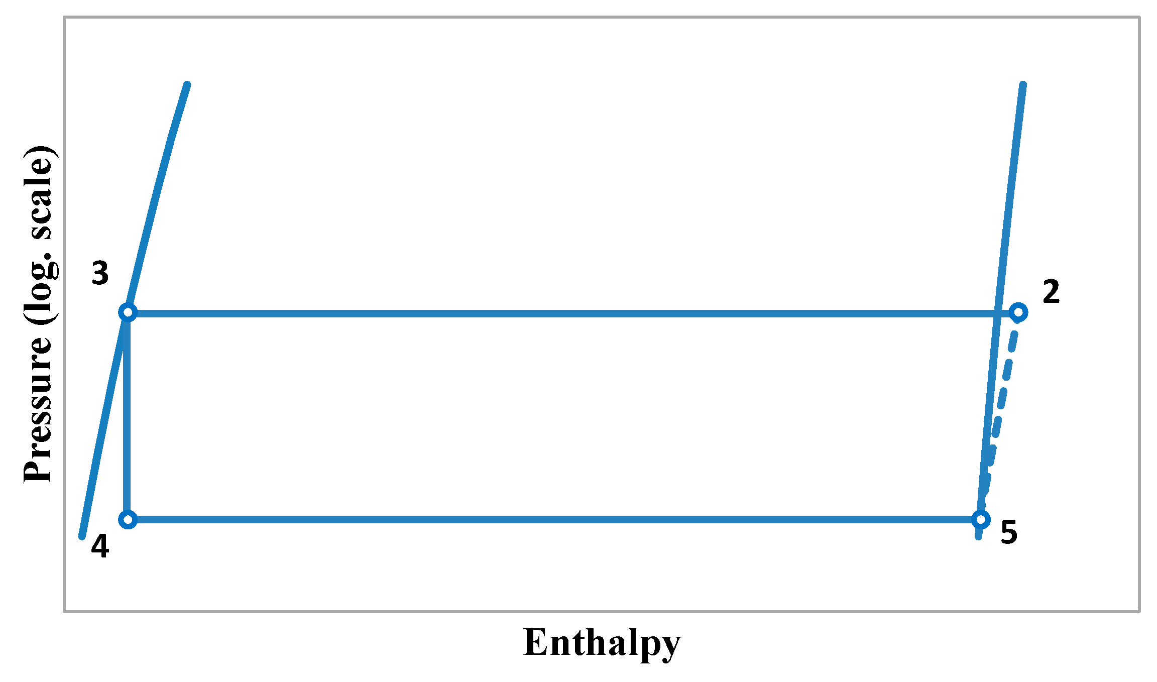
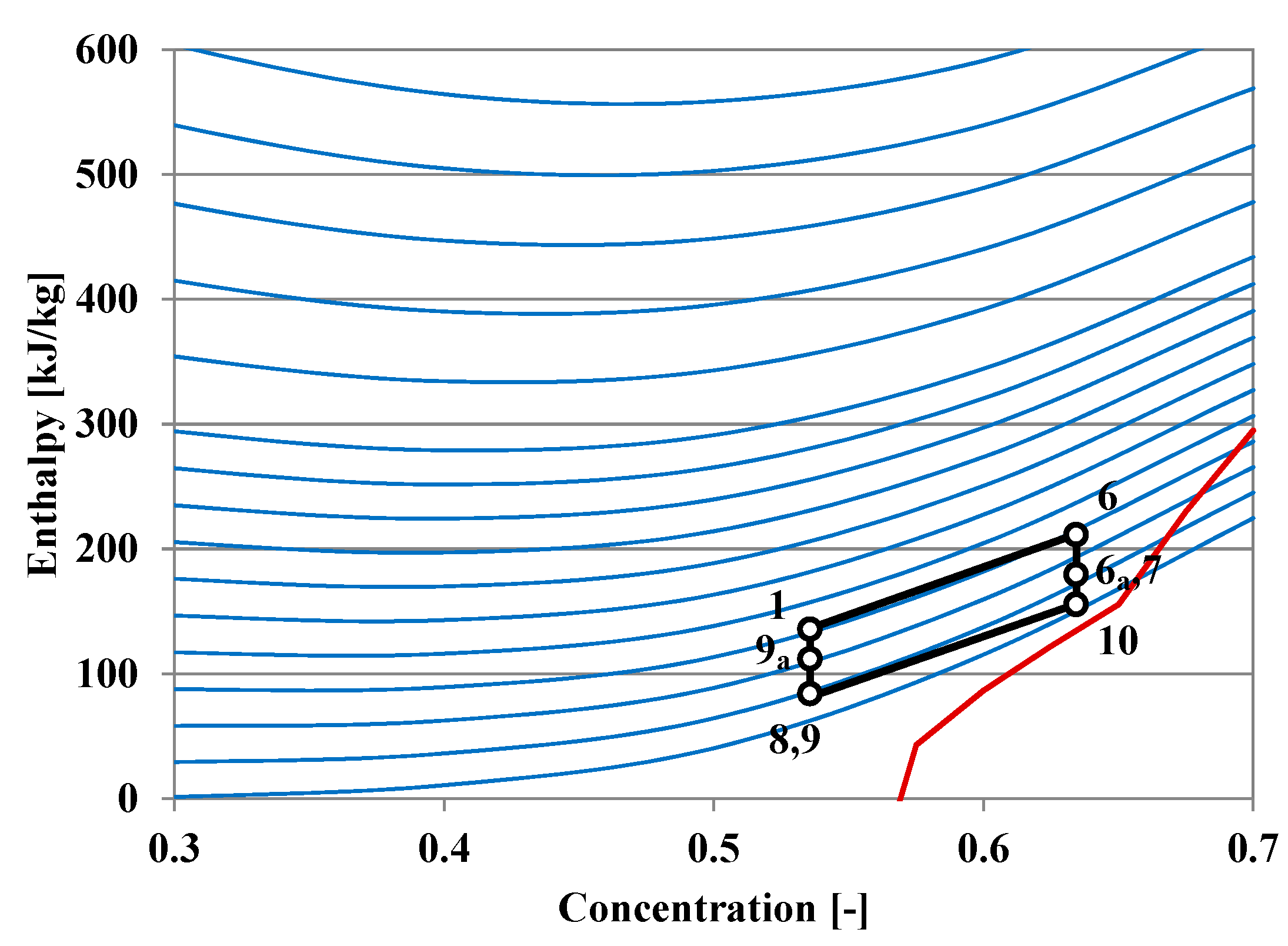
2.2. Characteristics of the Solar Cooling System

The considered fresh air solar cooling system was of the LiBr-H₂O absorption type and is presented as an energy flow scheme in Figure 3.

The fresh air cooling system included a HVAC unit, where the fresh air was cooled in a fan and the coil heat exchanger which was supplied with cold water from a LiBr-H₂O absorption chiller driven by the hot water provided by the solar thermal system. The effect of a cold water storage tank on the characteristics of the solar cooling system was also evaluated.

The cooling of the absorption chiller was provided by a cooling water circuit, equipped with an adequate water cooling tower.

If the cooling power of the solar driven absorption chiller was not sufficient, the auxiliary electric chiller starts running to complete the required cooling power.

In this study, the electrical energy required for recirculating the chilled water, the hot water, and the cooling water were neglected, being much lower than the electrical energy required to run the compressor of the electric chiller.

The principle scheme of the LiBr-H₂O solar absorption chiller is presented in Figure 4.

The main refrigerating circuit was composed of the condenser, the expansion device, and the evaporator, while the thermochemical compressor was composed of the following components—the absorber; the diluted solution pump; the generator; the expansion device of the concentrated solution; and the heat exchanger. The refrigerant of the absorption chiller was H₂O, while LiBr was the solvent. The working process of the main refrigerating circuit is presented in Figure 5 in the pressure-enthalpy diagram, while the working process of the LiBr-H₂O solution is presented in Figure 6 in the enthalpy-concentration diagram.

The red line on the enthalpy-concentration diagram represents the crystallization curve and the working states of the LiBr-H₂O solution must always be above this curve. Crystallization was avoided if the temperature in the closest state (t₁₀ (°C)) was higher than the crystallization temperature (t_cr (°C)):

$$t_{10}>t_{cr}$$

(1)

The difference between the concentrations of the diluted solution (ζ_d (%)) and the concentrated solution (ζ_c (%)), representing the degassing zone (Δζ = ζ_d − ζ_c (%)), must be maintained higher than a minimum value (Δζ_min (%)). In this study Δζ_min = 6%.

The standard thermal regime of the chilled water circuit was identical for both the absorption chiller and electric chiller and was characterized by the flow temperature (t_f = 7 °C) and return temperature (t_r = 12 °C). If, due to the operating conditions of the absorption chiller, this thermal regime could not be reached, an alternative chilled water thermal regime of 12–17 °C was used.

The thermal regime of the cooling water circuit depended on the ambient air temperature and humidity. The flow temperature on the cooling water circuit (t_fc (°C)) was dependent on the wet bulb temperature. The return temperature on the cooling water circuit (t_rc (°C)) was controlled to maintain a constant temperature difference (Δt_wc = t_rc − t_fc = 5 °C).

The thermal regime of the solar hot water was determined by the flow temperature (t_fh (°C)) and return temperature (t_rh (°C)) of the hot water. The flow rate of the hot water circuit was controlled to maintain a temperature difference (Δt_h = t_fh − t_rh = 5 °C). The hot water parameters must avoid crystallization and must ensure at least the minimum value of the degassing zone.

The internal working conditions were determined as a function of the external working conditions.

The evaporating temperature (t₀ (°C)) was determined as a function of the return temperature on the chilled water circuit:

$$t_0=t_r-\Delta t_0$$

(2)

where Δt₀ = 8 °C.

The condensing temperature (t_k (°C)) was determined as a function of the flow temperature on the cooling water circuit:

$$t_k=t_{fc}-\Delta t_k$$

(3)

where Δt_k = 8 °C.

The diluted solution temperature at the outlet of the absorber (t₈ (°C)) was considered equal to the condensing temperature and the temperature at the outlet of the generator (t₆ (°C)) was considered lower than the flow temperature of the hot water circuit:

$$t_6=t_{fh}-\Delta t_g$$

(4)

where Δt_g = 10 °C.

The sub-cooling of the diluted solution at the outlet of the heat exchanger was considered (Δt_s = t₆ − t_6a = 10 °C).

The state parameters of the water and the LiBr-H₂O solutions (including enthalpy, temperature, pressure, concentration, etc.) together with the thermal power of all of the absorption chiller components were determined using the Engineering Equation Solver (EES) software platform of F-Chart Software, Madison USA.

The mass flow rate on the main refrigerating ($\dot{m}$ (kg/s)) circuit was determined as:

$$\dot{m}=\frac{\dot{Q}}{\left(h_5-h_4\right)}$$

(5)

The mass flow rates of the diluted solution (${\dot{m}}_d$ (kg/s)) and the concentrated solution (${\dot{m}}_c$ (kg/s)) were determined from the mass balance and water balance of the absorber:

$${\dot{m}}_d=\dot{m}\frac{\left(1-x_8\right)}{\left(x_8-x_7\right)};{\dot{m}}_c=\dot{m}-{\dot{m}}_d$$

(6)

The enthalpy of the diluted solution at the heat exchanger outlet was determined as:

$$h_{9a}=\frac{\left({\dot{m}}_c·\left(h_6-h_{6a}\right)+{\dot{m}}_d·h_9\right)}{{\dot{m}}_d}$$

(7)

The thermal power of the condenser (${\dot{Q}}_k$ (kW)) was determined as:

$${\dot{Q}}_k=\dot{m}·\left(h_2-h_3\right)$$

(8)

The thermal power of the absorber (${\dot{Q}}_{Ab}$ (kW)) was determined as:

$${\dot{Q}}_{Ab}=\dot{m}·h_5+{\dot{m}}_c·h_7-{\dot{m}}_d·h_8$$

(9)

The thermal power of the generator (${\dot{Q}}_G$ (kW)) was determined as:

$${\dot{Q}}_G=\dot{m}·h_2+{\dot{m}}_c·h_6-{\dot{m}}_d·h_{9a}$$

(10)

The coefficient of performance (COP (-)) was determined as:

$$COP=\frac{{\dot{Q}}_0}{{\dot{Q}}_G}$$

(11)

The mathematical algorithm was implemented in the Engineering Equation Software (EES) that solves coupled non-linear algebraic and differential equations. An important feature of this software platform is the capability to calculate the thermodynamic and transport properties for numerous substances. The mathematical model of the LiBr-H₂O absorption chiller was already used and validated in [17]. All the other calculations were implemented in Excel and were carried out on an hourly basis due to the hourly input data of the TMY.

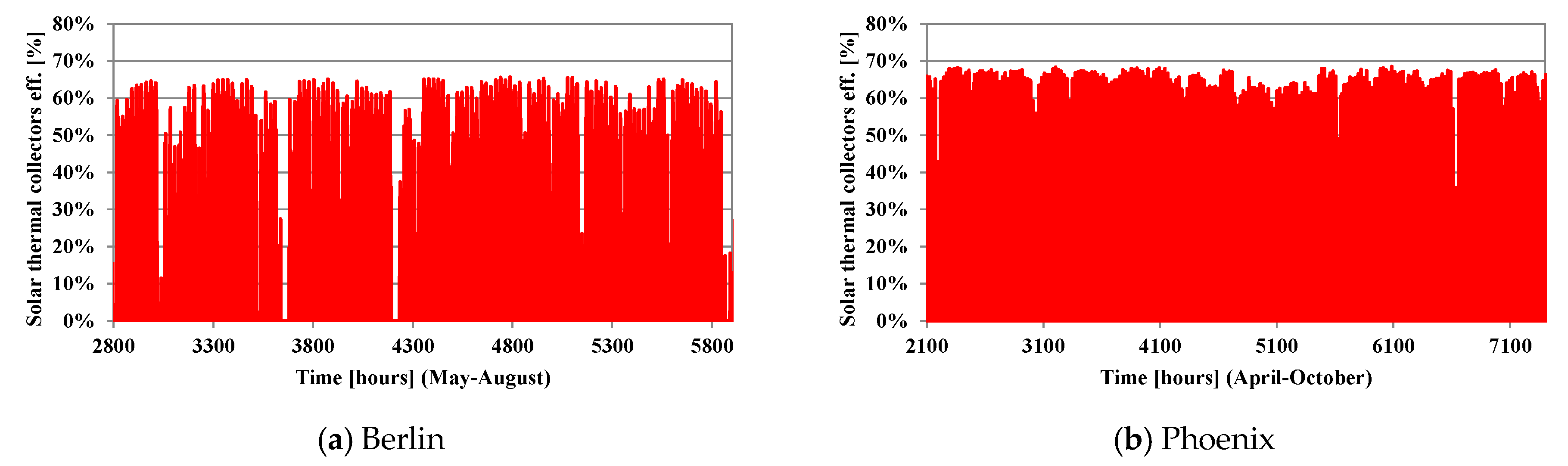
2.3. Characteristics of the Solar Thermal Collectors

The hot water that drives the absorption chiller was provided by a solar thermal system. In this study evacuated tubes solar collectors (ETSC) of SolarUK LaZer2 type were considered.

The efficiency of the ETSC (η_th (-)) was determined as [23,24,25]:

$${\eta }_{th}={\eta }_0-a_1\frac{t_{avg}-t_a}{I_{gt}}-a_2\frac{{\left(t_{avg}-t_a\right)}^2}{I_{gt}}$$

(12)

where η₀ = 0.753 is the optical efficiency of the collector, while a₁ = 1.54 W/m²K and a₂ = 0.0099 W/m²K² are coefficients of heat loss. The aperture area of this collector is of 1.864 m². These values of the ETSC parameters are public, in the test report factsheet of the considered collector, provided by the SPF Institute for Solar Technology.

t_avg (°C) is the average temperature of the hot water in the collectors, t_a (°C) is the ambient air temperature, and I_gt (W/m²) is the incident solar radiation on the tilted plane of the ETSC.

In this study, the temperature variation of the hot water in the ETSC was considered to be 20 °C and the outlet solar hot water temperature was considered dependent on the absorption chiller cooling water temperature.

Figure 7 presents the ETSC thermal efficiency for the two locations.

These values were in good agreement with the literature—65% [15], 60–75% [26], 78% [4], 73% [27], and 45–70% [28].

3. Results and Discussion

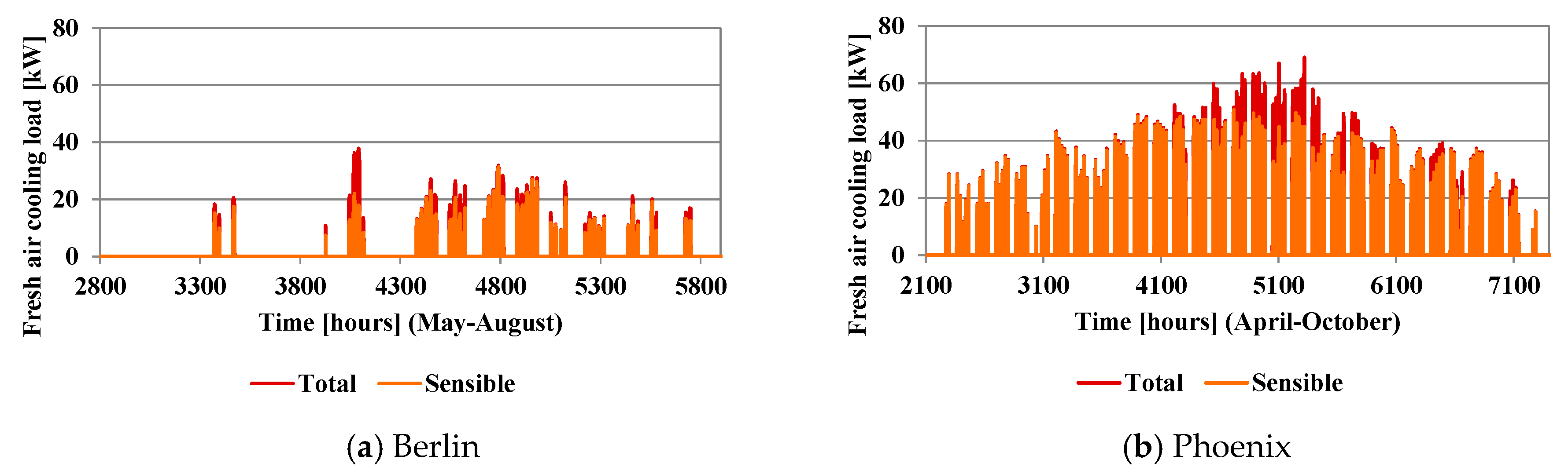
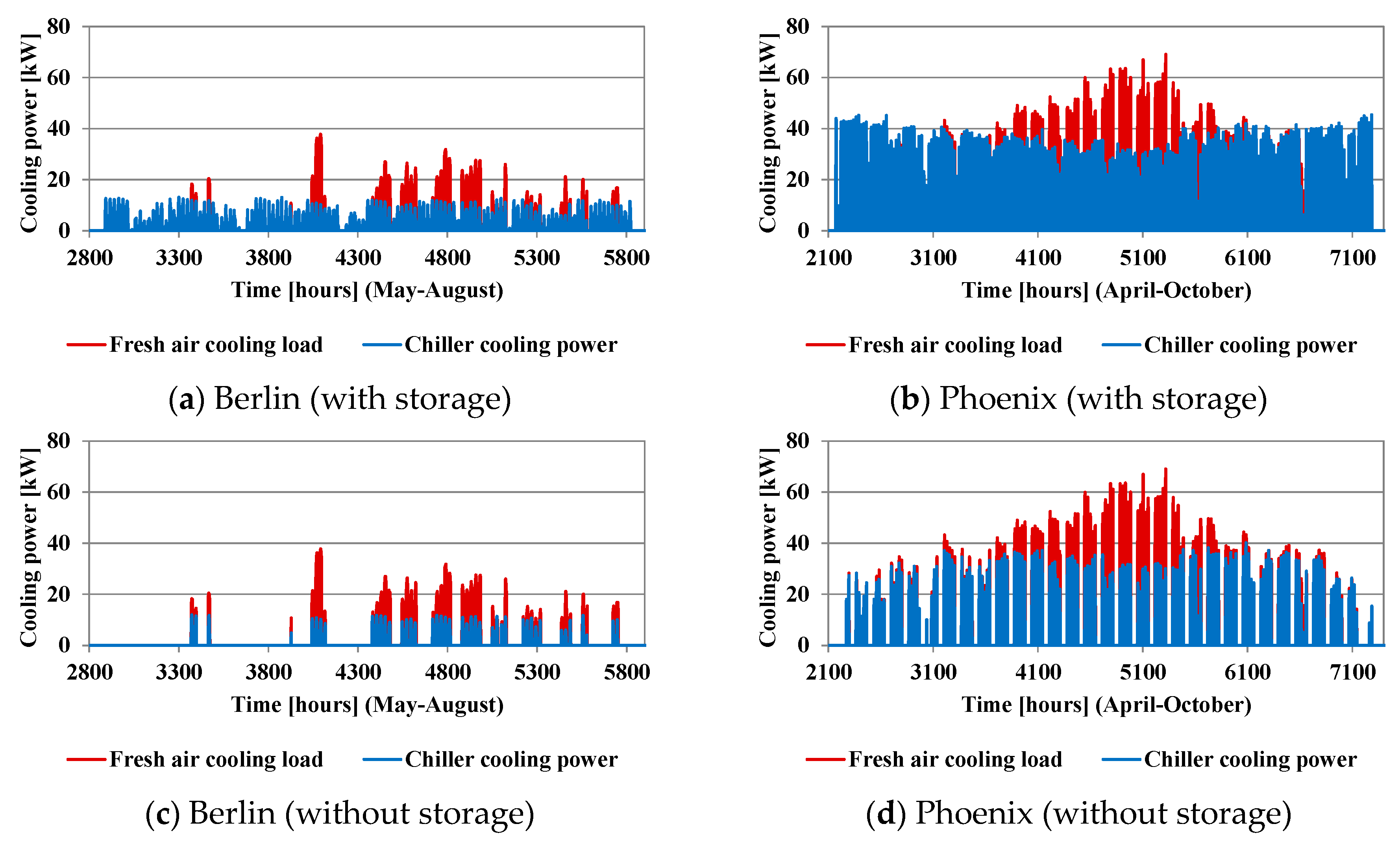
3.1. Cooling Load

Climatic conditions of each location influenced the cooling load of the considered office building.

The fresh air volume flow rate (${\dot{V}}_a$ = 7447 m³/h) was constant during the operating periods and was determined as function of number of occupants and of available floor surface [18].

The fresh air mass flow rate (${\dot{m}}_a$ (kg/s)) was determined as:

$${\dot{m}}_a={\rho }_a·{\dot{V}}_a$$

(13)

where ρ_a (kg/m³) is the air density variable with temperature and moisture.

The sensible fresh air cooling load (${\dot{Q}}_0$ (kW)) was determined as:

$${\dot{Q}}_0={\dot{m}}_a·c_a·\left(t_a-t_s\right)$$

(14)

where c_a = 1 kJ/kgK is the specific heat of the air, t_a = t_db (°C) is the ambient air (or the dry bulb) temperature, and t_s = 22 °C is the supply air temperature, considered to be constant to provide constant comfort conditions inside the building. It was considered that the inside temperature was also maintained constant (t_in = 25 °C) and fresh air cooling was required only when (t_a > t_in).

In the same conditions, the total fresh air cooling load (${\dot{Q}}_{0h}$ [kW]) was determined as:

$${\dot{Q}}_{0h}={\dot{m}}_a·\left(h_a-h_s\right)$$

(15)

where h_a and h_s are the enthalpies of the ambient air and of the supply air, respectively.

The supply air enthalpy was determined at the considered supply temperature taking into account the two possible cooling cases of ambient air—at a constant humidity ratio or with drying. If the temperature of the heat transfer surface between the chilled water and the air was higher than the dew point of the ambient air, cooling takes place at constant humidity ratio and otherwise with drying. The temperature of the heat transfer surface was 2 °C higher than the average temperature of the chilled water in the air heat exchanger of the HVAC unit.

The other components of the cooling load in the same office building, situated in different locations are presented in [18] (through the envelope, due to the occupants, due to the lightning, etc).

Table 4. Periods in which the fresh air cooling is needed and the maximum cooling load.

Location	Beginning Month	Ending Month	Max. Sensible Cooling Load (kW)	Max. Total Cooling Load (kW)
Berlin	May	August	31.30	37.84
Paris	June	September	24.68	44.00
Monaco	August	August	14.62	33.04
Rome	June	September	23.89	42.29
Seville	April	September	42.23	55.71
Cairo	April	October	46.31	46.64
Phoenix	April	October	50.75	69.09
Las Vegas	April	October	50.75	55.87

presents the periods in which the fresh air cooling was needed, the maximum sensible cooling load, and the maximum total cooling load, for each location.

The minimum value of the maximum total cooling load corresponded to Monaco and the maximum value of the maximum total cooling load corresponded to Phoenix.

The minimum values of both the maximum sensible cooling load and the maximum total cooling load corresponded to the same location—Monaco, while the maximum values of the same parameters corresponded to different locations. The maximum sensible cooling load corresponded to both Phoenix and Las Vegas and the maximum total cooling load corresponded to Phoenix.

Figure 8 presents the cooling load variation for two of the considered locations—Berlin and Phoenix.

The presented data sustains that the location considerably influenced both the cooling load and the duration of the cooling period. It could also be observed that the points of the maximum sensible and total cooling load did not occur in correspondence.

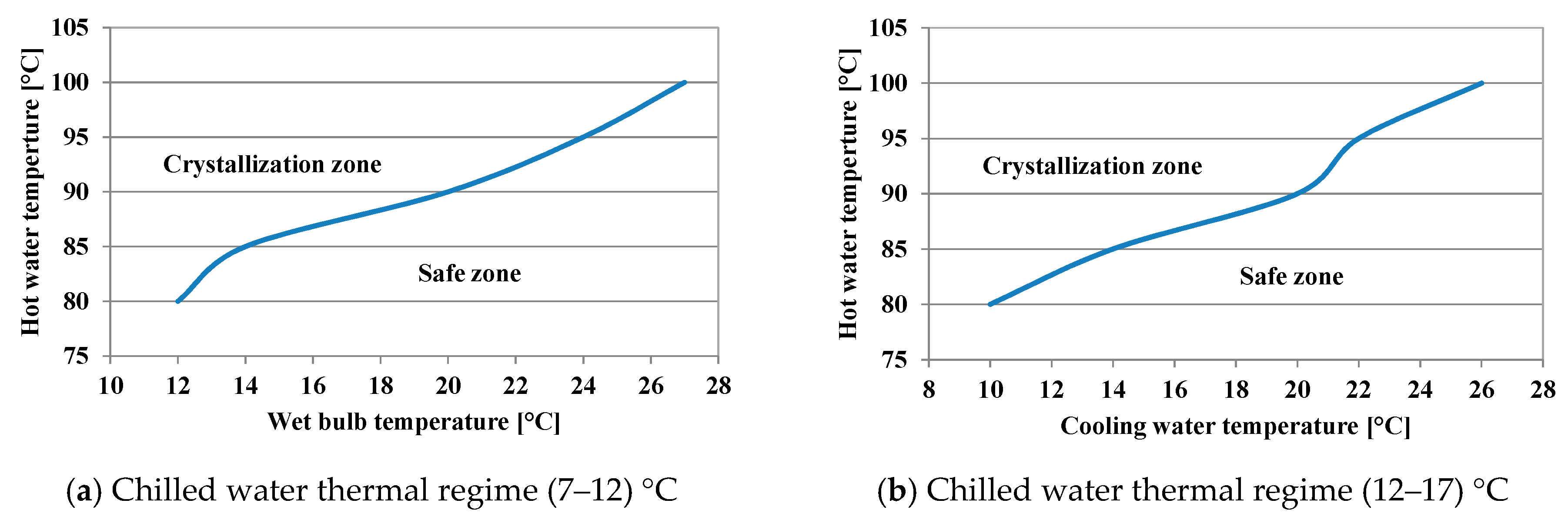
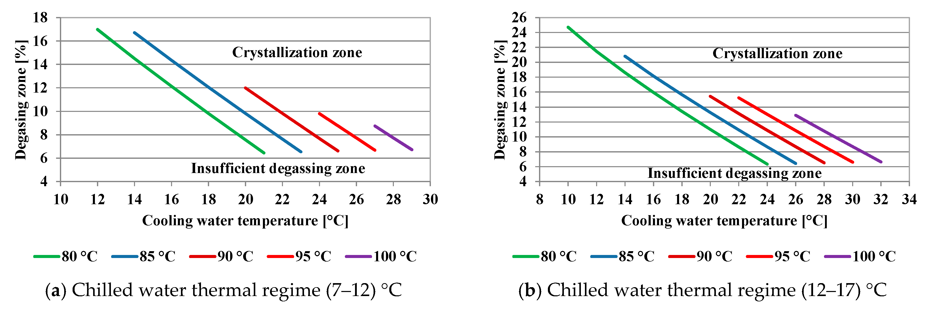
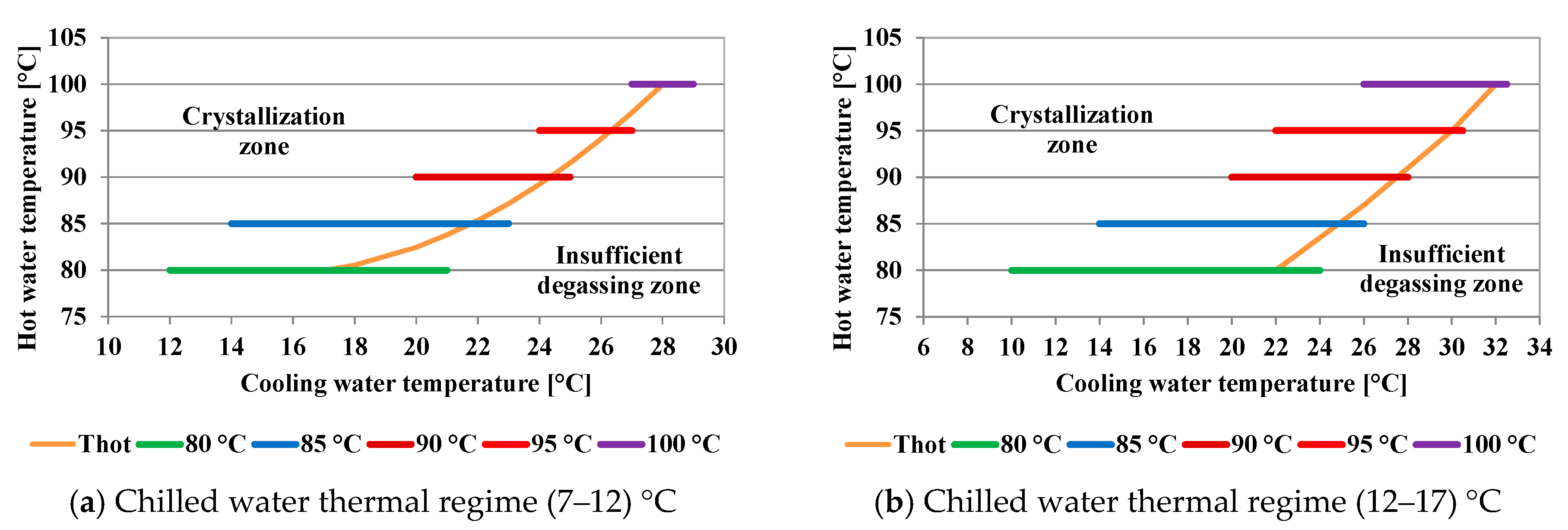
3.2. Operating Limits

The operating limits of the LiBr-H₂O absorption chiller were determined by the crystallization risk and the reduction of the degassing zone. The crystallization risk depended on the correlation between both cooling water temperature and hot water temperature. Figure 9 presents the safe zone and the crystallization zone as a function of the two mentioned temperatures for the two thermal regimes of chilled water.

The operating conditions must always be situated below the crystallization curve presented in Figure 8 and it must be correlated with the crystallization curve presented in Figure 6.

State 10 (Figure 6) was the most critical from the crystallization point of view. The position of state 10 on the enthalpy-concentration diagram was determined at the intersection between the concentration of state 6 (ζ₆ (%)) and the evaporating pressure (p₀ (bar)) (similar with the absorption pressure). The concentration of state 6 (ζ₆) at its turn, was influenced by the condensing pressure (p_k [bar]) (similar with the generator pressure) and the hot water temperature as suggested in Figure 10.

At a certain value of the condensing pressure (and of the corresponding cooling water temperature), the lower values of the hot water temperature values determined lower values of concentrations, thus reducing the risk of crystallization.

At a certain value of the hot water temperature, the higher values of the condensing pressure (and of the corresponding cooling water temperature) determine lower values of concentrations, thus reducing the risk of crystallization.

It can be concluded that low values of cooling water temperatures (low values of condensing pressure) should be associated with lower values of hot water temperatures to avoid the risk of crystallization. Similarly, high values of cooling water temperatures (high values of condensing pressure) should be associated with higher values of hot water temperatures to avoid the risk of crystallization. This interdependence between the cooling water temperature and the hot water temperature to avoid the risk of crystallization is presented in Figure 9.

The influence of the cooling water temperature on the degassing zone for different hot water temperatures is presented on Figure 11.

The degassing zone decreased with increasing cooling water temperatures (equal with the wet bulb temperature). The upper limits of each line on the chart represent the crystallization limit for each hot water temperature. Each line, corresponding to different hot water temperatures, presents as the left limit—the minimum cooling water temperature that avoids crystallization, and as right limit-—the maximum cooling water temperature corresponding to the minimum accepted degassing zone.

Since the concentration of states 10 and 6 (ζ₁₀ = ζ₆) was determined as it was presented, the degassing zone was determined by the concentration of states 8 and 1 (ζ₈ = ζ₁), respectively on the concentration of the diluted solution. The influence of the cooling water and the chilled water temperatures on the diluted solution concentration is presented in Figure 12.

At a certain value of evaporating pressure (and of the corresponding chilled water temperature), lower condensing temperature values (and of the corresponding cooling water temperature) determined lower values of the diluted solution concentration and higher values of the degassing zone.

At a certain value of condensing temperature (and of the corresponding cooling water temperature), higher evaporating pressure values (and of the corresponding chilled water temperature) determined lower values of the diluted solution concentration and higher values of the degassing zone.

It can be concluded that if the chilled water temperature and thus the evaporating pressure was constant, and if the hot water temperature was also known (and determined in such a manner as to eliminate the risk of crystallization), then low values of condensing temperature (and of the corresponding cooling water temperature) determines lower values of the diluted solution concentration and higher values of the degassing zone.

Since the operating conditions must satisfy both conditions of no crystallization and sufficient degassing zone, the hot water temperature must be correlated with the cooling water temperature in order to satisfy both restrictions. Thus, at a certain value of the hot water temperature, there exists a lower value of the cooling water temperature limited by the crystallization risk and a higher value of the cooling water temperature limited by the minimum required degassing zone.

It can be observed that the degassing zone decreased with increasing cooling water temperature. The upper limits of each line on the chart represent the crystallization limit for each hot water temperature. Each line, corresponding to different hot water temperatures, presents as the left limit—the minimum cooling water temperature that avoids crystallization, and as the right limit—the maximum cooling water temperature corresponding to the minimum accepted degassing zone.

Figure 13 presents the acceptable operating ranges from the cooling water and hot water temperatures’ point of view.

Since the acceptable operation zone depended on both the hot water and the cooling water temperatures, the dependence between the hot water and the cooling water temperatures was established and represented on the chart. The original correlation for the solar hot water temperature (t_h (°C)) as function of the cooling water temperature (t_w (°C)) to ensure acceptable operating conditions was:

$$t_h=a·t_w^2-b·t_w+c$$

(16)

The coefficients of the hot water temperature correlation are presented in

Table 5. The coefficients of the hot water temperature correlation.

Chilled Water Thermal Regime	Correlation Coefficients			Availability Range (Cooling Water Thermal Regime)
	a	b	c
(7–12) °C	0.1233	3.7314	107.76	(17–28) °C
(12–17) °C	0.0424	0.3116	66.18	(10–32) °C

.

The availability range of this correlation is of t_w = (17–28) °C. The hot water temperature at the outlet of the solar thermal system should be constant at 80 °C, with the cooling water temperature in the range of t_w = (12–17) °C. If the cooling water temperature at the outlet of the cooling tower decreased below 12 °C due to the actual operating conditions, the cooling tower must be regulated in order to maintain the outlet cooling water temperature higher than 12 °C.

Figure 14 presents the variation of the cooling water temperature at the outlet of the cooling tower.

The difference between the cooling water temperature at the outlet of the cooling tower and the wet bulb temperature of the ambient air at the inlet in the cooling towers was 5 °C, which is in agreement with similar values reported in the literature. This parameter was considered in the range of (3.2–4.8) °C in [29], and in the range of (1.5–5.5) °C in [30]. The wet bulb temperature variation, used to determine the cooling water temperature variations presented in Figure 14, was taken from the TMY as previously mentioned.

Figure 15 presents the variation of the required solar hot water temperature with time, determined by the cooling water temperature variation, for two of the considered locations—Berlin and Phoenix.

The higher values of solar hot water temperature corresponded to the higher values of cooling water temperature. The variations of the solar hot water temperature presented in Figure 15 were determined by using the correlation provided in Equation (16).

The minimum outlet solar hot water temperature is 80 °C for all locations. The maximum outlet solar hot water temperature is 100 °C for all locations except for Cairo for which the value is of 96 °C.

Similar values are reported in the literature for the solar hot water temperature 80–90 °C [28], 55–135 °C [8], 90–100 °C [15], 85–90 °C [31], and 84–120 °C [14].

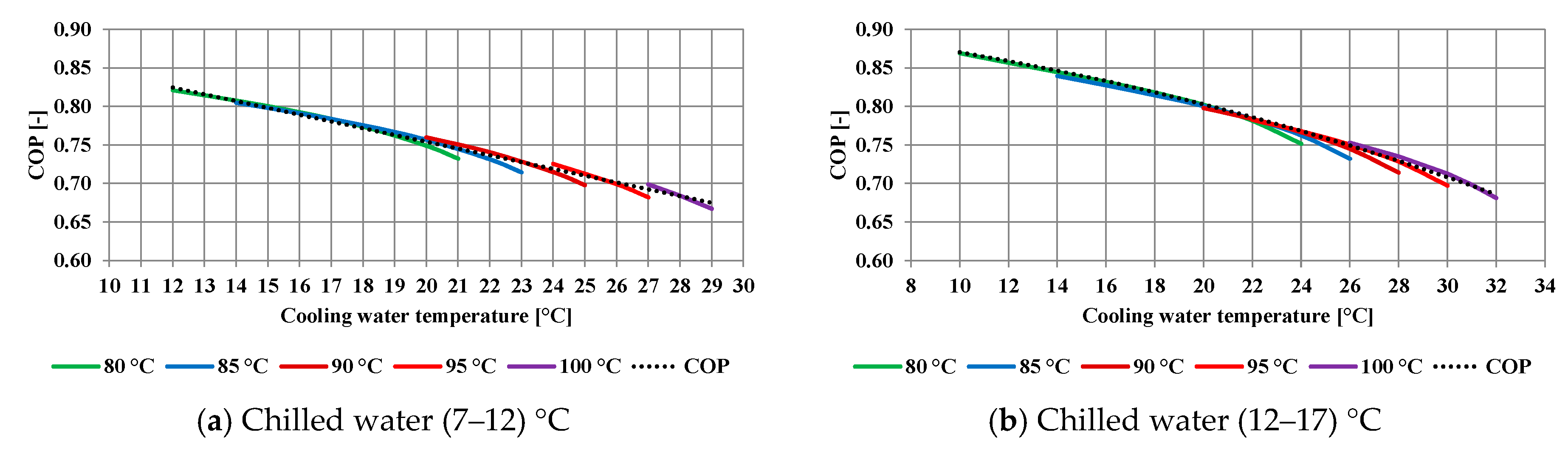
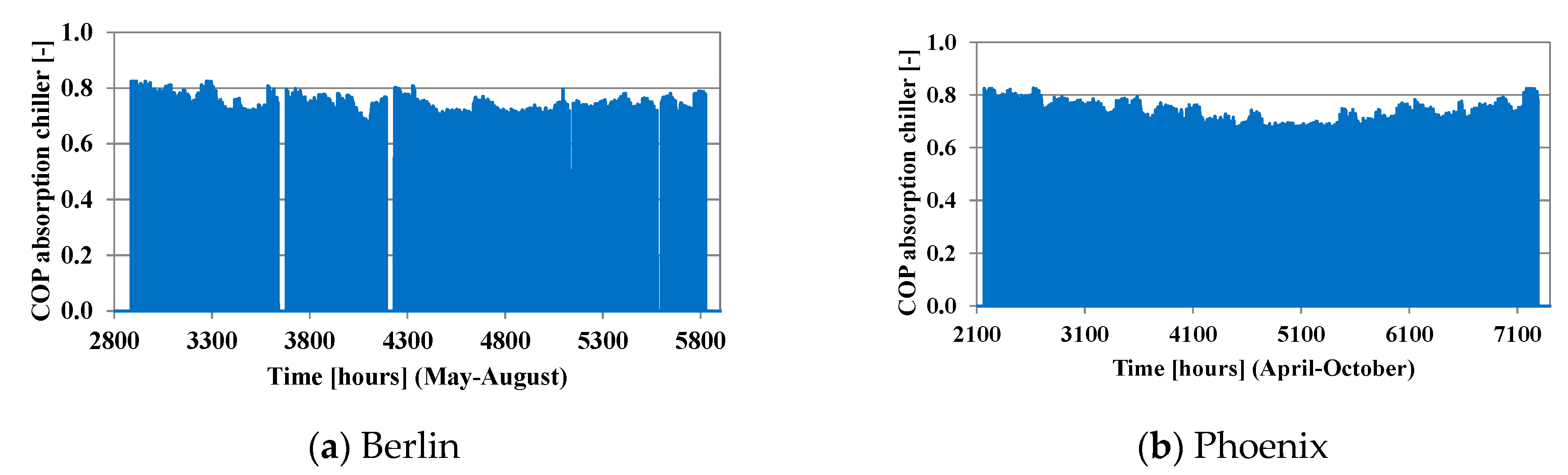
3.3. COP of the Solar Absorption Chiller and of the Electric Chiller

The COP depends on the thermal regimes of the three connected circuits: cooled water; hot water and cooling water. Since the chilled water thermal regime is constant at (7–12) °C or (12–17) °C, COP depends only on the cooling water temperature and on the hot water temperature that at its turn must be correlated with the cooling water temperature.

Figure 16 presents the variation curves of COP with the cooling water temperature for different hot water temperatures.

For each hot water temperature in the range of (80–100) °C the cooling water temperature was considered in the acceptable variation range. The dotted line presents the COP variation with the cooling water temperature. This variation also includes the hot water dependence on the cooling water.

The correlations for the COP as a function of the cooling water temperature that includes the hot water temperature dependence on the same cooling water temperature (COP = f(t_w,t_h(t_w) = f(t_w)) was determined as:

$$COP=a·t_w^2+b·t_w+c$$

(17)

The coefficients of the COP correlations are presented in

Table 6. COP correlation coefficients.

Chilled Water Thermal Regime	Correlation Coefficients			Availability Range (Cooling Water Thermal Regime)
	a	b	c
(7–12) °C	0.0	−0.0088	0.93	(17–28) °C
(12–17) °C	−0.000135	−0.0027	0.9107	(10–32) °C

.

Figure 17 presents the COP variation as a function of time, for two of the considered locations: Berlin and Phoenix.

The higher values of the COP correspond to the lower values of the cooling water and solar hot water temperatures.

The COP values are in good agreement with the ones reported in the literature: 64–76% [31], 71–84% [10], 80% [8], 40–80% [9].

The electric power needed to run the electric chiller (P_el (kW)) was determined as:

$$P_{el}=\frac{{\dot{Q}}_{0,deficit}}{CO{P}_{el}}$$

(18)

where ${\dot{Q}}_{0,deficit}$ (kW) is the difference between the cooling load and the cooling power of the absorption chiller.

The solar fraction (SF (%)) was defined as the ratio between the cooling power and the cooling load:

$$SF=\frac{{\dot{Q}}_0}{{\dot{Q}}_{0h}}$$

(19)

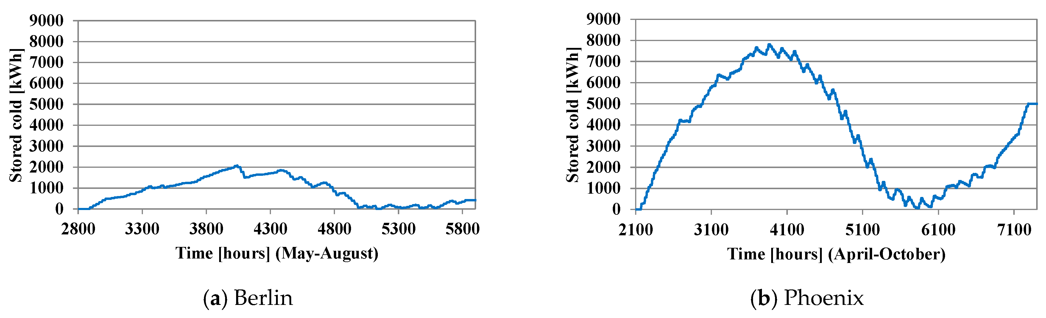
3.4. Effect of Chilled Water Storage

If the SFACS includes a chilled water storage tank (cold storage), several characteristics of the system can be modified: number (or area) of the ETSC; maximum cooling power of the absorption chiller, etc.

In this study, the ETSC field was designed for each location to completely eliminate the electric chiller when chilled water storage is present. The behaviors of the SFACS with the same ETSC field but without storage are also presented. With storage, the absorption chiller can operate and cumulate cold, even when fresh air cooling is not needed. The main advantage of the cold storage is the possibility to reduce the maximum cooling power considerably under the cooling load and furthermore the dimensions of the ETSC field.

The problem of sizing the chilled water storage was not approached in this study. It was simply considered that if the cooling power of the SFACS is higher than the cooling load, the exceeding cooling load can be stored as chilled water, to be used when the cooling load exceeds the cooling power.

Figure 18 presents the cooling power and the total cooling load with and without storage in comparison to the cooling load, for two of the considered locations: Berlin and Phoenix.

The fresh air cooling loads, presented in Figure 18, were determined based on Equation (15) and the cooling powers, presented in the same Figure, were determined as the product between the COP and the solar heating power (equal with the thermal power of the generator) as stated in Equation (11). At its turn, the COP was determined based on the correlation provided in Equation (17).

Solar cooling with storage was always provided when solar radiation was available, even if the building did not require cooling, as presented in Figure 18a,b. Solar cooling without storage was provided only if the building required cooling and if solar radiation was available, as presented in Figure 18c,d.

Figure 19 presents the evolution of the stored cold for two of the considered locations—Berlin and Phoenix.

It can be observed that the cold accumulated in periods with a lower cooling load was used in the periods with a high cooling demand in such a manner that there were no periods with a cold deficit. This was the dimensioning criteria for the ETSC field. The number of ETSC for each location is the minimum number that assured no cooling deficit.

When cold was accumulated, the trend of the curves presented in Figure 19 was ascendant, while when the stored cold was used, the trend of the curves presented in Figure 19 was descendent

The produced cooling power was higher in some periods and lower in other periods in comparison to the required cooling load. Using storage, the cold deficit was always avoided, and the seasonal cold balance was such that the SFACS always produced more cooling than required, meaning that the seasonal solar fraction was always higher than 100%.

Figure 20 presents the instantaneous solar fraction without storage, for the two locations.

Since the SFACS are designed to operate with storage and thus with reduced cooling power, without storage the total cooling load could only be completely covered by the absorption chiller (solar fraction a 100%) in periods with reduced cooling load and high solar radiation.

The cooling power (chilled water), the solar heating power, and the cooling power of the cooling tower as the main components of the thermal energy balance of the SFACS are presented in Figure 21 for both of the considered locations—Berlin and Phoenix.

The thermal energy balance of the SFACS highlight that the sum of the entered thermal powers (the cooling power of the evaporator and the thermal power of the generator) was equal to the sum of the evacuated thermal powers (of the absorber and of the condenser). The thermal power of the generator was equal to the solar heating power of the ETSC and the sum between the thermal powers of the absorber and of the condenser represented the thermal power of the cooling tower. Thus, the cooling power of the cooling tower was always equal to the sum between the provided cooling power and the solar heating power, while the cooling power was always lower than the solar heating power, the ratio between the two parameters being the COP.

It can also be observed that the amount of the thermal balance components are about four times higher in Phoenix than the corresponding values in Berlin.

Table 7. Characteristics of the SFACS for each location.

Location	Berlin	Paris	Monaco	Rome	Seville	Cairo	Phoenix	Las Vegas
No. of ETSC (pcs)	14	12	18	28	30	29	44	32
Total aperture surface (m2)	26.1	22.4	33.6	52.2	55.9	54.1	82.0	59.6
Max. cooling load (kW)	37.84	44.00	33.04	42.29	55.71	46.64	69.09	55.87
No. of operating hours at (12–17) °C chilled water (h)	0	0	121	25	32	0	157	4
Max. absorption cooling power (with storage) (kW)	13.15	10.75	14.70	23.89	26.86	30.26	45.29	33.48
Max. absorption cooling power (without storage) (kW)	11.99	10.40	14.41	22.36	26.46	29.62	40.06	30.86
Electrical power (with storage) (kW)	0.0	0.0	0.0	0.0	0.0	0.0	0.0	0.0
Max. electrical power (without storage) (kW)	9.10	11.58	9.56	10.14	12.72	6.73	18.04	13.67
Total cooling load (seasonal) (MWh)	6.14	2.56	2.09	12.74	24.18	31.79	41.90	31.07
Seasonal solar fraction (with storage) (%)	106.8%	176.9%	114.4%	121.0%	102.9%	109.9%	111.9%	115.8%
Seasonal solar fraction (without storage) (%)	35.7%	29.5%	35.3%	57.2%	52.4%	57.4%	62.0%	53.9%
Seasonal electric fraction (without storage) (%)	64.3%	70.5%	64.7%	42.8%	47.6%	42.6%	38.0%	46.1%
Total electrical energy (with storage) (kWh)	0.0	0.0	0.0	0.0	0.0	0.0	0.0	0.0
Total electrical energy (without storage) (kWh)	955.7	465.0	382.3	1455.0	1048.2	2261.6	4192.3	3431.8
Seasonal energy efficiency ratio (electric) (SEERel) (-)	4.1	3.9	3.5	3.7	3.8	6.0	3.8	4.2
Seasonal energy efficiency ratio (global) (SEERgl) (-)	6.4	5.5	5.5	8.8	8.8	14.1	10.0	9.1

presents some characteristics of the SFACS for each location.

Several observations can be made by analyzing the comparative data concerning the SFACS.

The climate type was not sufficient to provide a guideline concerning the SFACS. Calculations were always needed and should be based on the particular local climate or meteorological data. In this study the TMY data was used. For example, locations with similar climate types (Cairo and Phoenix) were characterized by a different maximum cooling load (46.64 kW and 69.09 kW, respectively), by a different maximum cooling power of the absorption chiller in both operating situations—(with cold storage 30.26 kW and 45.29 kW, respectively) or (without cold storage 29.62 kW and 40.06 kW, respectively), and by a different number of ETCS (29 and 44, respectively), etc. As another example, even if situated in different climate zones, the characteristics of the SFACS in Seville and Cairo were almost similar. Another comparison can be carried out between Seville and Cairo. In Seville the number of ECTS (30) was higher than Cairo (29), but the provided cooling power with and without storage was lower than Cairo (26.86 kW vs. 30.26 kW with storage and 26.46 kW vs. 29.62 kW without storage).

The major benefit of using the cold storage tank was that on one hand it could reduce the required cooling power and furthermore the size of ECTS field, and on the another hand, it did not require the electric chiller and its electrical energy consumption.

It can be observed that the values of the maximum absorption cooling power with storage were higher than the values of the maximum absorption cooling power without storage for all of the considered locations. This occurs due to the fact that with storage there were more operating periods than without storage and if the number of operating periods increased then the chance to reach more favorable operating conditions also increased, with high solar radiation and high COP.

Without cold storage, the SFACS couldn’t provide enough cooling power to cover the whole cooling demand. Thus, when the cooping power provided by the SFACS was insufficient, the operation of the electric chiller was required.

Depending on the local meteorological conditions, the characteristics of the SFACS varies considerably:

-

The number of ETCS varied from 12 in Paris up to 44 in Phoenix and the corresponding total aperture area varied from 22.4 m² in Paris to 82.0 m² in Phoenix;

-

The total seasonal cooling load represents the total required cooling energy. This parameter was calculated hourly as the product between the cooling load (thermal power) and the period of time when cold was required. The sum of the hourly required cooling energy represents the total seasonal cooling load and varied between 2.09 MWh in Monaco up to 41.90 MWh in Phoenix.

-

The cooling power of the absorption chiller with cooling storage varied from 10.75 kW in Paris up to 45.29 kW in Phoenix;

-

The cooling power of the absorption chiller without cooling storage varied from 10.40 kW in Paris up to 40.06 kW in Phoenix;

-

The cooling storage proved to be capable of covering the cooling load without the electric chiller and the corresponding electrical energy consumption;

-

The maximum required electric power of the electric chiller, without storage varied between 6.73 kW in Cairo up to 18.04 kW in Phoenix;

-

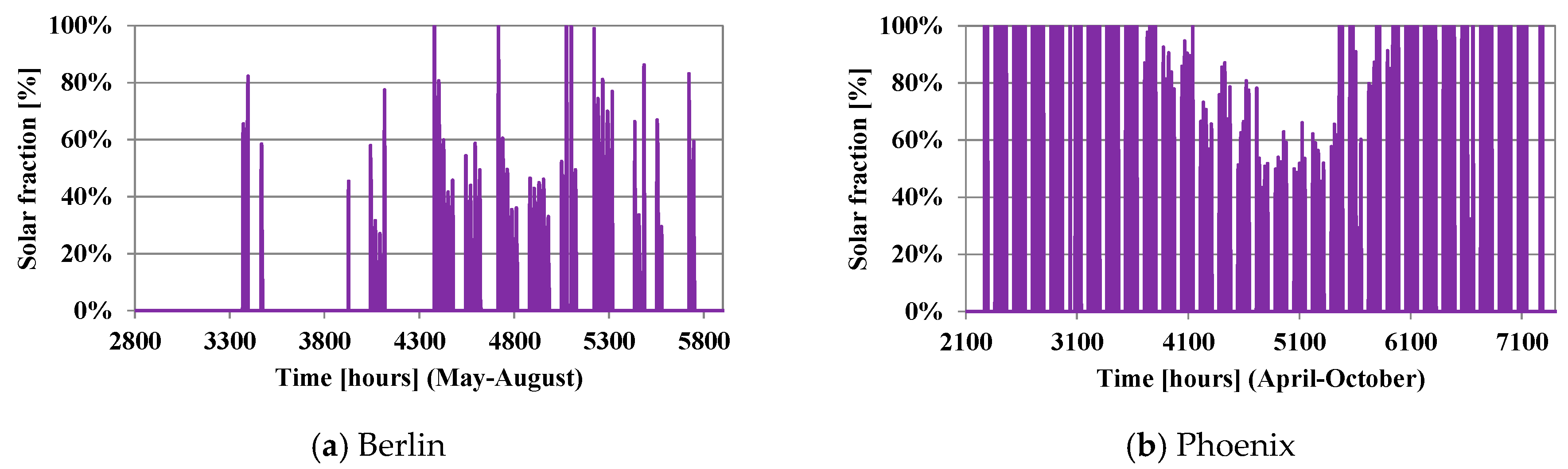
The seasonal solar fraction with storage was higher than 100%, meaning that with storage more cold could be produced than required for the fresh air cooling, the extra cold production being, possibly, used to cover other types of cooling loads inside the building (through envelope, from occupants, from lighting, etc.);

-

The seasonal solar fraction without storage varied between 29.5% in Paris up to 62.0% in Phoenix;

-

The total amount of electrical energy required without storage was situated in the range of 382.3 kW (Monaco) up to 4192.3 kW (Phoenix);

-

The seasonal energy efficiency ratio (SEER) represents the ratio between the seasonal provided cold and the total required seasonal electrical energy. Two types of SEER were defined—(a) the electrical seasonal energy efficiency ratio (SEERel) calculated considering only the electrical provided cold; and (b) the global seasonal energy efficiency ratio (SEERgl) considering the whole amount of provided cold (solar + electric). SEERel was between 3.5 in Monaco and 6.0 in Cairo. SEERgl was between 5.5 in Paris or Monaco and 14.1 in Cairo.

4. Conclusions

The study presents a new perspective to the SFACS serving an office building placed in different climatic conditions, carried out by simulation. The complete analytical mathematical model of the SFACS thermal behavior was presented in detail. The presented results refer to both operating conditions and parameters of performance.

The standard thermal regime of the chilled water circuit in the absorption chiller was (7–12) °C, similar to that of classical electric chillers. If the operating conditions of the absorption chiller became incompatible with this thermal regime, an alternative chilled water thermal regime of (12–17) °C was proposed. In Berlin, Paris, and Cairo the operating conditions always allowed the chilled water to operate at the thermal regime of (7–12) °C. In Las Vegas the chilled water thermal regime of (12–17) °C was needed for only 4 h, while this thermal regime was required for 25 h in Rome, 32 h in Seville, 121 h in Monaco, and 157 h in Phoenix.

New correlations between the solar hot water temperature and the cooling water temperature were proposed for two thermal regimes of the chilled water, in order to avoid both crystallization and the reduction of the degassing zone below 6%.

New correlations between the COP variation of the LiBr-H₂O absorption chiller and the cooling water temperature were proposed for two thermal regimes of the chilled water. These variations also embed the solar hot water temperature variation as a function of the same cooling water temperature.

Based on the SFACS mathematical model, its thermal behavior was simulated considering the system located in different locations with different climatic conditions.

It was highlighted that the local climatic particularities determined very different characteristics of the SFACS:

The maximum cooling load varied between 33.04 kW in Monaco to 69.09 kW in Phoenix;

The number of ETSC varied from 12 in Paris to 44 in Phoenix;

The maximum values of the LiBr-H₂O absorption chiller COP, varied from 76.5% for Monaco and 79.3% for Rome to 82.4% for the rest of considered locations.

It was found that using a cold storage tank affected many characteristics of the SFACS:

The seasonal electrical energy consumption for fresh air cooling could be reduced up to 0 kWh;

The need of using a peek load electrical chiller could be eliminated, and the solar fraction of the fresh air cooling load could be increased from (29.5–62.0)% without cold storage (depending on the location) to more than 100% and the exceeding cold could be used to partially cover other types of cooling loads of the building—through the envelope, from the lighting system, and from occupants, etc.

Future work can be focused on the limits and performances of air cooled SFACS, on the dimensioning of the storage tank, and on the SFACS optimization depending on the storage tank volume.

References

1. Directive/31/EU, Directive 2010/31/EU of the European Parliament and of the Council of 19 May 2010 on the Energy Performance of Buildings in 2010. Available online: https://www.google.com.tw/url?sa=t&rct=j&q=&esrc=s&source=web&cd=1&cad=rja&uact=8&ved=2ahUKEwi3mvHtsMriAhUVPnAKHYpUDAAQFjAAegQIBhAC&url=https%3A%2F%2Feur-lex.europa.eu%2FLexUriServ%2FLexUriServ.do%3Furi%3DOJ%3AL%3A2010%3A153%3A0013%3A0035%3AEN%3APDF&usg=AOvVaw0pOZGXaqo5VZyusosxfeop (accessed on 7 April 2019).
2. Wei, Y.; Zhang, X.; Shi, Y.; Xia, L.; Pan, S.; Wu, J.; Han, M. A review of data-driven approaches for prediction and classification of building energy consumption. Renew. Sustain. Energy Rev. 2018, 82, 1027–1047. [Google Scholar] [CrossRef]
3. Roaf, S.; Brotas, L.; Nicol, F. Counting the costs of comfort. Build. Res. Inf. 2015, 43, 269–273. [Google Scholar] [CrossRef]
4. Mammoli, A.; Vorobieff, P.; Barsun, H.; Burnett, R.; Fisher, D. Energetic, economic and environmental performance of a solar-thermal-assisted HVAC system. Energy Build. 2010, 42, 1524–1535. [Google Scholar] [CrossRef]
5. Wang, J.; Yan, R.; Wang, Z.; Zhang, X.; Shi, G. Thermal Performance Analysis of an Absorption Cooling System Based on Parabolic Trough Solar Collectors. Energies 2018, 11, 2679. [Google Scholar] [CrossRef]
6. Ma, Y.; Saha, S.C.; Miller, W.; Guan, L. Comparison of Different Solar-Assisted Air Conditioning Systems for Australian Office Buildings. Energies 2017, 10, 1463. [Google Scholar] [CrossRef]
7. Chan, J.J.; Best, R.; Cerezo, J.; Barrera, M.A.; Lezama, F.R. Experimental Study of a Bubble Mode Absorption with an Inner Vapor Distributor in a Plate Heat Exchanger-Type Absorber with NH3-LiNO3. Energies 2018, 11, 2137. [Google Scholar] [CrossRef]
8. Cerezo, J.; Romero, R.J.; Ibarra, J.; Rodríguez, A. Dynamic Simulation of an Absorption Cooling System with Different Working Mixtures. Energies 2018, 12, 259. [Google Scholar] [CrossRef]
9. Sarbu, I.; Sebarchievici, C. Review of solar refrigeration and cooling systems. Energy Build. 2013, 67, 286–297. [Google Scholar] [CrossRef]
10. Manu, S.; Chandrashekar, T.K. A simulation study on performance evaluation of single-stage LiBr-H2O vapor absorption heat pump for chip cooling. Int. J. Sustain. Built Environ. 2016, 5, 370–386. [Google Scholar] [CrossRef]
11. Patel, H.A.; Patel, L.N.; Jani, D.; Christian, A. Energetic analysis of single stage lithium bromide water absorption refrigeration system. Procedia Technol. 2016, 23, 488–495. [Google Scholar] [CrossRef]
12. Farnós, J.; Papakokkinos, G.; Castro, J.; Morales, S.; Oliva, A. Dynamic Modelling of an Air-Cooled LiBr-H2O Absorption Chiller Based on Heat and Mass Transfer Empirical Correlations. Available online: https://www.google.com.tw/url?sa=t&rct=j&q=&esrc=s&source=web&cd=1&ved=2ahUKEwirvLucscriAhUN-2EKHRJ7B8EQFjAAegQIBhAC&url=https%3A%2F%2Fhpc2017.org%2Fwp-content%2Fuploads%2F2017%2F06%2Fo454.pdf&usg=AOvVaw1CSUoj6w0EocuFqv91wyTW (accessed on 7 April 2019).
13. Stanciu, C.; Stanciu, D.; Gheorghian, A.T.; Tanase, E.B.; Dobre, C.; Spiroiu, M. Maximum Exergetic Efficiency Operation of a Solar Powered H2O-LiBr Absorption Cooling System. Entropy 2017, 19, 676. [Google Scholar] [CrossRef]
14. Lizarte, R.; Izquierdo, M.; Marcosc, J.D.; Palacios, E. Experimental comparson of two solar-driven air-cooled LiBr/H2O absorption chillers: Indirect versus direct air-cooled system. Energy Build. 2013, 62, 323–334. [Google Scholar] [CrossRef]
15. Chen, J.F.; Dai, Y.J.; Wang, R.Z. Experimental and analytical study on an air-cooled single effect LiBr-H2O absorption chiller driven by evacuated glass tube solar collector for cooling application in residential buildings. Sol. Energy 2017, 151, 110–118. [Google Scholar] [CrossRef]
16. Salehi, S.; Yari, M.; Mahmoudi, S.M.S.; Farshi, L.G. Investigation of crystallization risk in different types of absorption LiBr/H2O heat transformers. Ther. Sci. Eng. Prog. 2019, 10, 48–58. [Google Scholar] [CrossRef]
17. Porumb, R.; Porumb, B.; Balan, M.C. Numerical investigation on solar absorption chiller with LiBr-H2O operating conditions and performances. Energy Procedia 2017, 112, 108–117. [Google Scholar] [CrossRef]
18. Pop, O.G.; Fechete Tutunaru, L.; Bode, F.; Abrudan, A.C.; Balan, M.C. Energy efficiency of PCM integrated in fresh air cooling systems in different climatic conditions. Appl. Energy 2018, 212, 976–996. [Google Scholar] [CrossRef]
19. Todoran, T.P.; Balan, M.C. Long term behavior of a geothermal heat pump with oversized horizontal collector. Energy Build. 2016, 133, 799–809. [Google Scholar] [CrossRef]
20. Porumb, B.; Balan, M.C.; Porumb, R. Potential of indirect evaporative cooling to reduce the energy consumption in fresh air conditioning applications. Energy Procedia 2016, 85, 433–441. [Google Scholar] [CrossRef]
21. Badescu, V.; Laaser, N.; Crutescu, R. Warm season cooling requirements for passive buildings in Southeastern Europe (Romania). Energy 2010, 35, 3284–3300. [Google Scholar] [CrossRef]
22. Badescu, V.; Laaser, N.; Crutescu, R.; Crutescu, M.; Dobrovicescu, A.; Tsatsaronis, G. Modeling, validation and time-dependent simulation of the first large passive building in Romania. Renew. Energy 2011, 36, 142–157. [Google Scholar] [CrossRef]
23. Duffie, J.A.; Beckman, W.A. Solar Engineering of Thermal Processes; Wiley&Sons: Singapore, 1980. [Google Scholar]
24. Quaschning, V. Understanding Renewable Energy Systems; Earthscan: London, UK, 2007. [Google Scholar]
25. Unguresan, P.V.; Porumb, R.A.; Petreus, D.; Pocola, A.G.; Pop, O.G.; Balan, M.C. Orientation of Facades for Active Solar Energy Applications in Different Climatic Conditions. J. Energy Eng. 2017, 143, 04017059. [Google Scholar] [CrossRef]
26. Prieto, A.; Knaack, U.; Auer, T.; Klein, T. Feasibility Study of Self-Sufficient Solar Cooling Façade Applications in Different Warm Regions. Energies 2018, 11, 1475. [Google Scholar] [CrossRef]
27. Unguresan, P.; Petreus, D.; Pocola, A.; Balan, M. Potential of solar ORC and PV systems to provide electricity under Romanian climatic conditions. Energy Procedia 2016, 85, 584–593. [Google Scholar] [CrossRef]
28. Porumb, R.; Porumb, B.; Balan, M. Baseline evaluation of potential to use solar radiation in air conditioning applications. Energy Procedia 2016, 85, 442–451. [Google Scholar] [CrossRef]
29. Syed, A.; Izquierdo, M.; Rodriguez, P.; Maidment, G.; Missenden, J. A novel experimental investigation of a solar cooling system in Madrid. Int J. Refrig. 2005, 28, 859–871. [Google Scholar] [CrossRef]
30. Stanford, H.W., III. HVAC Water Chillers and Cooling Towers. Fundamentals, Application, and Operation; Marcel Dekker: New York, NY, USA, 2003. [Google Scholar]
31. Chen, J.F.; Dai, Y.J.; Wang, H.B.; Wang, R.Z. Experimental investigation on a novel air-cooled single effect LiBr-H2O absorption chiller with adiabatic flash evaporator and adiabatic absorber for residential application. Sol. Energy 2018, 159, 579–587. [Google Scholar] [CrossRef]
Figure 1. The 3D drawing of the building equipped with solar thermal collectors.
Energies 12 02113 g001
Figure 2. Global solar radiation on horizontal plane and ambient temperature.
Energies 12 02113 g002
Figure 3. Energy flow scheme of a solar absorption fresh air cooling system.
Energies 12 02113 g003
Figure 4. The principle scheme of the LiBr-H2O solar absorption chiller.
Energies 12 02113 g004
Figure 5. The working cycle of the main refrigerating circuit.
Energies 12 02113 g005
Figure 6. The working cycle of the LiBr-H2O solution.
Energies 12 02113 g006
Figure 7. ETSC thermal efficiency for the two locations.
Energies 12 02113 g007
Figure 8. Cooling load variation for two considered locations.
Energies 12 02113 g008
Figure 9. Safe zone and crystallization zone.
Energies 12 02113 g009
Figure 10. Influence of different parameters on the risk of crystallization.
Energies 12 02113 g010
Figure 11. Influence of the cooling water and hot water temperature on the degassing zone.
Energies 12 02113 g011
Figure 12. Influence of different parameters on the diluted solution concentration.
Energies 12 02113 g012
Figure 13. Acceptable operating ranges.
Energies 12 02113 g013
Figure 14. The variation of the cooling water temperature for two locations.
Energies 12 02113 g014
Figure 15. The variation of the required solar hot water temperature for two locations.
Energies 12 02113 g015
Figure 16. Variation of COP with the cooling water temperature and with hot water temperatures.
Energies 12 02113 g016
Figure 17. The COP variation for two locations.
Energies 12 02113 g017
Figure 18. The cooling power with and without storage for two locations.
Energies 12 02113 g018
Figure 19. The stored cold.
Energies 12 02113 g019
Figure 20. Variation of instantaneous solar fraction without storage.
Energies 12 02113 g020
Figure 21. The main components of the SFACS thermal energy balance.
Energies 12 02113 g021