The Influence of Changing Hydropower Potential on Performance Parameters of Pumps in Turbine Mode

Abstract

Pumps as turbines (PAT) are used as an alternative to water turbines in small hydropower plants. The same devices can also be used for energy recovery in water distribution networks. They can replace pressure reduction valves that often lead to energy loss. However, PATs lack the parts that regulate flow so that when a hydropower potential change occurs, efficiency is reduced, as is economic gain. This article summarizes the influence of changing hydropower potential on PAT efficiency and presents comparisons of experimental results with the commonly used predictive model stemming from the theory of physical similarity, which presumes constant PAT efficiency. Our research indicates that the deviation between the model and the real power output calculation at varying potentials was minimal. Similarly, the affine parabola can be used to determine the relationship between total head and flow rate. Other relationships differ from reality the more the PAT efficiency changes. The flow rate and total head dependence on shaft speed are the main factors when setting the optimum operational parameters at varying hydropower potentials. Therefore, a change in efficiency must be included in predictive calculations to correctly optimize PAT operation. The problem is that a change in efficiency cannot be reliably predicted in advance, especially in the case of small-scale devices. For this reason, further research on the issue of changes in PAT efficiency is necessary.

1. Introduction

The interest in pumps as turbine (PAT) technology has been revived in recent decades. It has been significantly used in power supply installations in remote areas, both on- and off-grid. The use of hydraulic pumps operating as turbines offers several advantages with respect to conventional turbines. The major advantages are its low investment costs and market accessibility. Small centrifugal pumps operating as turbines with an output of 5 kW or less are also a low-cost alternative to crossflow turbines even in small hydropower plants.

Giosio et al. [1] and Williams [2] mentioned industrial applications of PATs in energy recovery systems where a high-pressure water source exists that would otherwise require throttling. Pugliese et al. [3] indicated that the excess head can be exploited for hydropower generation by using turbines and/or PATs. They refer to PATs as pumps running in reverse mode by inverting the flow direction and using the electric motor as a generator. The possibility of using pumps operating in turbine mode has been widely accepted since the third decade of the 20th century, but the benefit of their use in water distribution networks (WDNs) has only been pointed out in recent years [3]. Jain et al. carried out a comprehensive review of state-of-the-art PATs and summarized the main findings [4].

Carravetta et al. mentioned that control valves are placed within the water distribution network in order to face large variations in altitude or to dissipate any residual head at the end of the pipeline. In all these cases, a limited variability of flow rates and available head drop is observed, and traditional hydropower plants and design criteria can be employed easily [5]. In a contrary view, Fontana et al. pointed out that the water regime presents a large variability in water distribution network, because flow rate and pressure head depend on the users’ demands [6].

PATs can also be used for energy storage, operating similar to pumped-storage hydroelectric power plants. Førsund indicated that standard pumped storage consists of a source of water (river, lake) at the location of the generator and a purpose-built reservoir at a higher altitude without any natural inflow. According to Førsund, water can be pumped up to the reservoir and then released through the turbines to generate electricity. Nevertheless, he pointed out that because less energy is created than the energy used by the pumps to take up the water, there is an economic problem at the heart of pumped-storage. As he mentioned, the fundamental requirement for pumped-storage being an economic proposition is that there must be a price difference of sufficient magnitude between periods so that the loss is overcome by the difference in price, and in addition, there is the cost of the investment in pumped storage to be covered [7].

However, the possibility of predicting the performance parameters of a pump as a turbine and of selecting a suitable machine for any given hydropower site is still an open issue. The question of conversion parameters between the pump and turbine modes was addressed by Barbarelli et al. [8] and Polák [9] in their publications. A major disadvantage of PATs, if they are operated outside the best efficiency point (BEP), is their extremely poor performance due to the fixed internal geometry and an absence of flow regulation. Various authors, e.g., Singh [10], Singh and Nestmann [11], Derakhshan et al. [12], Polák [9], and Jain et al. [13], have provided a number of relatively simple modifications with positive results, such as impeller tip and hub/shroud rounding in order to increase overall PAT performance. However, Giosio et al. pointed out that the rapid efficiency drop-off at off-design conditions remains an inherent and major limitation of PAT [1].

Venturini et al. concluded in his paper that the pump to be used as a PAT has to be carefully selected according to the considered WDN. On the other hand, a considerable amount of head drop and/or flow rate has to be wasted because of the highly variable flow rate and head drop typically observed in real water distribution systems. In fact, the PAT itself usually runs at acceptable efficiency values (up to 59%). They indicated that for these reasons, future works should analyze the performance of different PATs coupled with different installation and regulation schemes in order to maximize the producible electric energy [14].

The aim of this paper is to describe the behavior of PATs at different hydropower potentials on the basis of the theory of physical similarity and to subsequently verify this knowledge using experimental equipment.

2. Materials and Methods

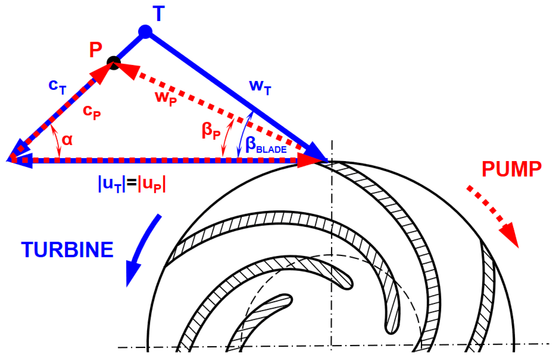
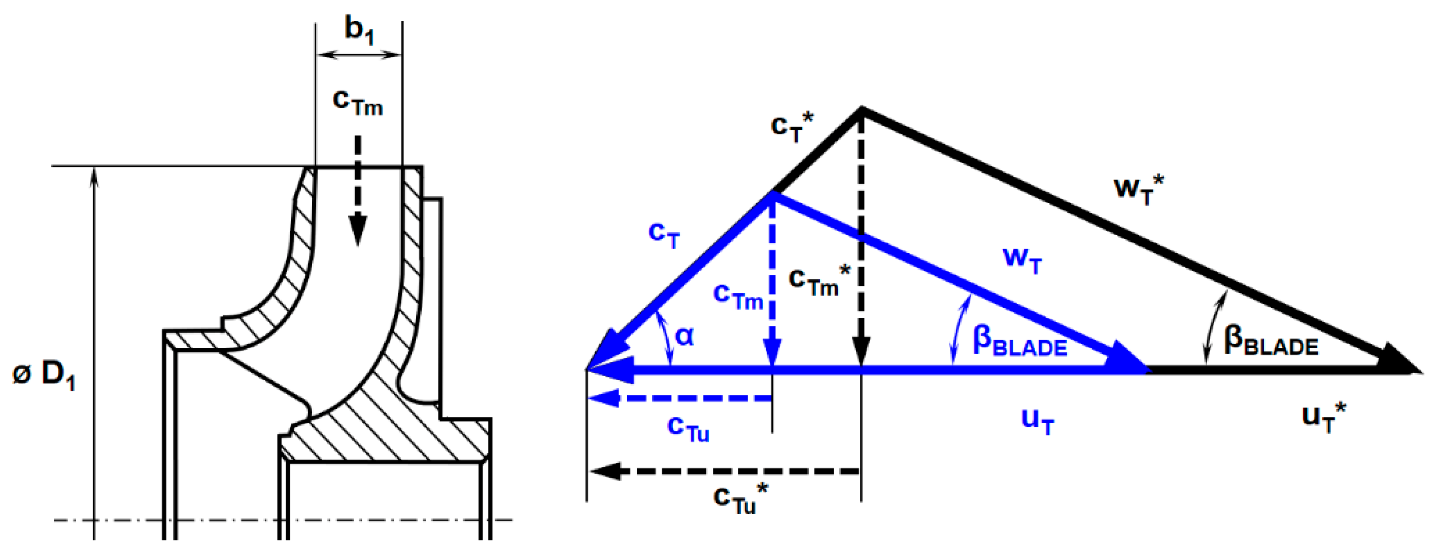
Parameters of Hydrodynamic Pumps in Turbine Operation

When comparing the pump and turbine operation, the optimal parameters differ. For turbine pump operation, the same circumferential velocity |u_P| = |u_T|, or the same shaft speed |N_P| = |N_T|, for pump operation is usually required. It is because of the use of synchronous motors, which can be operated in generator mode, and also because the production of electric power must respect the frequency of the grid. The kinematic conditions in the impeller during pump and turbine operation are shown by the velocity triangles in Figure 1. The dashed red lines represent the velocity triangle for pump mode, and the blue lines show the velocity triangle for reversed turbine mode. Vectors u_P and u_T represent circumferential blade velocity in the pump and turbine modes, respectively. Vectors c_P and c_T are the absolute velocities of the fluid and vectors w_P and w_T are the relative velocities of the fluid (relating to blade rotation) in pump and/or turbine mode.

Due to the diffuser flow of fluid through the impeller during pump operation, the fluid flow is less curved than the angle of the impeller blades at the outlet of the impeller (β_P < β_BLADE), so the velocity triangle meets at point P. In the case of turbine operation, assuming a shock-free flow, the fluid must flow into the impeller at an identical angle to the angle of the impeller blade (β_P = β_BLADE). As indicated by Capurso et al. [15], this difference leads to an increase in the absolute tangential velocity component and, therefore, to a reduction in the work extracted by the runner. To avoid the shock of the fluid entering the impeller, the vectors of the velocity triangle of the turbine operation must be joined at point T. A solution comes from a presumption presented by Bláha et al.: Since the height of the velocity triangles is proportional to the flow (Q), and the absolute velocity of the fluid (c) is the total head (H_T), the main parameters of the optimum pump turbine operation are as follows: Q_T > Q_P, H_T > H_P [16].

The conversion relationships between pump and turbine modes, i.e., between Q_P and Q_T or between H_P and H_T, vary according to the authors. An overview of the most cited methods is presented in

Table 1. Conversions according to various authors.

Author, Source	Head Ratio HT/HP	Flow Rate Ratio QT/QP	Note
Stepanoff, [18]	$\frac{1}{{\eta }_P}$	$\frac{1}{\sqrt{{\eta }_P}}$	Accurate for Ns = 40÷60
Childs, [19]	$\frac{1}{{\eta }_P}$	$\frac{1}{{\eta }_P}$	-
Hancock, [20]	$\frac{1}{{\eta }_T}$	$\frac{1}{{\eta }_T}$	-
Grover, [21]	$2.693-0.0229N_{sT}$	$2.379-0.0264N_{sT}$	Applied for Ns = 10÷50
Hergt, [22]	$1.3-\frac{6}{N_{qT}-3}$	$1.3-\frac{1.6}{N_{qT}-5}$	-
Sharma, [23]	$\frac{1}{{\eta }_P{}^{1.2}}$	$\frac{1}{{\eta }_P{}^{0.8}}$	Accurate for Ns = 40÷60
Schmiedl, [24]	$-1.4+\frac{2.5}{{\eta }_P}$	$-1.5+\frac{2.4}{{\eta }_P{}^2}$	-
Alatorre-Frenk, [25]	$\frac{1}{0.85{\eta }_P{}^5+0.385}$	$\frac{0.85{\eta }_P{}^5+0.385}{2{\eta }_P{}^{9.5}+0.205}$	-
Güllich, [26]	$\frac{2.4}{{\eta }_P{}^2}-1.5$	$\frac{2.5}{{\eta }_P}-1.4$	Volute casing Nq = 25÷220

. A detailed comparison between the results of individual conversion methods and reality is described in [17].

As mentioned by Stefanizzi et al., these methods are quite comprehensive, but it is difficult to apply them in practice, because they require very detailed geometric information, which is sometimes available only to the manufacturers [27]. As indicated, many researchers have therefore used different experimental techniques to predict PAT performance from pump characteristics. Kramer et al. concluded their study by saying that experimental investigations are still indispensable when an exact knowledge of turbine characteristics is required [28]. This issue is also addressed by Frosina et al. [29] who proved by experimental verification that some methods (e.g., Childs’ method) differ significantly from reality, while others (e.g., Stepanoff’s method) show small relative differences.

Correctly designed conversion relationships ensure maximum machine operation efficiency but only with nominal parameters. The conversion relationships presented in Table 1 assume constant operating parameters of total head, flow rate, and, especially, efficiency. However, in actual operation, the Q_T flow rate and the H_T gradient change, as does the shape of the velocity triangle. Thus, the vectors of individual velocities do not form a closed triangle. This also indicates a speed shock, resulting in a reduction in efficiency. For conventional turbines, this can be avoided by changing the geometry of the flow parts by turning the guide blades or impeller blades. However, pumps in turbine mode do not have blade control in the vast majority of cases. The solution can only be sought in the change of circumferential velocity, i.e., the shaft speed. This can be done by implementing gears or frequency inverters. In this way, the magnitude of the vectors changes, but the geometric similarity of the velocity triangles remains unchanged (α = constant, β_BLADE = constant). An explanation is presented in Figure 2. The vectors c_Tm and c_Tu are projections of absolute velocity in meridional and tangential directions, respectively, corresponding to nominal parameters. After changing the parameters (increasing flow rate and total head), the corresponding vectors are marked c_Tm* and c_Tu*. If the geometrical similarity of the triangles is maintained, speed shock does not occur, and the efficiency of the machine is not reduced.

3. Conversion Relationships of Hydraulic Machine Parameters

Based on the above assumption of the geometric similarity between the velocity triangles, a change in the operating parameters of PAT can be calculated according to Melichar [30]. The flow of the fluid through the inlet of the impeller at the nominal parameters Q_T (see Figure 2, the blue triangle) and at the changed parameters Q_T* (see Figure 2, the black triangle) comes from the following continuity equations:

$$Q_T=c_{Tm}·S_1=c_{Tm}·\pi ·D_1·b_1$$

(1)

and

$$Q_T^{*}=c_{Tm}^{*}·S_1=c_{Tm}^{*}·\pi ·D_1·b_1$$

(2)

By dividing Equations (1) and (2) Q_T*/Q_T, provided that π, D₁, b₁ = constant, we get the following:

$$Q_T^{*}=Q_T·\frac{c_{Tm}^{*}}{c_{Tm}}$$

(3)

The meridional component of the absolute velocity c_Tm is proportional to absolute velocity c, which is given by the total head of the turbine. The same applies for $c_{Tm}^{*}$ with changed parameters. The absolute speed also determines the turbine impeller speed or shaft speed N_T:

$$c_{Tm}\approx c_T\approx N_T$$

(4)

and

$$c_{Tm}^{*}\approx c_T^{*}\approx N_T^{*}$$

(5)

From using the relationships presented in Equations (4) and (5) in Equation (3), we get the following:

$$Q_T^{*}=Q_T·\frac{N_T^{*}}{N_T}$$

(6)

It follows from Equation (6) that if the flow rate changes from nominal value Q_T to value Q_T*, it is necessary to change the shaft speed in order to maintain the geometric similarity of the velocity triangle to the following:

$$N_T^{*}=N_T·\frac{Q_T^{*}}{Q_T}$$

(7)

The total head, or the specific energy, at the turbine nominal parameters Y_T and the changed parameters Y_T* is expressed by the Euler equation, assuming a vortex-free fluid output from the impeller.

$$Y_T=u_T·c_{Tu}$$

(8)

and

$$Y_T^{*}=u_T^{*}·c_{Tu}^{*}$$

(9)

The circumferential velocity of the impeller at the inlet u_T, at a constant diameter D₁, is given only by the shaft speed N_T:

$$u_T=\pi ·D_1·N_T$$

(10)

and

$$u_T^{*}=\pi ·D_1·N_T^{*}$$

(11)

Analogously to Equations (4) and (5), the magnitude of the projection of the absolute velocity c_Tu is given by the magnitude of absolute velocity or by the shaft speed.

$$c_{Tu}\approx c_T\approx N_T$$

(12)

and

$$c_{Tu}^{*}\approx c_T^{*}\approx N_T^{*}$$

(13)

By substituting the relationships in Equations (10), (11) and (12), (13) into Equations (8) and (9), presuming D₁ = constant, and by dividing Equations (8) and (9) Y_T*/Y_T, we come to the following:

$$Y_T^{*}=Y_T·{\left(\frac{N_T^{*}}{N_T}\right)}^2$$

(14)

When changing the specific energy, or the total head, it is necessary to change the shaft speed to maintain the optimum efficiency as follows:

$$N_T^{*}=N_T·\sqrt{\frac{H_T^{*}}{H_T}}$$

(15)

The power output of the turbine operating with a fluid of density ρ at nominal parameters P_T and changed parameters P_T* is given by the following:

$$P_T=Q_T·\mathsf{\rho }·{\mathrm{Y}}_T$$

(16)

and

$$P_T^{*}=Q_T^{*}·\mathsf{\rho }·Y_T^{*}$$

(17)

By dividing Equations (16) and (17) P_T^*/P_T, and by subsequent modification, we get a relationship for power output at changed total head, flow rate and shaft speed:

$$P_T^{*}=P_T·{\left(\frac{N_T^{*}}{N_T}\right)}^3$$

(18)

The above procedures can also be used to determine the torque:

$$M_T^{*}=M_T·{\left(\frac{N_T^{*}}{N_T}\right)}^2$$

(19)

The characteristics of the turbine at the changing parameters are given by merging the affine relationships of Equations (6) and (14) that result in the following:

$$\frac{Y_T^{*}}{Y_T}={\left(\frac{Q_T^{*}}{Q_T}\right)}^2$$

(20)

By separating Y*, we get an equation of so-called affine parabola with the vertex at the beginning of the coordinates Y_T*–Q_T*.

$$Y_T^{*}=\frac{Y_T}{Q_T^2}·{\left(Q_T^{*}\right)}^2=k·{\left(Q_T^{*}\right)}^2$$

(21)

The affine parabola links together points corresponding to maximum efficiency. The optimum operating point of the pump in turbine mode must lie on or very near to the affine parabola. The position of the working point is controlled either by throttling at the end of the pressure line or in the bypass of the pump or by changing the shaft speed by means of a gear or frequency inverter. The speed change follows the maximum efficiency curve or the constant flow requirement, e.g., in order to maintain sanitary flow in the riverbed if the pump is placed at the base outflow of a water reservoir as indicated by Melichar et al. [31].

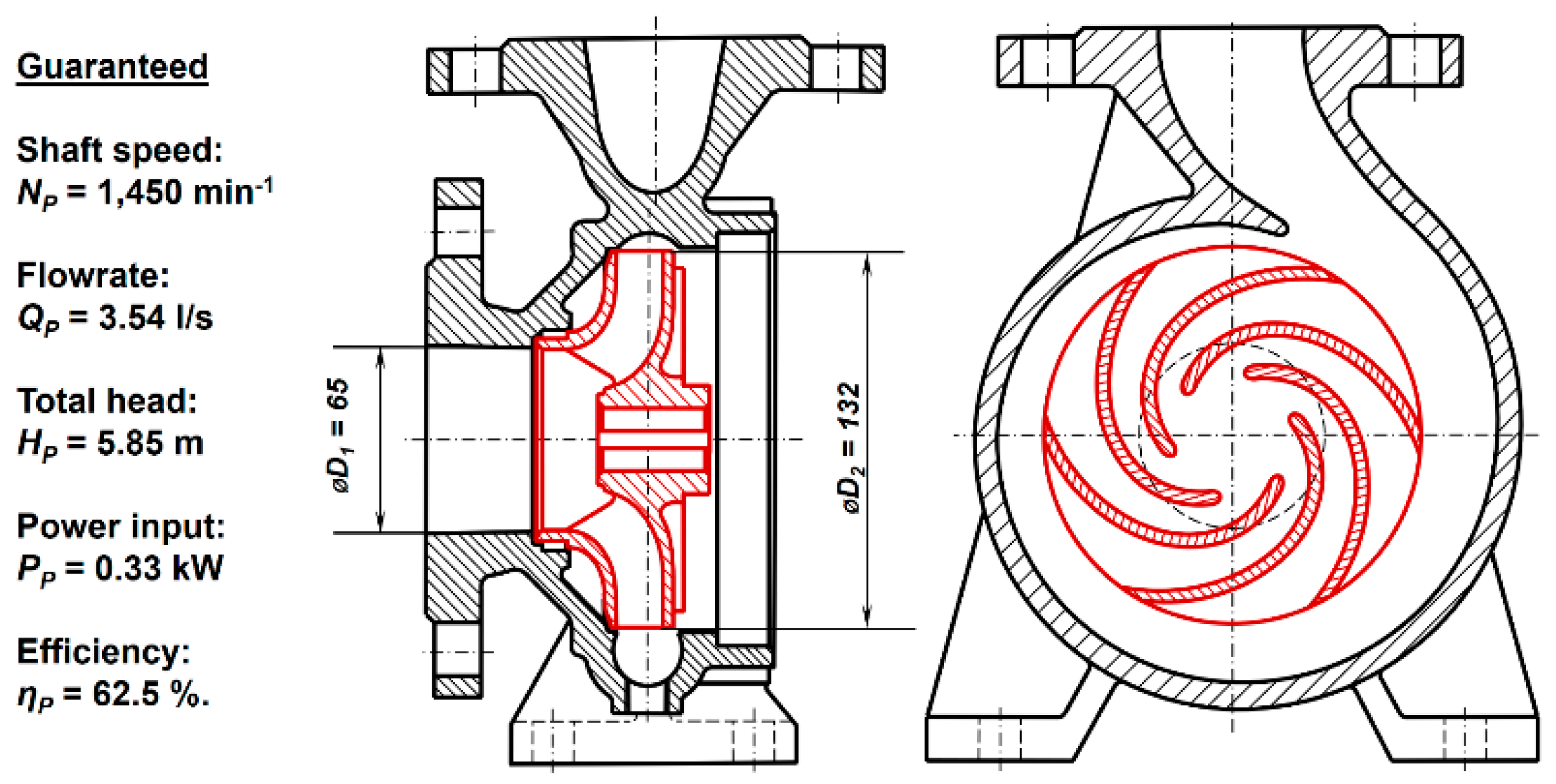
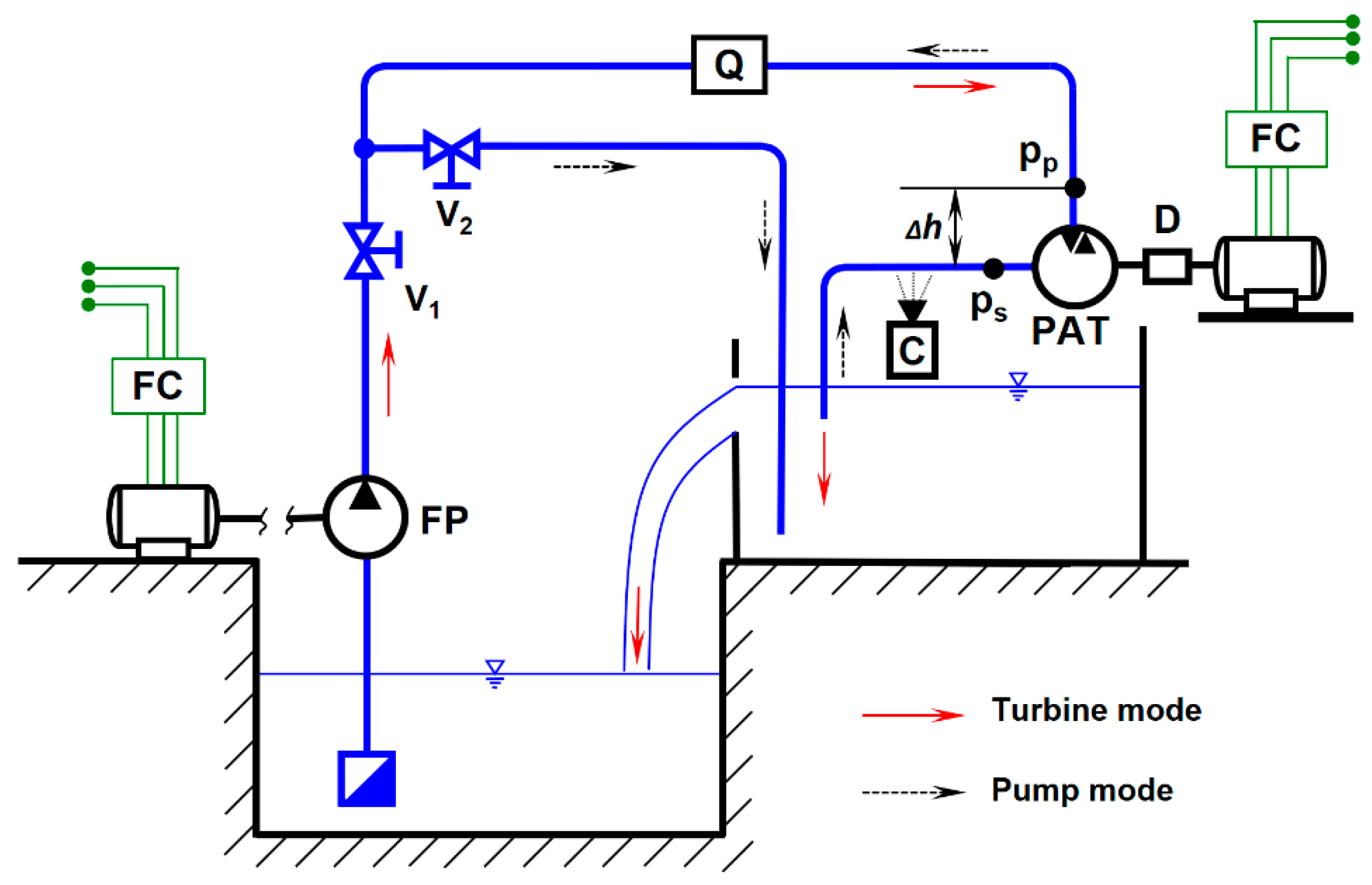
4. Experimental Verification of Model Calculations of Turbine Operation

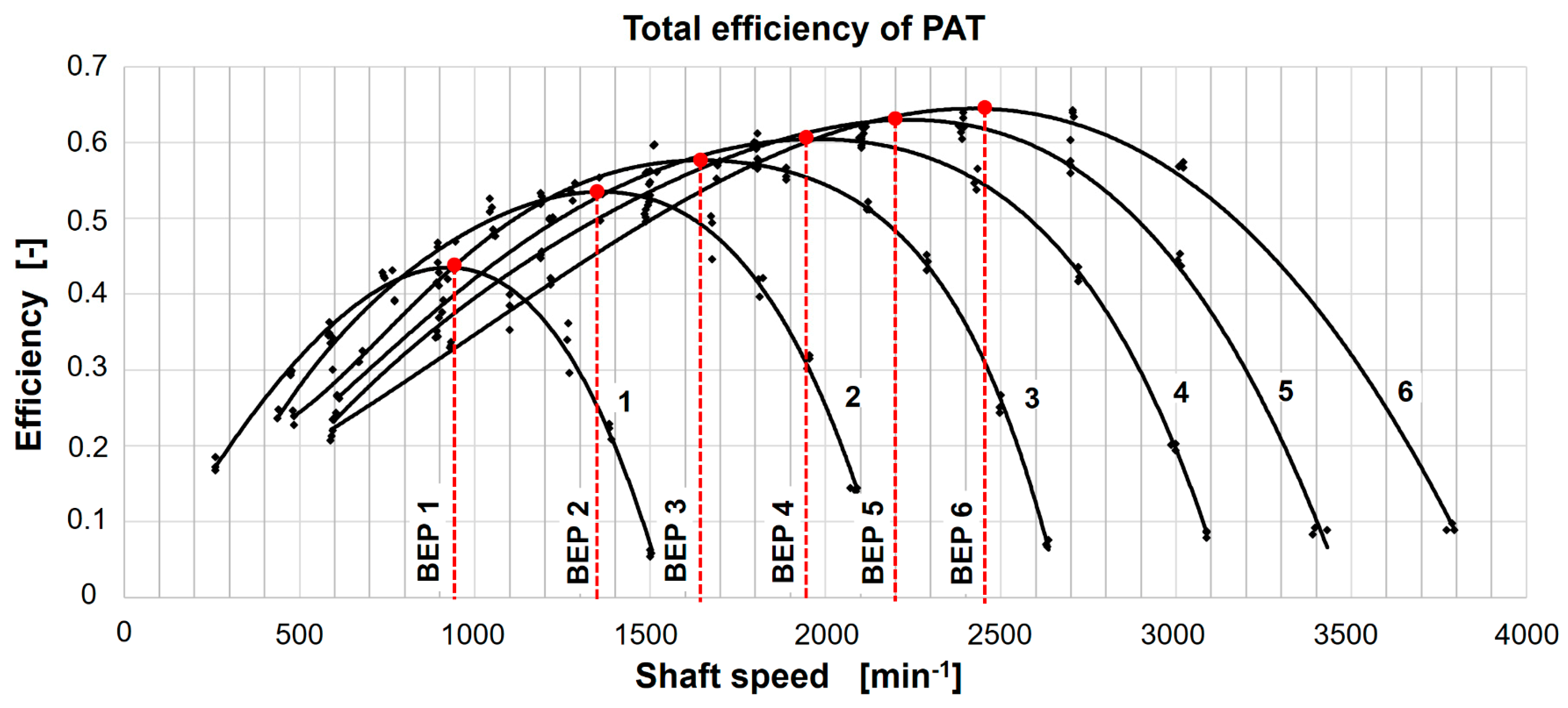
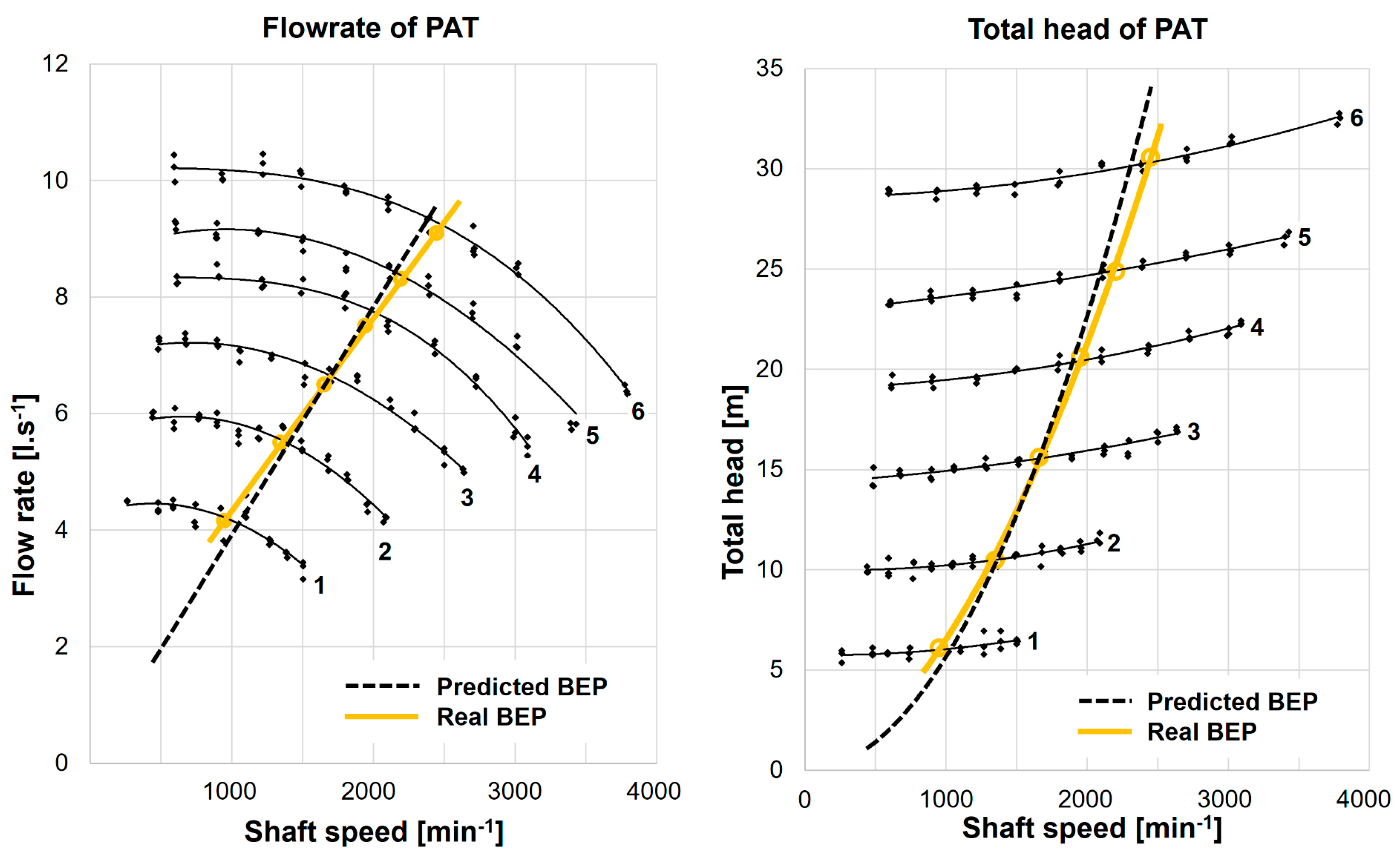
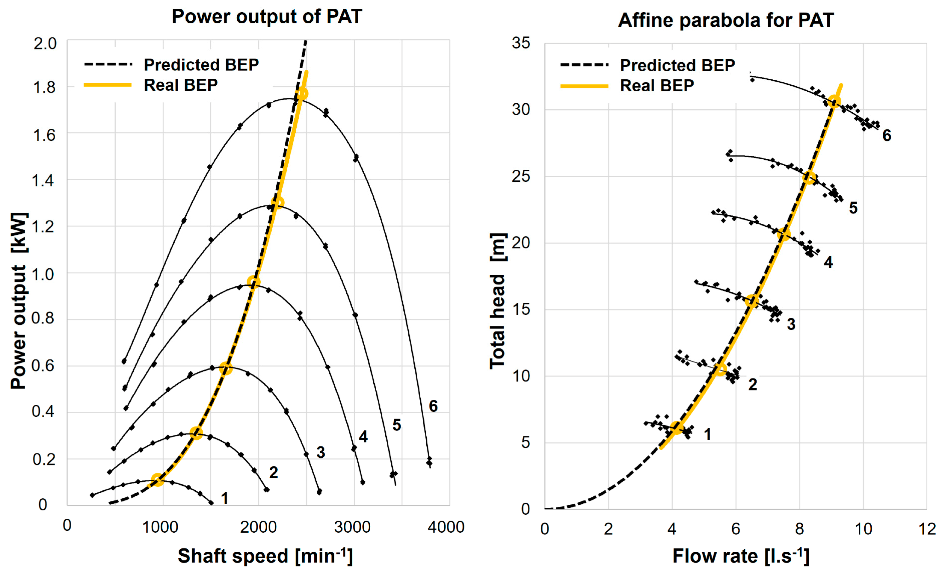
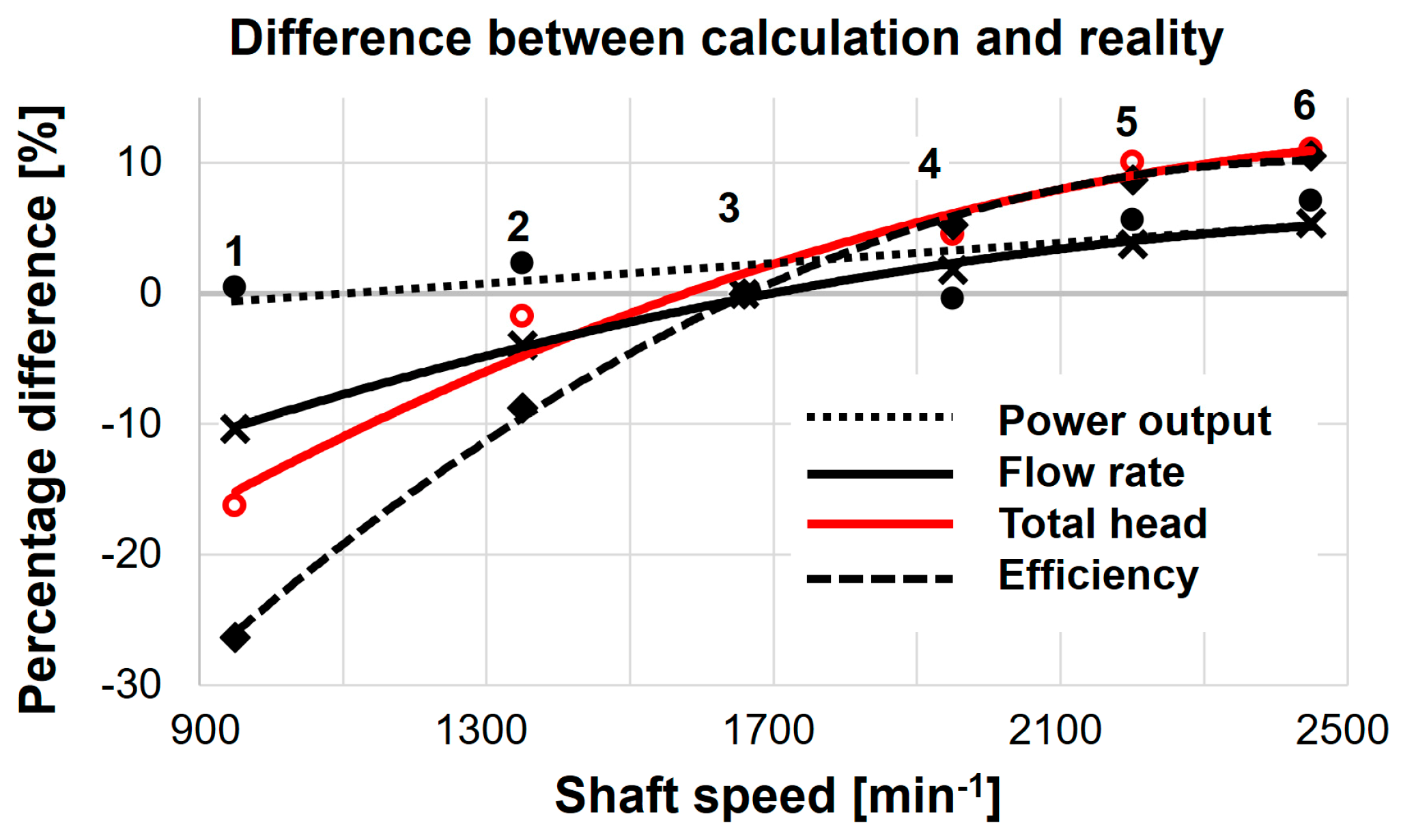
The abovementioned methodology was verified at the author’s workplace on a radial single stage centrifugal META series pump, manufactured in the Czech Republic by ISH Pumps, Olomouc. The pump’s scheme and parameters in pump mode, as provided by the manufacturer, are presented in Figure 3.

Verification tests were conducted on a hydraulic circuit in the fluid mechanics laboratory at the faculty of engineering, Czech University of Life Sciences, Prague. The circuit diagram is shown in Figure 4.

The testing circuit consisted of a set of two reservoirs with pipes and control and measuring elements. With this setting, the tested PAT was measured in turbine mode. By closing valve V₂, the water flowed in the direction of the dashed arrows, while the feeding pump (FP) created the hydropower potential for the turbine. The dynamometer (D) with momentum sensor Magtrol TMB 307/41 (accuracy 0.1%) allowed continuous regulation of shaft speed via the frequency inverter LSLV0055s100-4EOFNS. This device enabled operation in motor and braking modes. The water flow was measured using an electromagnetic flowmeter (Q) SITRANS F M MAG 5100 W (accuracy 0.5%). Pressures at p_p and p_s were measured by pressure sensor HEIM 3340 (accuracy 0.5%) installed according to first class accuracy requirements [32].

5. Results

The aim of the experimental part of this study was to verify the behavior of PAT in general piping systems, allowing the generation of energy from a flowing liquid. The main experiment consisted of measuring performance parameters of PATs at six basic hydropower potentials (modes) that simulated changing pipeline system parameters. Constant hydropower potential was ensured by the constant speed of the feeding pump (FP), which means that six measurements were taken at six constant speed settings of the FP. During the measurements, PAT was gradually loaded from idle speed up to N_T ≈ 500 min⁻¹ in each mode. The performance characteristics were determinedfrom the measured values. Figure 5 presents the dependence of efficiency on shaft speed. Based on this dependence, the BEP was determined for each mode.

The following parameters corresponding to optimum operation at the BEP were determined from other characteristics, i.e., flow rate, total head, and power output. An overview of all monitored parameters is presented in

Table 2. Performance parameters of tested PAT at BEP.

Hydropower Potential (Mode)	1	2	3	4	5	6
Total efficiency: ηT [%]	44 ± 1.9	53 ± 1.6	57 ± 0.6	61 ± 0.7	62 ± 0.7	63 ± 0.7
Shaft speed: NT [min−1]	950	1350	1650	1950	2200	2450
Flow rate: QP [l.s−1]	4.1 ± 0.16	5.7 ± 0.12	6.6 ± 0.07	7.5 ± 0.05	8.5 ± 0.07	9.3 ± 0.08
Total head: HT [m]	6.0 ± 0.25	10.5 ± 0.31	16.0 ± 0.17	20.7 ± 0.23	25.0 ± 0.30	30.2 ± 0.31
Power output: PT [W]	107 ± 0.9	306 ± 0.8	588 ± 1.0	926 ± 1.5	1282 ± 2.3	1737 ± 4.0

.

In order to verify the applicability of the predictive relationships in Equations (6), (14), (15), and (18) and in the affine parabola in Equation (21), other necessary characteristics were determined from the measured values. Figure 6 presents the effects of flow rate and total head dependence on shaft speed. Values for the BEP (yellow curves) from Table 2 are marked here, as well as curves from the predictive calculations (dashed lines) according to Equations (6) and (15). The parameters measured in mode 3 were used as input values for the predictive calculations.

The characteristics presented in Figure 7 were generated in a similar way. These are the dependences of power output on speed and the affine parabola, including the measured values (yellow curve) and the calculated values (dashed line) for the BEP.

From the achieved results, the relative deviations of the monitored output parameters were subsequently determined:

$$\mathsf{\Delta }A=100·\frac{A_C-A_R}{A_R}$$

(22)

where A_C is the calculated value and A_R is the measured value. To make the overview of the deviation size and trend clearer, the individual parameters were compared to speed and presented in Figure 8.

The graph in Figure 8 summarizes the final results of the study and serves to compare the experimentally measured values with the results of the calculated prediction of flow rate, Equation (6); total head, Equation (15); and power output, Equation (18) in relation to shaft speed.

6. Discussion

Based on the comparison of the results from Figure 8, the following can be stated: The deviation of the values in mode 3 was zero, because this mode was defined as the base reference mode. The deviation of the power output calculation at varying potentials was minimal (6% at the most), so the conversion ratio in Equation (18) can be used in practice. Similarly, the relationship of the affine parabola in Equation (21) can be used to determine the optimum total head and flow rate to ensure maximum PAT operation efficiency.

The deviations of other variables (the flow rate and total head dependence on shaft speed) gradually increased with increasing distance from reference mode 3, more so as the difference between the reference and the actual value of efficiency increased (from point 3 to the left). The cause of efficiency reduction can be found in the speed shock of the fluid at the impeller inlet. The absolute velocity c decreases at a lower hydropower potential; thus, the velocity triangle does not close at point T. This results in a speed shock and hydraulic loss as described in Figure 1.

On the other hand, where efficiency changed only a little, the other parameters changed in a similar way (from point 3 to the right). To put it simply, the deviation from the predicted efficiency was the cause of the deviation of the other parameters. However, if there is a stable potential provided during the PAT operation, all the above calculation methods are reliably applicable.

7. Conclusions

The use of PATs is one of the possibilities for the provision of cost-effective solutions for energy savings in WDN systems or for power generation in small hydropower plants. Economically advantageous solutions require technically optimized equipment for a wide range of operating parameters. Due to the limited possibility of PAT control on the input hydraulic parameters, it is necessary to focus the optimization on the output parameters, e.g., by way of speed control using frequency inverters. These would allow a flexible response for changing PAT operating parameters and provide the maximum benefit for its user. This article described the influence of the change of hydropower potential on PAT operation and compared the experimental results with the model of theory of physical similarity. The model used did not include a change in efficiency similar to models of other authors who also did not consider varying efficiency. However, the results of the experimental verification proved that neglecting the variability of efficiency leads to an incorrect setting of the optimum operational parameters. This applies particularly to the flow rate and the total head dependence on shaft speed, which are the most important relationships when optimizing PAT operation.

The main purpose of the article is to confirm the influence of changing hydropower potential on changes in efficiency. In order to use PAT efficiently under the conditions of variable potential, it is necessary to focus on this issue more deeply and to theoretically describe and include the changes in efficiency in the conversion relationships in order to ensure the optimum operational parameters. A more detailed analysis of this issue will be the subject of further research.

References

1. Giosio, D.R.; Henderson, A.D.; Walker, J.M.; Brandner, P.A.; Sargison, J.E.; Gautam, P. Design and performance evaluation of a pump-as-turbine micro-hydro test facility with incorporated inlet flow control. Renew. Energy 2015, 78, 1–6. [Google Scholar] [CrossRef]
2. Williams, A.A. Pumps as turbines for low cost micro hydro power. Renew. Energy 1996, 9, 1227–1234. [Google Scholar] [CrossRef]
3. Pugliese, F.; De Paola, F.; Fontana, N.; Giugni, M.; Marini, G. Experimental characterization of two pumps as turbines for hydropower generation. Renew. Energy 2016, 99, 180–187. [Google Scholar] [CrossRef]
4. Jain, S.V.; Patel, R.N. Investigations on pump running in turbine mode: A review of the state-of-the-art. Renew. Sustain. Energy Rev. 2014, 30, 841–868. [Google Scholar] [CrossRef]
5. Carravetta, A.; del Giudice, G.; Fecarotta, O.; Ramos, H.M. PAT design strategy for energy recovery in water distribution networks by electrical regulation. Energies 2013, 6, 411–424. [Google Scholar] [CrossRef]
6. Fontana, N.; Giugni, M.; Portolano, D. Losses reduction and energy production in water-distribution networks. J. Water Res. Plan. 2012, 138, 237–244. [Google Scholar] [CrossRef]
7. Førsund, F.R. Pumped-storage hydroelectricity. In Hydropower Economics; International Series in Operations Research & Management Science: Springer, Boston, MA, USA, 2015; Volume 127. [Google Scholar]
8. Barbarelli, S.; Amelio, M.; Florio, G. Experimental activity at test rig validating correlations to select pumps running as turbines in microhydro plants. Energy Convers. Manag. 2017, 149, 781–797. [Google Scholar] [CrossRef]
9. Polák, M. Experimental evaluation of hydraulic design modifications of radial centrifugal pumps. Agron. Res. 2017, 15, 1189–1197. [Google Scholar]
10. Singh, P. Optimization of the Internal Hydraulics and of System Design for Pumps as Turbines with Field Implementation and Evaluation. Ph.D. Thesis, University of Karlsruhe, Karlsruhe, Germany, 2005. [Google Scholar]
11. Singh, P.; Nestmann, F. Internal hydraulic analysis of impeller rounding in centrifugal pumps as turbines. Exp. Therm. Fluid Sci. 2011, 35, 121–134. [Google Scholar] [CrossRef]
12. Derakhshan, S.; Mohmmadi, B.; Nourbakhsh, A. Efficiency improvement of centrifugal reverse pumps. J. Fluids Eng. 2009, 131, 021103. [Google Scholar] [CrossRef]
13. Jain Sanjay, V.; Swarnkar Abhishek Motwani Karan, H.; Patel Rajesh, N. Effects of impeller diameter and rotational speed on performance of pump running in turbine mode. Energy Convers. Manag. 2015, 89, 808–824. [Google Scholar] [CrossRef]
14. Venturini, M.; Alvisi, S.; Simani, S.; Manservigi, L. Energy production by means of pumps as turbines in water distribution networks. Energies 2017, 10, 1666. [Google Scholar] [CrossRef]
15. Capurso, T.; Stefanizzi, M.; Torresi, M.; Pascazio, G.; Caramia, G.; Camporeale, S.; Fortunato, B.; Bergamini, L. How to improve the performance prediction of a pump as turbine by considering the slip phenomenon. Proceedings 2018, 2, 683. [Google Scholar] [CrossRef]
16. Bláha, J.; Melichar, J.; Mosler, P. Contribution to the use of hydrodynamic pumps as turbines. Energetika 2012, 5, 1–5. (In Czech) [Google Scholar]
17. Polák, M. Determination of conversion relations for the use of small hydrodynamic pumps in reverse turbine operation. Agron. Res. 2018, 16, 1200–1208. [Google Scholar]
18. Stepanoff, A.J. Centrifugal and Axial Flow Pumps, Design and Applications; John Willy and Sons, Inc.: New York, NY, USA, 1957; 462p. [Google Scholar]
19. Childs, S.M. Convert pumps to turbines and recover HP. Hydro Carbon Process. Petrol. Refin. 1962, 41, 173–174. [Google Scholar]
20. Hancock, J.W. Centrifugal pump or water turbine. Pipe Line News 1963, 6, 25–27. [Google Scholar]
21. Grover, K.M. Conversion of Pumps to Turbines; GSA Inter Corp.: Katonah, NY, USA, 1980; pp. 125–138. [Google Scholar]
22. Lewinsky-Keslitz, H.P. Pumpen als Turbinen fur Kleinkraftwerke. Wasserwirtschaft 1987, 77, 531–537. [Google Scholar]
23. Sharma, K. Small Hydroelectric Project-Use of Centrifugal Pumps as Turbines; Technical Report; Kirloskar Electric Co.: Bangalore, India, 1985; pp. 14–26. [Google Scholar]
24. Schmiedl, E. Serien-Kreiselpumpen im Turbinenbetrieb; Pumpentagung: Karlsruhe, Germany, 1988. [Google Scholar]
25. Alatorre-Frenk, C. Cost Minimization in Micro Hydro Systems Using Pumps-As-Turbines. Ph.D. Thesis, University of Warwick, Warwick, UK, 1994. [Google Scholar]
26. Gülich, J.F. Centrifugal Pumps, 3rd ed.; Springer: Berlin, Germany, 2008; 1116p, ISBN 978-3-642-40113-8. [Google Scholar]
27. Stefanizzi, M.; Torresi, M.; Fortunato, B.; Camporeale, S.M. Experimental investigation and performance prediction modeling of a single stage centrifugal pump operating as turbine. Energy Procedia 2017, 126, 589–596. [Google Scholar] [CrossRef]
28. Kramer, M.; Terheiden, K.; Wieprecht, S. Pumps as turbines for efficient energy recovery in water supply networks. Renew. Energy 2018, 122, 17–25. [Google Scholar] [CrossRef] [Green Version]
29. Frosina, E.; Buono, D.; Senatore, A. A performance prediction method for pumps as turbines (PAT) using a computational fluid dynamics (CFD) modeling approach. Energies 2017, 10, 103. [Google Scholar] [CrossRef]
30. Melichar, J.; Bláha, J. Problems of Contemporary Pumping Technology, Selected Parts; ČVUT: Prague, Czech Republic, 2007; p. 265. (In Czech) [Google Scholar]
31. Melichar, J.; Vojtek, J.; Bláha, J. Small Hydro Turbines, Construction and Operation; ČVUT: Prague, Czech Republic, 1998; p. 296. (In Czech) [Google Scholar]
32. European Committee for Standardization. Rotodynamic Pumps—Hydraulic Performance Acceptance Tests—Grades 1, 2 and 3; ČSN EN ISO 9906; European Committee for Standardization: Brussels, Belgium, 2013. (In Czech) [Google Scholar]
Figure 1. Kinematic conditions during pump and turbine operation.
Energies 12 02103 g001
Figure 2. The change of kinematic conditions during turbine operation.
Energies 12 02103 g002
Figure 3. Pump used for experimental tests.
Energies 12 02103 g003
Figure 4. Hydraulic circuit scheme for testing turbines/pumps; Q, flowmeter; FP, feed pump; PAT, pump as turbine; V1, and V2, control valves; D, dynamometer; FC, frequency inverter; C, camcoder.
Energies 12 02103 g004
Figure 5. Courses of efficiency in modes 1–6 highlighting the optimum best efficiency point (BEP).
Energies 12 02103 g005
Figure 6. Predictive calculations of flow rate and total head versus reality.
Energies 12 02103 g006
Figure 7. Predictive calculations of power output and affine parabola versus reality.
Energies 12 02103 g007
Figure 8. Comparison of predictive calculations with reality.
Energies 12 02103 g008