Article

Uncertainy’s Indices Assessment for Calibrated Energy Models

by
Vicente Gutiérrez González
1,*,
Lissette Álvarez Colmenares
2,
Jesús Fernando López Fidalgo
2,
Germán Ramos Ruiz
1 and
Carlos Fernández Bandera
1
1
School of Architecture, University of Navarra, 31009 Pamplona, Spain
2
ICS Statistical Unit, University of Navarra, 31009 Pamplona, Spain
*
Author to whom correspondence should be addressed.
Energies 2019, 12(11), 2096; https://doi.org/10.3390/en12112096
Submission received: 5 April 2019 / Revised: 22 May 2019 / Accepted: 27 May 2019 / Published: 31 May 2019

Abstract

:
Building Energy Models (BEMs) are a key element of the Energy Performance of Buildings Directive (EPBD), and they are at the basis of Energy Performance Certificates (EPCs). The main goal of BEMs is to provide information for building stakeholders; they can be a powerful market tool to increase demand for energy efficiency solutions in buildings without affecting the comfort of users, as well as providing other benefits. The next generation of BEMs should value buildings in a holistic and cost-effective manner across several complementary dimensions: envelope performances, system performances, and controlling the ability of buildings to offer flexible services to the grid by optimizing energy consumption, distributed generation, and storage. SABINA is a European project that aims to look for flexibility to the grid, targeting the most economic source possible: existing thermal inertia in buildings. In doing so, SABINA works with a new generation of BEMs that tend to mimic the thermal behavior of real buildings and therefore requires an accurate methodology to choose the model that complies with the requirements of the system. This paper details our novel extensive research on which statistical indices should be chosen in order to identify the best model offered by the calibration process developed by Fernandez et al. in a previous paper and therefore is a continuation of that work.

1. Introduction and Motivation for the Work

BEMs are key elements of the Energy Performance of Buildings Directive, and they are at the basis of Energy Performance Certificates (EPCs) and assessment. Assessment and certification processes should be user-friendly, cost-effective, and more reliable in order to instill trust in investors in the energy efficiency sector [1]. Therefore, the next generation of EPCs will need to fulfill these requirements, as well as the next generation of BEMs. Until now, EPCs have been based on two concepts [2]: standard energy rating and measured energy rating. In the former, the energy consumed by a building is calculated through an energy model (law-driven models, Option D of the International Performance Measurement and Verification Protocol (IPMVP)) [3], and in the latter, the energy is measured through meters and sensors installed in the building (data-driven models, Option C of the IPMVP).
In a previous paper written by some of the authors [4], it was explained in detail how this new generation of BEMs should be produced and that the new technique is able to merge the law-driven models [5] and the data-driven models [6,7,8,9], resulting in “law-data-driven models”. In summary, the concept uses well-known software such as EnergyPlus [10] to combine the model based on as-built parameters with the model based on parameters estimated using measurements of the system and, through a calibration process, producing the new technique. This technique has produced very good results and is based on the use of measured temperature from the real building as part of the energy balance of the BEM, following the idea that Sonderegger postulated in 1977: “Instead of telling the computer how the building is built and asking it for the indoor temperature, one tells the computer the measured indoor temperature and asks it for the building parameters” [11].
SABINA is a project that is looking for services on the grid based on the “demand response” concept [12] and the idea of increasing the amount of renewable energy consumed locally by buildings. To reach the EU’s long-term objectives for reducing greenhouse gas emissions, this share should reach more than 30% in 2030, and almost 50% in some scenarios in 2050 [13]; new management systems are thus required. What is most needed is additional flexibility in the system. SABINA targets the most economic source possible: existing thermal inertia in buildings [14]. This goal requires models that capture the thermal dynamics of the building, and the Zero Energy Calibration (ZEC) methodology has been chosen to select those kinds of models [4]. The usefulness of a model depends on the accuracy and reliability of its output, but all models are imperfect abstractions of reality, because there is imprecision and uncertainty associated with any model.
Currently, there is the protocol IPMVP [3], and two guidelines: FEMP [15] and ASHRAE [16], which offer a set of error indices ( C V ( R M S E ) , N M B E , and R 2 ) to evaluate the quality of the calibrated models considering the monthly and hourly energy consumption (simulated vs. real). Other methodologies use indoor air temperature (simulated vs. real) to calibrate the building models with the same indices [4,17,18,19,20]. When doing so, it is not clear if these indices, which were selected for energy evaluation, will have a good performance for temperature. In this paper, a large number of error indices have been analyzed with the aim of selecting the best ones to choose the model that represents the real building indoor air temperature. This new evaluation methodology has been tested and verified in different building models: the “Amigos” [4], “Humanities” [21], and “The School of Architecture” [22] at the Pamplona Campus of the University of Navarre. In this paper, the office building of the School of Architecture has been used, as it is explained in the following sections.

Summary of the ZEC Methodology

The Zero Energy Calibration (ZEC) is a methodology for building envelope calibration. The ZEC principle is based on the idea that when introducing the free oscillation temperature of a building in the model, as a dynamic set-point, the energy consumed by the HVAC equipment in that period should be zero. If this is not the case, the reason should be the wrong configuration of the building parameters, and the algorithm (genetic algorithm) will look for a new vector of envelope parameters that will produce a lower energy consumption (heating plus cooling). The process finishes when the energy (the objective function) cannot be reduced further and the model envelope is calibrated.
In most automatic calibration techniques [23,24], the simulation data are used at the end of the process to be compared with the measured data, and the goal is to minimize an error value in what is known as uncertainty analysis. In such cases, the statistical indices ( C V ( R M S E ) , N M B E , and R 2 ) are the objective functions that will guide the algorithm in the search for the calibrated model [25,26,27].
The main ways of calibration do not allow entering into the calibration process as many measured data as necessary, and thus, the thermal characterization of the model will not be improved. In this methodology (ZEC), there is no restriction in the creation of thermal zones. The major simplification that ZEC offers is that there is no implementation of uncertainty analysis in coordination with the automatic calibration algorithm and the simulation program, which makes it simpler and therefore more accessible to all kinds of professionals with energy simulation skills, but without programing capabilities.
For this reason, the ZEC methodology is simple in execution. The algorithm used to perform the thermal zone energy balance in EnergyPlus is the Conduction Transfer Function (CTF), which offers a very fast and elegant solution to solve the Fourier differential equation and to find the temperature of the thermal zone. However, as explained in the EnergyPlus Engineering Reference, “conduction transfer function series become progressively more unstable as the time step decreases. This became a problem as investigations into short time step computational methods for the zone/system interactions progressed because, eventually, this instability caused the entire simulation to diverge” [28]. This divergence is translated into extra energy consumption that affects the objective function used by ZEC, a problem that has been well documented and evaluated by Wetter et al. [29]. The result of this extra energy consumption is that some models with slightly higher energy consumption have better uncertainty temperature results than the best models selected by the energy of the objective function. From a practical point of view, this means that the best model cannot be chosen directly from the results offered by the algorithm unless an uncertainty temperature analysis is subsequently performed, in the same way as other similar works [26,27,30,31].
Taking into account the indices’ combination proposed by ASHRAE ( C V ( R M S E ) , N M B E , and R 2 ) [16], the authors worked with a new statistical index that was called the Z E C _ I n d e x [4], which was the arithmetic sum of errors C V ( R M S E ) , N M B E , and ( 1 R 2 ) . The model with the lowest Z E C _ i n d e x was the one considered to have the best performance. As the indices’ combination proposed by ASHRAE ( C V ( R M S E ) , N M B E , and R 2 ) is based on energy uncertainty analysis and the new proposal is based on temperature uncertainty analysis, this paper intends to confirm if there is any other statistical index or combination of indices that can improve the selection of the best model.
The uncertainty analysis should classify the best models according to the capacity to reduce the error between real temperature inside the building and simulated temperature produced by the building model. From a practical point of view, a good correlation should be found between temperature and energy with respect to the selected temperature error (uncertainty index).
In order to check if a different index can choose a better model, a list of a number of error metrics that been studied in Section 2, classified into seven groups (bias error indices, uncertainty indices based on absolute deviations, uncertainty indices based on square deviations, goodness-of-fit metrics, efficiency criteria, indices for model discrimination, and proximity measures), according to the application or structure and the statistical methodology description used to select the metrics that identify the best-adjusted calibrated energy model. Section 3 outlines the cases of study and the description of the building used to check the methodology. Section 4 presents the performance of the metrics described in Section 2 over two case studies: a synthetic energy model and a real building model, each under the same conditions. The conclusions that we have reached in this paper and future research considerations are presented in Section 5.

2. List of a Number of Error Metrics

Having a “reasonable” idea of the quality of adjustment between real and simulated models is not hard [32], but evaluating the accuracy of a BEM or quantifying the quality of the adjustment is, actually, quite difficult, particularly when this quantification is used to identify the best adjusted model to the real building.
Different indices are used in diverse research branches to define an evaluation criterion for the accuracy of the energy model. For example, efficiency measures are used in hydrology [33,34]. In order to evaluate the performance of the model for energy saving in the Measurement and Verification process (M&V), Goodness-of-fit metrics are generally used [35]. Another measure, known as the uncertainty index, is used in an energy modeling context for the same purpose [36].
Each metric provides a different insight into the model’s performance, and therefore, there is no an ideal metric to identify the best-adjusted model. In fact, researchers suggest “to use the numerical comparison as well as graphical comparison when one decides the base model adequacy” [37]. In practice, several metrics are jointly evaluated and complemented by a graphical analysis (e.g., [38,39,40,41]).

2.1. Bias Error Indices

The range for all of these is the whole real line, and the optimal value must be zero (Table 1). The M&V methodology for energy calibrated models considers p = 1 for N M B E .

2.2. Uncertainty Indices Based on Absolute Deviations

These indices consider only the distance between values, omitting the direction of the differences and overcoming cancellation errors. They can take any positive value, and their optimal value is minimum (Table 2).

2.3. Uncertainty Indices Based on Square Deviations

In square deviation measures (Table 3), the M&V methodology for energy calibrated models considers p = 1 for C V ( R M S E ) .

2.4. Goodness-of-Fit Metrics

The uncertainty in energy calibrated models is directly related to their goodness-of-fit [42] and is the reason why they are the most popular measures to establish the fitness of a simulated model (Table 4). They measure the quality of the linear relationship between the simulated and observed data. This relationship may be quite strong, but with a substantial bias. Thus, these measures may be completed with the bias measures. It may be said that uncertainty can be assessed with a couple of measures, one of the goodness-of-fit and one of bias.

2.5. Efficiency Criteria

This indices are measures of how well a model simulation fits the real observations [43], and they are widely used, for instance, to evaluate the performance of hydrological models [33,34]. Most of the efficiency criteria include notions of distance and variance between real and simulated values in order to analyze the adjustment, both in terms of location and variability. Table 5 shows the indices considered here.

2.6. Indices for Model Discrimination

The Akaike Information Criterion ( A I C ) and Bayesian Information Criterion ( B I C ) are used for choosing among different models, as Table 6 indicates.

2.7. Proximity Measures

p f a c t o r (34) is the proportion of simulated values that are within a given band of the observed values and, therefore, takes values in [ 0 , 1 ] .
p f a c t o r = A n A = { y ^ i [ y i λ , y i + λ ] , i = 1 , , n }
If the simulated model represents exactly the behavior of the real model, p f a c t o r = 1 for small λ -wide uncertainty bounds, which is equivalent to obtaining 100% of observations within the uncertainty band [44]. Therefore, the model error could be referenced by ( 1 , p f a c t o r ). A perfect adjustment of models has a p f a c t o r equal to one.
This measure tries to catch the graphical behavior of the adjustment. In the equation, A is the uncertainty λ -wide band, with width equal to 2 λ . The choice of λ is not an easy task in general and depends on the data. In this work, λ corresponds to degrees Celsius, which will be chosen in such a way that it correlates well with both uncertainty and energy. We initially propose λ = 0.5 as a quality criterion, which can collect random and measured errors. In practice, p f a c t o r is widely used by researchers to validate model adjustment [45].

3. Cases Studies, Building Description, and Models’ Preparation

In order to carry out this methodology, the calibration process was checked under two assumptions. In Section 4, two cases were developed. In the first case, the real data were produced synthetically from a BEM, as recommended by the ASHRAE Fundamentals Handbook [35], with the idea of avoiding the inaccuracy of the temperature meters. In this case, the quality of the parameters resembled quite faithfully the parameters of the model that originated the data. In the second case, the model was calibrated with real data from meters inside the building. On this occasion, the gap between real and simulated data was clearer, as will be seen in the results.
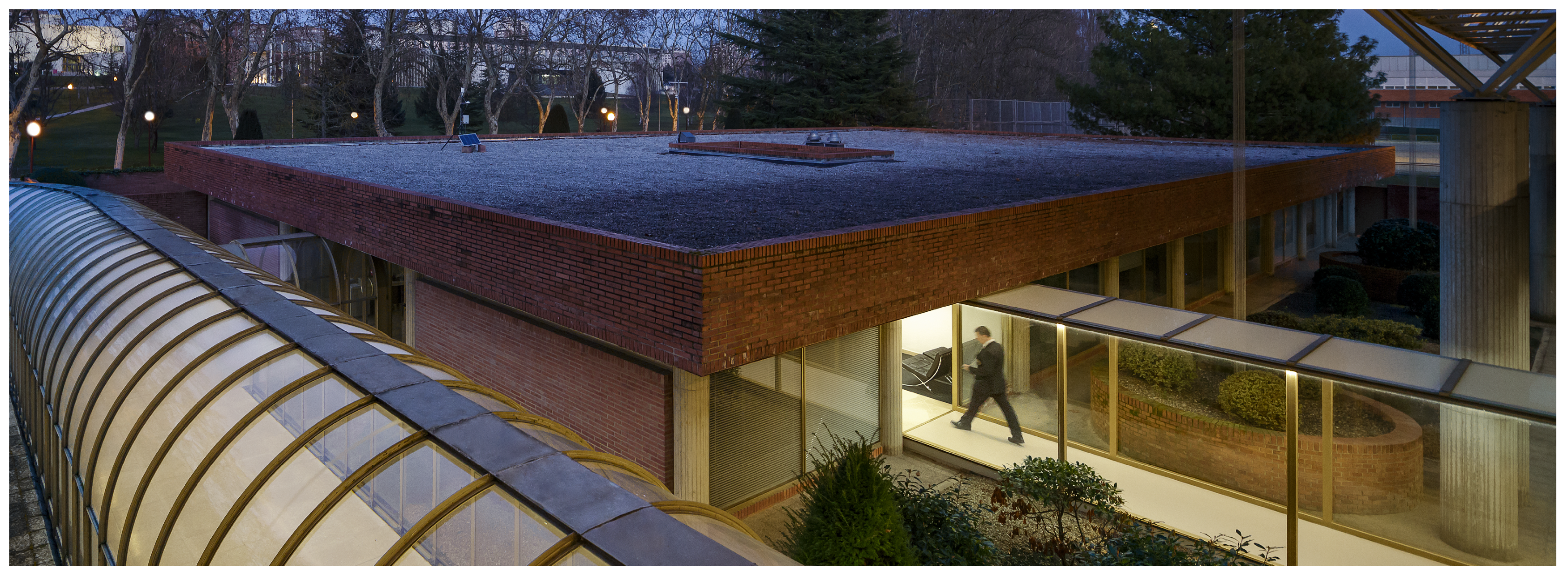
The building selected for generating both case studies explored in this paper was the Architecture School administrative building of the University of Navarra (Figure 1).
The Architecture School was designed by the architects Rafael Echaide, Carlos Sobrini, and Eugenio Aguinaga and was built between 1974 and 1978. It won the “National Award for Architecture in Brick” in 1980. The building is organized along an interior garden with four zones at different levels that accommodate the needs of the school.
Through a transparent gallery, connected to the main building, people can access the office area, which is the building object of this paper. It is mainly used as an administration building and by postgraduate students of the different master’s programs of the School of Architecture, and it mainly keeps business hours.
It is a freestanding single-story building of almost 760 square meters. It is a porticoed structure of concrete, and the interior and exterior walls were made of red clinker brick fabric, while the building frames were made in situ of aluminum with an air chamber and a light gold color.
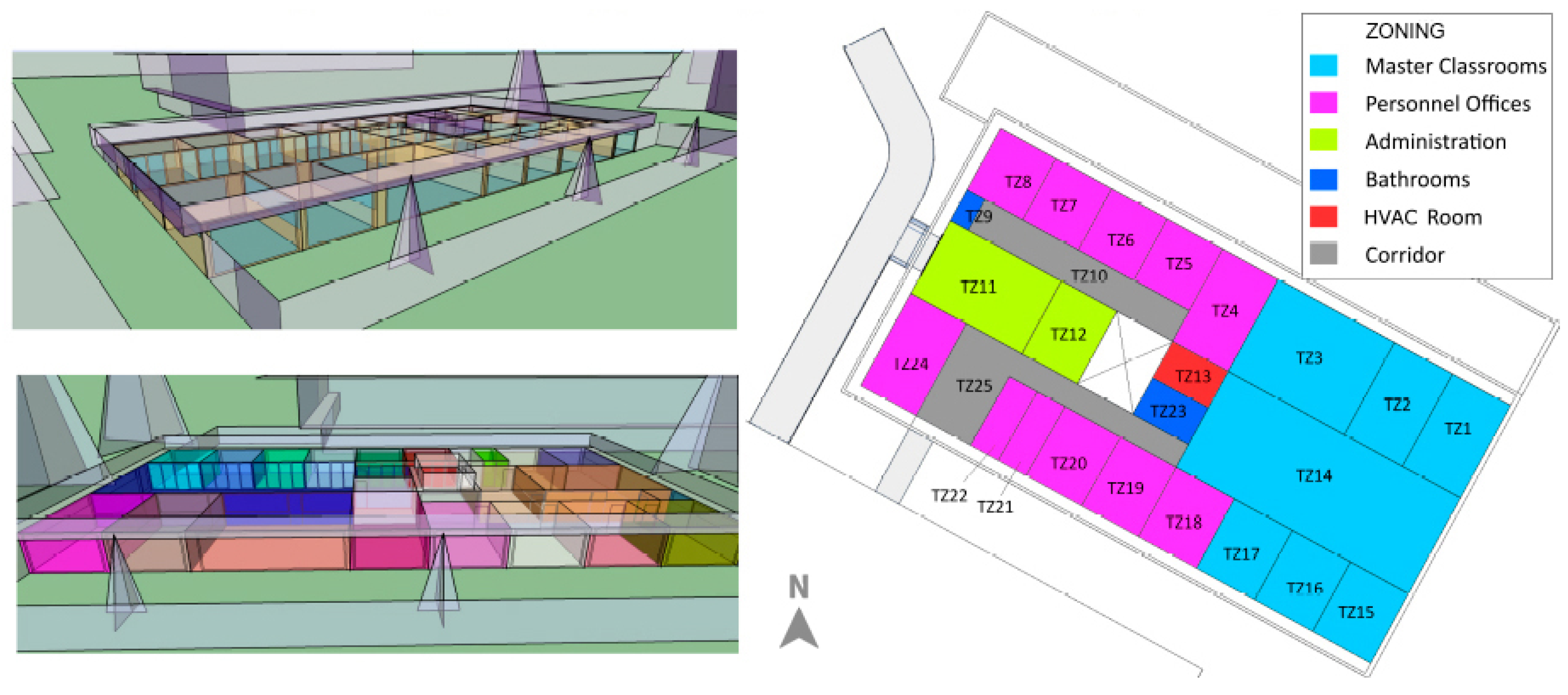
The space allocation consists of a succession of offices for personnel that face southeast and northwest, an administration zone facing northwest, an open working space and master classrooms facing southeast, and a corridor in the middle connecting the spaces.
The building energy model has been divided into 25 thermal zones, one for each room (Figure 2). The HVAC system has been introduced through the option of ideal loads offered by EnergyPlus.
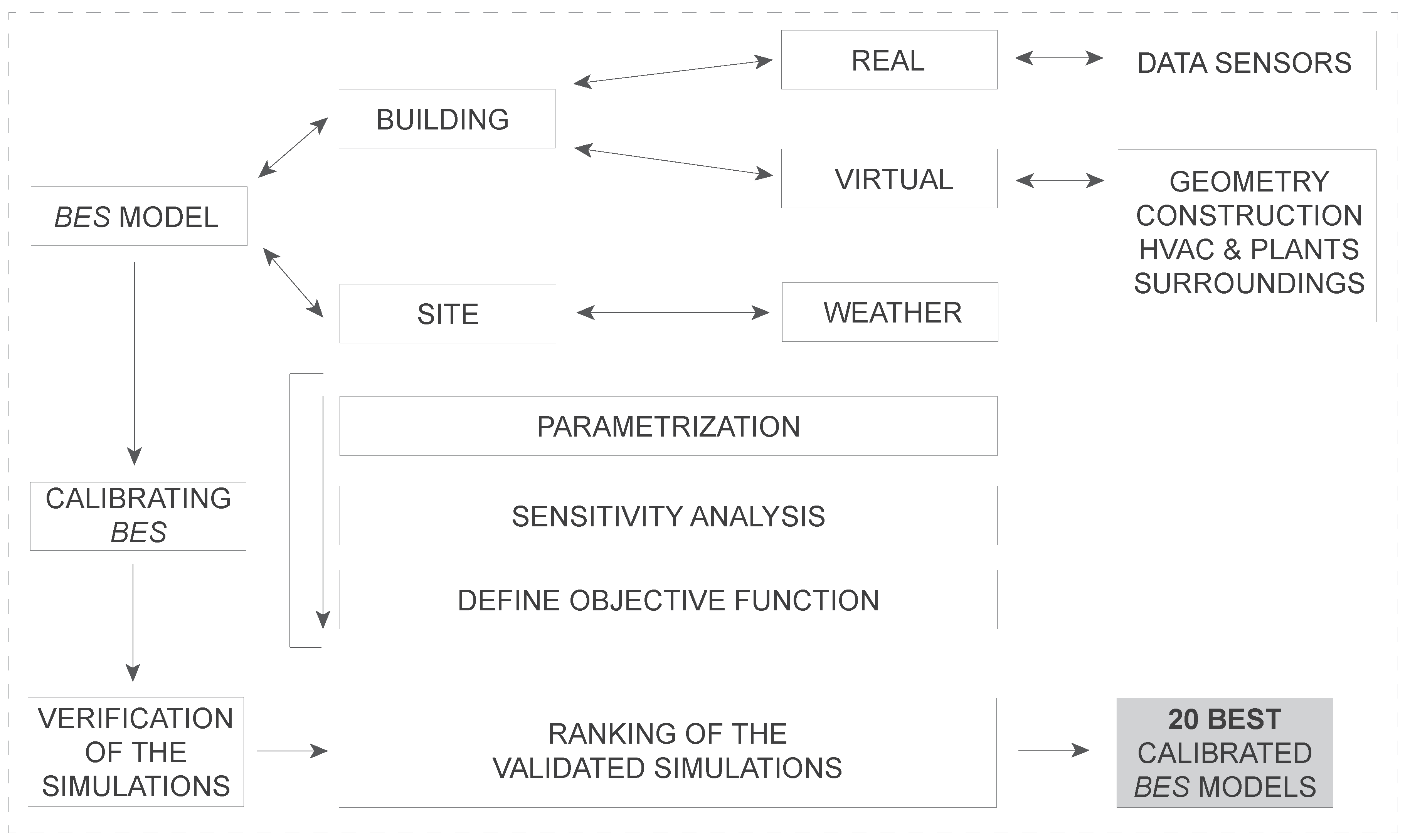
The calibration methodology was carried out by ZEC, described in the previous paragraphs, the process of which is defined in Figure 3.
The last step in the ZEC methodology after calibration is to obtain the 20 best models of the calibration process for each period.

4. Methodology to Evaluate Energy Models: Analysis of Case Studies

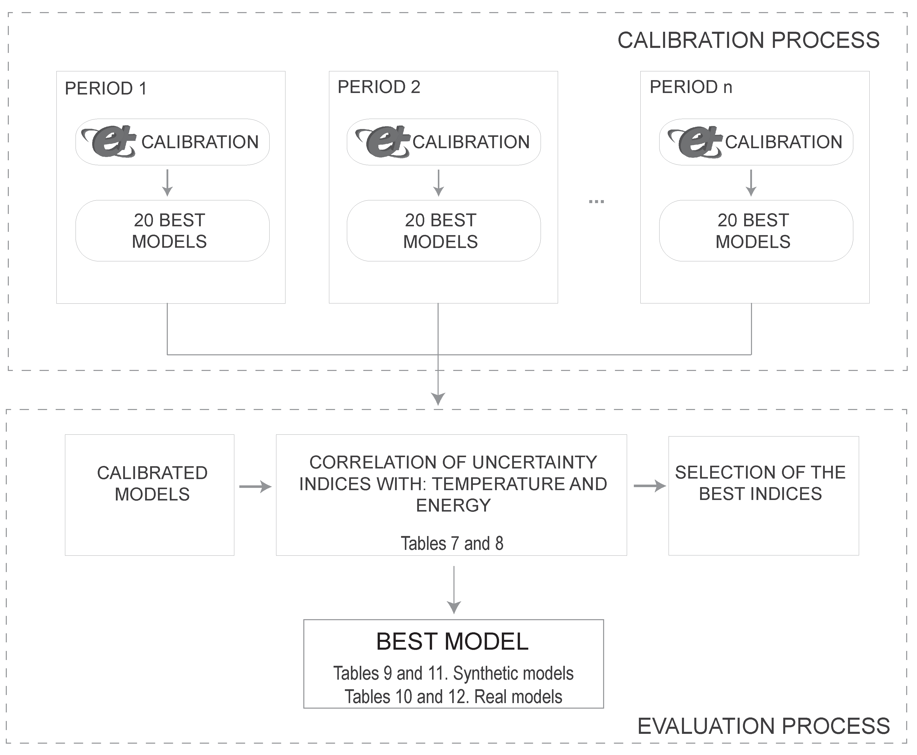
For evaluation of the models, a global checking period is defined to validate the best models of each calibration period. In the ZEC methodology, the evaluation involves performing an uncertainty analysis that compares the simulated temperature during the free oscillation times of the checking period with the measured temperature from the real building. This allows the analysis of all the models on equal terms to generate a ranking of simulations in order to choose the best solution (Figure 4).
To carry out this research, the model has been calibrated, using the ZEC methodology, in 16 different calibrated periods choosing the 20 best models, with the lower energy of each period, generating a total of 320 models. The models have been identified by P k _ M j , where P k is the calibration period (from 1–16) and M j is the model with respect to its position in the energy ranking (from 1–20). These models are evaluated in a common checking period, obtaining the results of their indices of uncertainty and the energy consumed. This study was conducted for both a model with synthetic data and a model with real data.
In the following section, a methodology will be developed to choose the best model among these 320. The methodology proposed a correlation analysis and was performed between the uncertainty indices described in Section 2 and the energy consumption and measured temperature. The energy consumption was calculated from 320 simulations checked over the same period, corresponding to the BEM described in Section 3. The uncertainty indices were calculated using the measured temperatures from a synthetic and a real model in 25 thermal zones.
The correlation was calculated over the mean temperature of these 25 zones, and the real and simulated temperatures were weighted for the relative volume of every zone. Thus, the real ( Y p ) and simulated ( Y ^ p ) mean weighted temperature vectors were defined as:
Y p : = j = 1 25 y i , j V j j V j , Y ^ p : = j = 1 25 y ^ i , j V j j V j
where y i , j and y ^ i , j are the real and simulated temperatures of the thermal zone j at time i and V j is the j-thermal zone volume in cubic meters (35).
For a given model, the best uncertainty indices must have the higher p f a c t o r for small values of λ ; therefore, the correlation between error indices and p f a c t o r ( λ ) could help to identify them. The highest values of these correlations are reached for narrow λ -wide bands, shown in Table 7 for a synthetic model and in Table 8 for a real model.
Another relevant point to determine which indices are appropriate for the best-performing model is the correlation between them and energy consumption. The right column of Table 7 and Table 8 shows the calculated values.
In both cases, there are groups of indices differentiated by the λ -value where they reach the maximum correlation:
  • In the first group, the indices whose maximum correlation is reached at λ = 0.25 for a synthetic model and λ = 1.45 for a real model are measures calculated by the absolute value of the distances.
  • The second group reaches the maximum at λ = 0.3 and λ = 0.45 for a synthetic model and real model, respectively, and they are calculated with squared distances.
  • In the third group, the value of λ varies from λ = 0.05 to λ = 1.35 for a synthetic model and from λ = 0.3 to λ = 1.75 for a real model. They are not related to a specific distance measure.
The indices B E , M B E , and R E are omitted in the results tables since their method of calculation was subjected to cancellation errors and their performance was poor. Another group of indices, A E , R A E , M S E , R M S E , B I C , and the Pearson Correlation Coefficient (r), were omitted because they had redundant information; that is, they were a direct part of the calculation of other measures with equal or better performance, and their correlations were equal to one in the temperature datasets analyzed here. M S E and R M S E had a similar performance to C V ( R M S E ) , and the same happens between the indices pairs: A E and M A E , R A E and M A P E , B I C with respect to A I C , and the Pearson correlation coefficient with respect to the Spearman correlation coefficient.
With the results obtained in the previous Table 7 and Table 8, we can make the selection of the indices for the evaluation of the models. These indices must meet two objectives: good correlation of the indices with temperature and with energy. l o g N S E is one of the indices that fulfills these two premises for a synthetic model and a real model.
Once the indices with which to evaluate the models have been chosen, we proceed to compare them with the old methodology ( Z E C _ i n d e x ) for the proposed cases: synthetic and real.
In Table 9 (synthetic case) and Table 10 (real case), we have the twenty best models ranked by Z E C _ i n d e x (old methodology). In the first one (synthetic case), thirteen out of twenty of these models are among the best of the energy ranking. The best model of Table 9 (P13_M10) was the twenty fifth in the energy ranking.
In the second one (real case), three out of twenty of these models were among the best of the energy ranking. The best model of Table 10 (P10_M2) was the twenty ninth in the energy ranking.
With the new methodology, the results obtained for the synthetic and real case can be evaluated in Table 11 and Table 12. In these tables, the twenty best models are ordered by index l o g N S E . For a synthetic case, Table 11, we can see how seventeen out of twenty of these models were among the best for the energy ranking. The best model of Table 11 (P5_M4) was the tenth in the energy ranking and the number one in the rest of the indices. For the real case, Table 12, ten out of twenty of these models were among the best of the energy ranking. The best model of Table 10 (P9_M8) was the second in the energy ranking and the number one in the rest of the indices.
Depending on the methodology used to choose the best model, the results obtained are different.
For the case of synthetic models, if we rely on the old methodology, the best selected model is P13_M10 and would be ranked twenty fifth in the energy ranking. With the new methodology, the best model was P5_M4 and it had the tenth position in the energy ranking. Analyzing both models, we can see that the model ranked by l o g N S E (new methodology) had a better performance with respect to the temperature curves, as shown by its p f a c t o r , 100% with a λ = 0.2; while the model chosen with Z E C _ i n d e x (old methodology) had a p f a c t o r for a λ = 0.2 of 99.7 %.
The same situation would occur if we analyze the real case. The best model selected with Z E C _ i n d e x (old methodology) was P10_M2 with a position of 29 in the energy ranking, and if we ranked by l o g N S E (new methodology), the best model would P9_M8, being the Number 2 model in the energy ranking. By carefully examining both models, we can conclude that the model classified with the new methodology was better than the one chosen by Z E C _ i n d e x , as shown by its p f a c t o r . The model P9_M8 had a p f a c t o r for a λ = 1 of 90.1 %, while for the model P10_M2, it was 84.7 %.
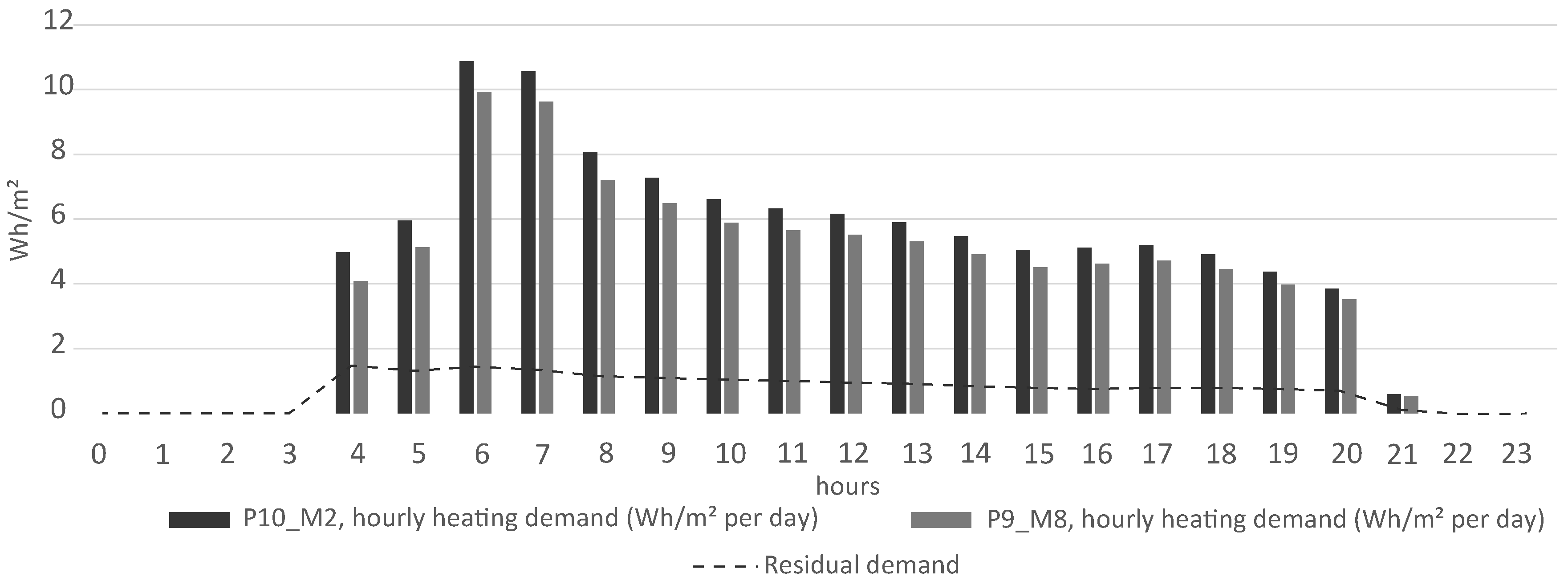
Choosing the best model from a list of calibrated models is crucial in many applications like model predictive control (MPC), where the optimization is based on an hour by hour control of the energy demand of the model in order to reach the goals of the objective function that are related to an increase/decrease of energy consumption during specific time periods. Therefore, having a reliable methodology that gives us this result is paramount. The variation of energy that the two selected models have for the real case, using the old and the new methodology, is significant, as can be seen in Figure 5 and Figure 6, where the accumulated energy at hourly time steps has been represented for heating and cooling demand.

5. Conclusions and Future Research

After obtaining the results of the cases described in the previous sections, it is clear that a single index is not enough in order to select the best model. l o g N S E , r N S E , r d , M A P E , C V ( R M S E ) , c p , and p f a c t o r seem to be the best group of indices to find the best model in both case studies: the synthetic model and the real model. An agreement between all the indices would be desirable in order to choose the best model, as has been demonstrated in this study. In the case of the p f a c t o r , this index not only helps to rank the models, but also can be used as a measure to quantify the quality of the model. This value ( p f a c t o r ) demonstrates the actual gap between the calibration process carried out with synthetic data or with real data.
The results that were presented within Section 4 show that the chosen indices based on M S E ( l o g N S E , r N S E , r d , C V ( R M S E ) , c p ) worked well for time series of temperature data. We estimate that they would still work well in more general scenarios, but some other indices given in this paper could appear to be more appropriate for particular situations. The index l o g N S E had the best correlation between energy and temperature with respect to uncertainty indices in the real case and good performance in the synthetic case. This index was computed after a log-transformation of the data; then it was one minus the ratio between the M S E and the difference between the log of the mean and the mean of the log of the observed temperatures. The r N S E index was again based on a ratio of the M S E and, now, the square of the coefficient of variation of the observed temperatures. Index r d was the ratio between the relative M S E and a kind of M S E comparing the observed and simulated temperatures to the mean of the observed temperatures. The C V ( R M S E ) index was based again on the square of the cover the mean. The c p index was also based on the M S E , now controlled by the consecutive jumps of temperatures. This is especially interesting since it was the only index that took into account the possible correlation between near measures in time. The M A P E index was a relative absolute error index. It can be seen that most of these indices were based on an appropriate ratio of the M S E . Finally, the p f a c t o r was rather intuitive, measuring the observations in a suitable band around the simulated values.
The past results obtained with the Z E C _ I n d e x have been improved with this procedure, as well as the concept of ZEC; calibration by energy was strengthened with this methodology because more models with low energy consumption were among the best models, and there was no uncertainty about the selection of the model in the evaluation process because there was a general agreement between different indices about which one was the best.
A big difference between the synthetic model and real model has been observed, and the new methodology performed better under the real case scenario. This premise has proven to be true, since the methodology presented in this paper is being applied to different buildings and in different calibration periods, showing similar results to those obtained in the previous sections. It is a promising area of research where more calibrated buildings in different environments could be studied. The SABINA project will offer this opportunity.
While in this study, we have used the values of the index to rank the best model offered by the calibration process, in future research, specific values of these indices, in a similar way to that provided by ASHRAE Guideline 14 [16], could be obtained in order to give an idea of the quality of the model. The next generation of BEMs should be classified as complying with the level of quality fed by these indices, depending on the types of applications that are required.

Author Contributions

V.G.G. and L.Á.C. supervised the methodology used in the article, performed the simulations and the analysis, and wrote the manuscript. G.R.R. developed the EnergyPlus model and participated in the data analysis. J.F.L.F. and L.Á.C. developed the methodology that was proposed in the article. All of the authors revised and verified all the manuscript before sending it to the journal.

Funding

The work is funded by the research and innovation program Horizon 2020 of the European Union under Grant No. 731211, project SABINA.

Acknowledgments

We wish to acknowledge the assistance of the University of Navarra (Spain) and, in particular, its maintenance staff for providing us with both the building documentation and data from the sensors placed in it.

Conflicts of Interest

The authors declare no conflict of interest.

Abbreviations

The following abbreviations are used in this manuscript:
ArgArgument
A E Absolute Error
A I C Akaike Information Criterion
B E S Building Energy Simulation
B E Bias Error
B I C Bayesian Information Criterion
b R 2 Multiplied by the coefficient of the regression line (b)
C V ( R M S E ) Coefficient of Variation of R M S E
dIndex of agreement
G o F Goodness-of-fit index
M & V Measurement and Verification process
M A E Mean Absolute Error
M A P E Mean Absolute Percent Error
M B E Mean Bias Error
m d Modified index of agreement
m N S E Modified Nash–Sutcliffe efficiency
M S E Mean Squared Error
N M B E Normalized Mean Bias Error
N S E Nash–Sutcliffe Efficiency
P B I A S Percent Bias
R 2 Coefficient of determination
r d Relative index of agreement
R M S E Root Mean Squared Error
r N S E Relative Nash–Sutcliffe Efficiency
r S D Ratio of Standard Deviations
U I Uncertainty Index
Z E C Zero Energy for Calibration

References

  1. Arcipowska, A.; Anagnostopoulos, F.; Mariottini, F.; Kunkel, S. Energy Performance Certificates across the EU; A Mapping of National Approaches; The buildings Performance Institute Europe (BPIE): Bruxelles, Belgium, 2014. [Google Scholar]
  2. Lewry, A.J.; Ortiz, J.; Nabil, A.; Schofield, N.; Vaid, R.; Hussain, S.; Davidson, P. Bridging the Gap Between Operational and Asset Ratings–The UK Experience and the Green Deal Tool; BRE Group: Watford, UK, 2013. [Google Scholar]
  3. IPMVP Committee. International Performance Measurement and Verification Protocol: Concepts and Options for Determining Energy and Water Savings Volume I; Technical Report; Efficiency Valuation Organization: Washington, DC, USA, 2012. [Google Scholar]
  4. Fernández Bandera, C.; Ramos Ruiz, G. Towards a New Generation of Building Envelope Calibration. Energies 2017, 10, 2102. [Google Scholar] [CrossRef]
  5. Florita, A.; Henze, G. Whole Building Fault Diagnostics—A Bayesian Approach; In Proceedings of the Intelligent Building Operations Workshop, Boulder, CO, USA, 20–22 June 2013.
  6. Haberl, J.; Bou-Saada, T. Procedures for calibrating hourly simulation models to measured building energy and environmental data. J. Sol. Energy Eng. 1998, 120, 193–204. [Google Scholar] [CrossRef]
  7. Dhar, A.; Reddy, T.; Claridge, D. A Fourier series model to predict hourly heating and cooling energy use in commercial buildings with outdoor temperature as the only weather variable. J. Sol. Energy Eng. 1999, 121, 47–53. [Google Scholar] [CrossRef]
  8. Haberl, J.S.; Sreshthaputra, A.; Claridge, D.E.; Kissock, J.K. Inverse model toolkit: Application and testing. ASHRAE Trans. 2003, 109, 435. [Google Scholar]
  9. Kissock, J.K.; Reddy, T.A.; Claridge, D.E. Ambient-temperature regression analysis for estimating retrofit savings in commercial buildings. J. Sol. Energy Eng. 1998, 120, 168–176. [Google Scholar] [CrossRef]
  10. Crawley, D.B.; Lawrie, L.K.; Winkelmann, F.C.; Buhl, W.F.; Huang, Y.J.; Pedersen, C.O.; Strand, R.K.; Liesen, R.J.; Fisher, D.E.; Witte, M.J.; et al. EnergyPlus: Creating a new-generation building energy simulation program. Energy Build. 2001, 33, 319–331. [Google Scholar] [CrossRef]
  11. Sonderegger, R. Diagnostic Tests Determining the Thermal Response of a House; Lawrence Berkeley National Laboratory: Berkeley, CA, USA, 1977.
  12. Vuelvas, J.; Ruiz, F.; Gruosso, G. Limiting gaming opportunities on incentive-based demand response programs. Appl. Energy 2018, 225, 668–681. [Google Scholar] [CrossRef] [Green Version]
  13. Communication from the Commission. A Policy Framework for Climate and Energy in the Period From 2020 to 2030; European Commission: Brussels, Belgium, 2014. [Google Scholar]
  14. Sabina-Project. SABINA. SmArt BI-Directional Multi eNergy gAteway. 2016. Available online: https://sabina-project.eu/ (accessed on 31 May 2019).
  15. Webster, L.; Bradford, J.; Sartor, D.; Shonder, J.; Atkin, E.; Dunnivant, S.; Frank, D.; Franconi, E.; Jump, D.; Schiller, S.; et al. M&V Guidelines: Measurement and Verification for Performance-Based Contracts; Version 4.0; Technical Report; U.S. Department of Energy, Federal Energy Management Program: Washington, DC, USA, 2015.
  16. ASHRAE. ASHRAE Guideline 14–2014, Measurement of Energy, Demand, and Water Savings; ASHRAE: New York, NY, USA, 2014. [Google Scholar]
  17. Giuliani, M.; Henze, G.P.; Florita, A.R. Modelling and calibration of a high-mass historic building for reducing the prebound effect in energy assessment. Energy Build. 2016, 116, 434–448. [Google Scholar] [CrossRef]
  18. Tahmasebi, F.; Zach, R.; Schuß, M.; Mahdavi, A. Simulation model calibration: An optimization-based approach. BauSIM 2012, 1, 386–391. [Google Scholar]
  19. Hong, T.; Lee, S.H. Integrating physics-based models with sensor data: An inverse modeling approach. Build. Environ. 2019, 154, 23–31. [Google Scholar] [CrossRef] [Green Version]
  20. Cipriano, J.; Mor, G.; Chemisana, D.; Pérez, D.; Gamboa, G.; Cipriano, X. Evaluation of a multi-stage guided search approach for the calibration of building energy simulation models. Energy Build. 2015, 87, 370–385. [Google Scholar] [CrossRef]
  21. Bandera, C.F. La Inteligencia Artificial como Inspiración Para la Generación y Diseño de Modelos térmicos de Edificios. Ph.D. Thesis, Universidad de Navarra, Pamplona, Spain, 2016. [Google Scholar]
  22. Bandera, C.F.; Mardones, A.F.M.; Du, H.; Trueba, J.E.; Ruiz, G.R. Exergy As a Measure of Sustainable Retrofitting of Buildings. Energies 2018, 11, 1–19. [Google Scholar]
  23. Manfren, M.; Aste, N.; Moshksar, R. Calibration and uncertainty analysis for computer models—A meta-model based approach for integrated building energy simulation. Appl. Energy 2013, 103, 627–641. [Google Scholar] [CrossRef]
  24. Robertson, J.J.; Polly, B.J.; Collis, J.M. Reduced-order modeling and simulated annealing optimization for efficient residential building utility bill calibration. Appl. Energy 2015, 148, 169–177. [Google Scholar] [CrossRef] [Green Version]
  25. Nguyen, A.T.; Reiter, S.; Rigo, P. A review on simulation-based optimization methods applied to building performance analysis. Appl. Energy 2014, 113, 1043–1058. [Google Scholar] [CrossRef]
  26. Ruiz, G.R.; Bandera, C.F. Analysis of uncertainty indices used for building envelope calibration. Appl. Energy 2017, 185, 82–94. [Google Scholar] [CrossRef]
  27. Farhang, T.; Ardeshir, M. Monitoring-based optimization-assisted calibration of the thermal performance model of an office building. In Proceedings of the International Conference on Architecture and Urban Design, Tirana, Albania, 19–21 April 2012. [Google Scholar]
  28. DoE, U. Energyplus Engineering Reference; The Reference to Energyplus Calculations; EnergyPlus: Washington, DC, USA, 2010.
  29. Wetter, M.; Wright, J. A comparison of deterministic and probabilistic optimization algorithms for nonsmooth simulation-based optimization. Build. Environ. 2004, 39, 989–999. [Google Scholar] [CrossRef] [Green Version]
  30. Chaudhary, G.; New, J.; Sanyal, J.; Im, P.; O’Neill, Z.; Garg, V. Evaluation of Autotune calibration against manual calibration of building energy models. Appl. Energy 2016, 182, 115–134. [Google Scholar] [CrossRef]
  31. Ruiz, G.R.; Bandera, C.F.; Temes, T.G.A.; Gutierrez, A.S.O. Genetic algorithm for building envelope calibration. Appl. Energy 2016, 168, 691–705. [Google Scholar] [CrossRef]
  32. Mustafaraj, G.; Marini, D.; Costa, A.; Keane, M. Model calibration for building energy efficiency simulation. Appl. Energy 2014, 130, 72–85. [Google Scholar] [CrossRef]
  33. Zambrano-Bigiarini, M. hydroGOF: Goodness-of-Fit Functions for Comparison of Simulated And Observed Hydrological Time Series, R Package Version 0.3-8. 2014.
  34. Abbaspour, K.C.; Rouholahnejad, E.; Vaghefi, S.; Srinivasan, R.; Yang, H.; Kløve, B. A continental-scale hydrology and water quality model for Europe: Calibration and uncertainty of a high-resolution large-scale SWAT model. J. Hydrol. 2015, 524, 733–752. [Google Scholar] [CrossRef] [Green Version]
  35. ASHRAE. Fundamentals Handbook, IP ed.; ASHRAE: New York, NY, USA, 2017. [Google Scholar]
  36. EVO. Uncertainty Assessment for IPMVP—Release of a New IPMVP Application Guide; EVO: Washington, DC, USA, 2018. [Google Scholar]
  37. Yoon, J.; Lee, E.J.; Claridge, D. Calibration procedure for energy performance simulation of a commercial building. J. Sol. Energy Eng. 2003, 125, 251–257. [Google Scholar] [CrossRef]
  38. Touzani, S.; Granderson, J.; Fernandes, S. Gradient boosting machine for modeling the energy consumption of commercial buildings. Energy Build. 2018, 158, 1533–1543. [Google Scholar] [CrossRef] [Green Version]
  39. Glasgo, B.; Hendrickson, C.; Azevedo, I.L. Assessing the value of information in residential building simulation: Comparing simulated and actual building loads at the circuit level. Appl. Energy 2017, 203, 348–363. [Google Scholar] [CrossRef]
  40. Chakraborty, D.; Elzarka, H. Performance testing of energy models: Are we using the right statistical metrics? J. Build. Perform. Simul. 2018, 11, 433–448. [Google Scholar] [CrossRef]
  41. Coakley, D.; Aird, G.; Earle, S.; Klebow, B.; Conaghan, C. Development of Calibrated Operational Models of Existing Buildings for Real-Time Decision Support and Performance Optimisation. In Proceedings of the CIBSE Technical Symposium, Edinburgh, UK, 14–15 April 2016. [Google Scholar]
  42. Reddy, T.A.; Claridge, D.E. Uncertainty of measured energy savings from statistical baseline models. HVAC R Res. 2000, 6, 3–20. [Google Scholar] [CrossRef]
  43. Beven, K.J. Rainfall-Runoff Modelling: The Primer; John Wiley & Sons: Hoboken, NJ, USA, 2011. [Google Scholar]
  44. Abbaspour, K. User Manual for SWAT-CUP, SWAT Calibration and Uncertainty Analysis Programs; Swiss Federal Institute of Aquatic Science and Technology, Eawag: Duebendorf, Switzerland, 2007. [Google Scholar]
  45. Kamali, B.; Abbaspour, K.C.; Yang, H. Assessing the uncertainty of multiple input datasets in the prediction of water resource components. Water 2017, 9, 709. [Google Scholar] [CrossRef]
Figure 1. The Architecture School administrative building of the University of Navarra.
Energies 12 02096 g001
Figure 2. Energy model and zoning map of the Office building, School of Architecture (University of Navarra).
Energies 12 02096 g002
Figure 3. ZEC calibration methodology and model evaluation.
Energies 12 02096 g003
Figure 4. Calibration and evaluation process by ZEC for the different calibration periods.
Energies 12 02096 g004
Figure 5. Comparison of heating demand in Wh/m 2 per day in the months of April and May of 2017 of the models evaluated with the old methodology: Z E C _ i n d e x (P10_M2) and with l o g N S E (P9_M8).
Energies 12 02096 g005
Figure 6. Comparison of cooling demand in Wh/m 2 per day in the months of June and July of 2017 of the models evaluated with the old methodology: Z E C _ i n d e x (P10_M2) and with l o g N S E (P9_M8).
Energies 12 02096 g006
Table 1. Bias error measures.
IndexEquation
Bias Error
B E = i = 1 n y i y ^ i
Mean Bias Error
M B E = 1 n i = 1 n y i y ^ i
Relative Error
R E = i = 1 n y i y ^ i y i
Normalized Mean Bias Error
N M B E = 1 y ¯ n p i = 1 n y i y ^ i
P B I A S
P B I A S = i = 1 n ( y i y i ^ ) i = 1 n y i × 100
Table 2. Absolute error measures.
IndexEquation
Absolute Error
A E = i = 1 n y i y ^ i
Mean Absolute Error
M A E = 1 n i = 1 n y i y ^ i
Relative Absolute Error
R A E = i = 1 n y i y ^ i y i
Mean Absolute Percent Error
M A P E = 1 y ¯ i = 1 n y i y ^ i y i × 100 %
E m a x
E m a x = max 1 i n y i y ^ i
Table 3. Square deviations measures.
IndexEquationRangeOptimal value
Mean Squared Error
M S E = 1 n i = 1 n y i y ^ i 2
[ 0 , ) 0
Root Mean Squared Error
R M S E = 1 n i = 1 n y i y ^ i 2 1 2
[ 0 , ) 0
RMSE-observation Standard Deviation ratio
R S R = i = 1 n y i y i ^ 2 i = 1 n y i y ¯ 2 1 2
[ 0 , ) 0
Coefficient of Variation of RMSE
C V ( R M S E ) = 1 y ¯ i = 1 n y i y ^ i 2 n p 1 2
[ 0 , ) 0
R M S E / M A E
R M S E M A E = n i = 1 n y i y ^ i 2 1 2 i = 1 n y i y ^ i
[ 1 , n ] 1
Table 4. Goodness-of-fit measures.
IndexEquationRangeOptimal Value
Pearson Correlation Coefficient
r = i = 1 n y i y ¯ y ^ i y ^ ¯ i = 1 n y i y ¯ 2 i = 1 n y ^ i y ^ ¯ 2
[ 1 , 1 ] | r | = 1
Spearman Correlation Coefficient
ρ = i = 1 n r g ( y i ) r g ( y ) ¯ r g ( y ^ i ) r g ( y ) ¯ i = 1 n r g ( y i ) r g ( y ) ¯ 2 i = 1 n r g ( y ^ i ) r g ( y ) ¯ 2
[ 1 , 1 ] | ρ | = 1
Coefficient of Determination
R 2 = r 2
[ 0 , 1 ] 1
b R 2
b R 2 = b R 2 i f b 1 R 2 / b i f b > 1
[ 0 , ) 1
GoF*
G O F = 1 2 C V ( R M S E ) 2 + N M B E 2 1 / 2
[ 0 , 1 ] 0
Index ZEC
N M B E + C V ( R M S E ) + ( 1 R 2 )
[ 0 , ) 0
Ratio of Standard Deviations
r S D = i = 1 n y i y ¯ 2 i = 1 n y i ^ y ^ ¯ 2 1 2
[ 0 , ) 1
Table 5. Efficiency criteria.
IndexEquationRangeOptimal Value
Nash–Sutcliffe efficiency
N S E = 1 i = 1 n y i y ^ i 2 i = 1 n y i y ¯ 2
( , 1 ] 1
Modified NSE
m N S E = 1 i = 1 n y i y ^ i j i = 1 n y i y ¯ j
( , 1 ] 1
Relative NSE
r N S E = 1 i = 1 n y i y ^ i y i 2 i = 1 n y i y ¯ y ¯ 2
( , 1 ] 1
Logarithmic NSE
log N S E = 1 i = 1 n log y i log y ^ i 2 i = 1 n log y i log y ¯ 2
( , 1 ] 1
Index of Agreement
d = 1 i = 1 n y i y ^ i 2 i = 1 n y i ^ y ¯ + y i y ¯ 2
[ 0 , 1 ] 1
Modified Index of agreement
m d = 1 i = 1 n y i y ^ i j i = 1 n y i ^ y ¯ + y i y ¯ j
[ 0 , 1 ] 1
Relative Index of Agreement
r d = 1 i = 1 n y i y ^ i y i 2 i = 1 n y i ^ y ¯ + y i y ¯ y ¯ 2
( , 1 ] 1
Coefficient of Persistence
c p = 1 i = 2 n y i y ^ i 2 i = 1 n 1 y i + 1 y i 2
( , 1 ] 1
Volumetric Efficiency
V E = 1 i = 1 n y i y ^ i i = 1 n y i
[ 0 , 1 ] 0
Table 6. Comparison model measures. In the equations, d represents the number of parameters of the model.
IndexEquationRangeOptimal Value
Akaike Information Criterion
A I C = n log ( M S E ) + 2 d
R lower value
Bayesian Information Criterion
B I C = n log ( M S E ) + d log ( n )
R lower value
Table 7. (Synthetic case) Group index segmentation by the λ value where the uncertainty indices calculated on weighted mean temperatures and p f a c t o r ( λ ) reach the maximum correlation, in absolute value. The calculated p-values for these correlations are above 0.97 in most cases. The considered λ values are taken within the interval [0.05, 2].
Uncertainty Index (UI)Maximum Correlation between UI and p-Factor ( λ ) Reached at λ Correlation between UI and Consumed Energy
GROUP 1
VE0.99070.250.9055
MAE0.99070.250.9055
mNSE0.99060.250.9055
md0.98950.250.9089
MAPE0.98860.250.9115
GROUP 2
CV(RMSE)0.99230.300.9001
NSE0.99230.300.9001
cp0.99230.300.9001
RSR0.99230.300.9001
d0.99180.300.9015
rNSE0.98970.300.9056
logNSE0.98960.300.9061
ZEC_index0.98980.300.8933
b R 2 0.97790.300.8633
GoF0.99060.300.8818
r.Spearman0.92060.300.9274
rSD0.77200.300.6035
GROUP 3
rd0.98960.400.9081
Emax0.96600.400.9276
R 2 0.91770.400.9611
AIC0.99230.300.9001
R M S E / M A E 0.69990.050.5411
PBIAS%0.58021.350.1628
N M B E 0.58021.350.1628
Table 8. (Real case) Group index segmentation by the λ value where the uncertainty indices calculated on weighted mean temperatures and p f a c t o r ( λ ) reach the maximum correlation, in absolute value. The calculated p-values for these correlations are above 0.95 in most case. The considered λ values were taken within interval [0.05, 2].
Uncertainty Index (UI)Maximum Correlation between UI and p-Factor ( λ ) Reached at λ Correlation between UI and Consumed Energy
GROUP 1
VE0.98111.500.8006
MAE0.98111.500.8007
mNSE0.98111.500.8007
md0.98311.500.8056
MAPE0.98341.450.8220
GROUP 2
CV(RMSE)0.99051.450.8275
NSE0.99051.450.8275
cp0.99051.450.8275
RSR0.99051.450.8275
d0.99071.450.8259
rNSE0.99471.300.8712
logNSE0.99681.200.9137
ZEC_index0.97161.500.7999
b R 2 0.94561.600.7575
GoF0.98971.400.8291
r.Spearman0.96530.450.5900
rSD0.81891.000.8556
GROUP 3
rd0.99411.350.8575
Emax0.98771.750.7260
R 2 0.94840.450.6663
AIC0.99041.450.8275
R M S E / M A E 0.91550.300.4085
PBIAS%0.96350.600.5335
N M B E 0.96350.600.5335
Table 9. (Synthetic case) On the left of the table, ranking ascending by Z E C _ I n d e x and with reference to its energy position. On the right, ranking ascending by energy. The shaded text corresponds to the 20 best energy models.
ModelZEC_IndexEnergy RankingModelEnergy Ranking
P13_M10125P5_M71
P13_M20235P5_M12
P5_M4310P5_M23
P5_M345P5_M94
P13_M15527P5_M35
P5_M868P13_M16
P5_M61212P5_M57
P13_M4814P5_M88
P5_M994P5_M109
P5_M5107P5_M410
P5_M171116P5_M1311
P13_M1126P5_M612
P13_M61322P5_M1413
P5_M10149P13_M414
P5_M2153P5_M1515
P5_M141613P5_M1716
P5_M161720P5_M1117
P13_M91832P5_M1218
P13_M131929P5_M1919
P13_M82030P5_M1620
Table 10. (Real case) On the left of the table, ranking ascending by Z E C _ I n d e x and with reference to its energy position. On the right, ranking ascending by energy. The shaded text corresponds to the 20 best energy models.
ModelZEC_IndexEnergy RankingModelEnergy Ranking
P10_M2129P5_M61
P13_M10219P9_M82
P13_M5330P5_M13
P13_M12439P16_M34
P13_M3545P16_M55
P13_M4646P5_M76
P13_M18731P5_M127
P10_M3884P5_M38
P16_M4910P5_M199
P13_M91047P16_M410
P9_M8112P5_M1011
P13_M11262P9_M1412
P10_M61389P9_M613
P13_M21456P9_M514
P14_M41552P6_M1715
P14_M11663P5_M816
P13_M111781P9_M117
P13_M141875P9_M318
P9_M11923P13_M1019
P9_M22070P6_M1020
Table 11. (Synthetic case) Ranking ascending by l o g N S E . The text in bold corresponds to the models with the lowest energy consumption. The row shaded in gray corresponds to the best model selected by the old methodology.
ModelEnergyMAPErNSElogNSErdp-Factor (0.20)
P5_M4101111100.0%
P5_M352222100.0%
P5_M883333100.0%
P5_M6124444100.0%
P5_M576555100.0%
P5_M945666100.0%
P5_M17167777100.0%
P5_M239888100.0%
P5_M14131099999.8%
P5_M16201210101099.9%
P5_M1098111111100.0%
P13_M15271312121299.9%
P5_M7111131313100.0%
P5_M11171714141499.9%
P13_M10251815151599.7%
P5_M182119161618100.0%
P13_M4141517171699.5%
P13_M161418181799.3%
P5_M19192219191999.8%
P5_M12182320202099.9%
Table 12. (Real case) Ranking ascending by l o g N S E . The text in bold corresponds to the models with lowest energy consumption. The row shaded in gray corresponds to the best model selected by  Z E C _ i n d e x .
ModelEnergyMAPErNSElogNSErdp-Factor (1.00)
P9_M82111190.1%
P9_M1412522387.5%
P16_M552463788.9%
P16_M410334287.0%
P9_M6131255586.9%
P9_M5141146686.9%
P9_M3466127888.5%
P16_M737291181387.8%
P10_M229279484.7%
P9_M417169101084.5%
P9_M3181510111184.5%
P13_M18314812983.3%
P9_M12222113131483.1%
P9_M9241915141582.5%
P13_M10191714151282.1%
P16_M20382518161682.7%
P16_M18485120172584.1%
P9_M11272317181782.8%
P9_M13322016192382.5%
P16_M17684028203082.8%

