Article

The Effects of Regional Fluid Flow on Deep Temperatures (Hesse, Germany)

1
Helmholtz Centre Potsdam GFZ German Research Centre for Geosciences, Telegrafenberg, 14473 Potsdam, Germany
2
Faculty of Georesources and Material Engineering, RWTH Aachen, 52056 Aachen, Germany
3
Institute of Applied Geosciences, TU Darmstadt, 64287 Darmstadt, Germany
4
Darmstadt Graduate School of Energy Science and Engineering, 64287 Darmstadt, Germany
5
Hessian Agency for Nature Conservation, Environment and Geology (HLNUG), 65203 Wiesbaden, Germany
*
Author to whom correspondence should be addressed.
Energies 2019, 12(11), 2081; https://doi.org/10.3390/en12112081
Submission received: 6 May 2019 / Revised: 26 May 2019 / Accepted: 27 May 2019 / Published: 31 May 2019

Abstract

:
A successful utilization of deep geothermal resources requires accurate predictions about the distribution of reservoir temperature as well as of the hydraulic processes exerting a direct influence on the productivity of geothermal reservoirs. The aim of this study was to investigate and quantify the influence that regional thermo-hydraulic processes have on the geothermal configuration of potential reservoirs in the German Federal State of Hesse. Specifically, we have addressed the question of how the regional thermal and hydraulic configuration influence the local hydro-thermal reservoir conditions. Therefore, a 3D structural model of Hesse was used as a basis for purely hydraulic, purely thermal and coupled 3D thermo-hydraulic simulations of the deep fluid flow and heat transport. As a result of our numerical simulations, Hesse can be differentiated into sub-areas differing in terms of the dominating heat transport process. In a final attempt to quantify the robustness and reliability of the modelling results, the modelling outcomes were analyzed by comparing them to available subsurface temperature, hydraulic and hydrochemical data.

1. Introduction

The Federal State of Hesse is located in central Germany being geologically situated at the border between the North German Basin (north Hesse) and the European Cenozoic Rift System (south Hesse). As part of this active rift system, the Upper Rhine Graben is an area of geothermal exploration. The investigation of regional fluid flow and heat transport has been ongoing since decades [1,2,3,4,5,6,7,8]. In Hesse, deep geothermal exploration was unsuccessful so far, despite favorable predictions beforehand [9,10]. This demonstrates that predictions of the deep geothermal potential are associated with large uncertainties. Overcoming such uncertainties requires an understanding of the relevant physical processes driving deep fluid flow and heat transport, as well as the geothermal- and pressure-(overburden-) history, the development of the stress field and the reconstruction of geochemical rock-fluid interactions in the history. In particular the effects of cold recharge and convective upflow of heated fluids on a regional scale [11] need to be better quantified in order to predict geothermal potentials.
To provide an answer to the latter question was the topic of this study. In particular, we have addressed the following question: Which contribution has different heat transport mechanisms in defining the deep thermal field of Hesse? Therefore, we assessed how structural and geological heterogeneities influence deep heat transport and what dynamic needs to be considered if predictions of temperature distributions and flow regimes have to be made. Fault-related convection in sedimentary basins has been well evaluated (e.g., References [11,12,13,14,15,16]). Some of these studies suggest that the lateral influence on the regional thermal field of hydraulically conductive faults is limited (e.g., Reference [15]). We wanted to test the effects of fluid flow without implementing permeable faults.
The heterogeneous geology of Hesse makes the area suitable to study conductive, advective and free convective heat and fluid flow processes, as they are thought to simultaneously occur in the study area. As described in Person et al. [17], hydrological, thermal, chemical and mechanical mass transfer processes are closely coupled in groundwater flow systems in sedimentary basins.
We present results from a data-based high-resolution model of Hesse, which built on former modelling studies [8,18,19,20,21,22]. Herrmann [18] simulated only the fluid flow focusing on the reconstruction of the shallow groundwater surface from hydrogeological data. Freymark et al. [19] introduced a purely thermal model of Hesse to a depth of the lithosphere–asthenosphere boundary (LAB). Later, Freymark et al. [8], published a model which was developed further to include the whole Upper Rhine Graben. For this lithosphere scale model, conductive heat transport and gravity modelling were carried out. In Arndt [20], Bär [21] and Sass and Hoppe [22], a thermal conductive model of Hesse down to a depth of six kilometers was built and in Rühaak et al. [23] this model was combined with geostatistical simulations to include all thermal observation in Hesse. In the present study, the focus was on the physical processes of coupled fluid flow and heat transport. These processes were first quantified separately and then coupled into one simulation to better quantify the transient character of the thermal field evolution. In contrast to the above mentioned earlier studies, the model had a higher numerical resolution. Thus, the fluid flow processes and related effects on the thermal field could be investigated with more spatial detail in three dimensions and on a regional scale.
The Hessian geology is characterized by a diversity of geological domains. Pre-Permian metamorphic crust crops out in the north-west (Rhenohercynian) and crystalline crust in the south-east of Hesse (Odenwald), whereas sediments reach up to 1.4 km thickness in the Hessian Depression (north), and more than 3.8 km in the Upper Rhine Graben (south). The Hessian Depression is part of the North German Basin. Its fill consists mainly of clastic fluvial-lacustrine (Buntsandstein) sediments with thickness increasing northward [24]. In the Oligocene, the Hessian Depression and the Upper Rhine Graben (Figure 1) are believed to have been connected [25,26,27]. In contrast, the volcanic complex of the Vogelsberg structurally and hydraulically separated the southern area of Hesse (Upper Rhine Graben) from the northern Hessian Depression (late Oligocene to early Miocene times) [28,29,30]. The sedimentary series in the northern Upper Rhine Graben can be differentiated into deposits of the Permian Saar-Nahe Basin and the Mesozoic-Cenozoic deposits of the Upper Rhine Graben [31].

2. Input Data

2.1. Structural Model

The structural 3D model of Hesse (Figure 2a, [32]) relied on a large database and was constructed with the modelling software GOCAD [33].
The related database encompassed a digital elevation model, several geological maps, 4150 boreholes, 318 geological profiles and isoline maps of geological layers as well as seismic data ([20] and references therein). This 3D model covered the area of the Federal State of Hesse in South-West Germany from the surface down to 6 km below msl (mean sea level). It differentiated five sedimentary layers and the Variscan crust (Figure 2b). More than 100 faults [34,35,36,37] featuring displacements larger than 50–100 m [21] were represented.
Cenozoic sediments build the uppermost layer and the thickest aquifer. It includes a sequence of aquifers and aquitards in one layer. In the Upper Rhine Graben, the Cenozoic sediments reach up to 3.8 km thickness (thickness maps of the geological units are provided in Supplementary Material Figure S1). Middle to Upper Triassic (Muschelkalk/Keuper) carbonate and sulfate sediments were deposited across the whole area but were eroded in Hesse except for some local occurrences in the grabens. Thereby the Muschelkalk horizontally separates Cenozoic clastic sediments from deeper Buntsandstein sediments locally. The Buntsandstein consists of a sequence of highly permeable sandstones and sandstone-pelite intercalations and shows a thickness of up to 1.4 km in the basin of the Hessian Depression in the North of Hesse. Zechstein carbonates have up to 1.3 km thickness in the North-East and its extension resembles the Buntsandstein in North-East Hesse. The deepest aquifer is the Rotliegend. It consists of clastic sandstones and conglomerates as well as pelite-fine sandstone intercalations with local occurrences of thick volcanic successions of rhyolitic or andesitic composition. Its thickness distribution follows the strike of the innervariscan molasses basin and presents an elongated shape from South-West to North-East with largest thicknesses of about 3 km in the South-West at the eastern border of the Saar-Nahe Basin.
The metamorphic basement below the sedimentary cover is divided into distinct geological blocks, representing different Variscan domains [38] separated by vertical boundaries traced at the surface [39] (Figure 2b). Of these, the North-Western block represents the metasediments and metavolcanics of the Rhenohercynian with the outcropping Rhenish Massif. The central block represents the Northern Phyllite Zone, consisting of low grade metamorphic pelagic to hemipelagic and volcanoclastic rocks [21,40]. The South-Eastern block is the Mid-German Crystalline High with the outcropping Odenwald and consists of mainly felsic granitoids and subsidiary high-grade metamorphic rocks and mafic intrusives of the Odenwald [41]. The Variscan crust is the lowermost layer in the model and reaches up to 6.8 km in thickness in areas, where it crops out.
In summary, three points were characteristic for the structural model of Hesse: (1) The Variscan crust was the only unit present in the entire model domain and crops out in more than one quarter of the area (brown in Figure 2a), (2) stratigraphic gaps occur where sediments had been eroded or not deposited. Such gaps led to (3) “hydrogeological unconformities”, where hydraulically less conductive layers (Middle to Upper Triassic and Zechstein) only partially bound hydraulically the confining conductive layers (Rotliegend, Buntsandstein and Cenozoic). In the south-western model area, the Upper Rhine Graben, only sedimentary aquifers (Rotliegend and Cenozoic) were present, whereas in the Hessian Depression the Zechstein aquitard covered the Variscan crust completely and separated the Buntsandstein aquifer unit from the basement.

2.2. Temperature Database and Previous Thermal Simulations

The temperature database for this work consisted of measured temperatures at the surface and in boreholes at different depths. We augmented the information derived from these data by relying additionally on the results from previous simulations of the thermal field of Hesse. The temperature database of measurements is presented in Appendix A Figure A1.
So far, four 3D thermal models exist, which will be shortly introduced in the following (see also Table 1).
All previous physical models [8,19,20,21,23,32] were built on the base of the same structural model of Hesse of Arndt [20], introduced in Section 2.1. All models predict highest temperatures in South-West Hesse in the Upper Rhine Graben and lowest temperatures in the North [8,19] or North-East [23]. The mathematical model of Agemar et al. [42,43,44] relied on kriging to match available measurement data in Germany. The most recent thermal model of Freymark et al. [8] covered the largest area and included the whole Upper Rhine Graben from the Alps in the South to Hesse in the North. It consisted of 13 geological layers and extended down to the lithosphere–asthenosphere boundary. This conductive thermal model reproduced temperature measurements in Hesse outside of the Upper Rhine Graben with a mismatch of less than plus minus 5 °C. Given the relatively good fit to available measurements, we have opted to make use of the temperature distribution at 6 km as extracted from this model to set the lower boundary condition in our investigation (more detail in Section 3).

2.3. Hydraulic Observations and Previous Hydraulic Simulations

Different datasets were available to set hydraulic boundary conditions as well as to validate the hydraulic model of Hesse. The hydraulic database consists of springs (Figure A2a), the groundwater surface (Figure A2b), recharge data (Figure A3) and hydrochemical investigations, which are described in detail in Appendix B. These datasets were later used for validating the hydraulic model results.
In the central area of the Upper Rhine Graben, a 3D structural model was built by Freymark et al. [7] down to 8 km depth and having a lateral extension of approximately 150 km N-S and 90 km W-E. Freymark et al. [7] and Friedland [45] performed hydraulic and thermo-hydraulic numerical studies based on this model. The main findings of the study by Freymark et al. [7] can be summarized as follows: (i) a general northward flow in the subsurface of the Upper Rhine Graben, (ii) the hydraulic head and permeability distribution is more important than the order of magnitude of permeability of the main border faults, (iii) advective pressure driven upflow in the central part of the Upper Rhine Graben and (iv) recharge at both border faults. The study of Friedland [45] focused on the hydraulic boundary conditions imposed along the model boundaries. The northern and southern vertical boundaries cutting the sediment of the Upper Rhine Graben were assumed as open in one and closed in another scenario for fluid flow. With her work, she could show that the lateral influence of open or closed vertical boundaries in an area, where the general fluid flow crosses these boundaries is only important close to the same borders, but it exerts only a secondary influence to the general flow pattern.

3. Methods

The governing equations of heat and fluid transport were solved within the commercial software FEFLOW® ([46] Version 7.1, DHI WASY GmbH, Berlin, Germany) which relies on the finite element method to numerically solve for transport problems in porous media. The precise formulation is given in Supplementary Material S2.

3.1. Workflow

The workflow to test different fluid and heat transport processes and to identify dominating mechanisms for different areas included several steps (Figure 3). First the thermal (T) and hydraulic (H) field were calculated by means of uncoupled steady-state simulations. Subsequently, both processes were coupled in thermo-hydraulic (TH) steady-state simulations. Therefore the hydraulic head and the temperature field obtained from the uncoupled simulations were used as initial conditions for the coupled steady-state model. In the last step, the time dependency was assessed. Thus, the coupled thermo-hydraulic steady-state simulation result was used as an initial condition for the distribution of the hydraulic head and the temperature. Here density and viscosity were first assumed to be constant. This scenario is carried out to make sure, that the steady-state coupled simulations were in equilibrium. Finally, in the simulation of the highest complexity, density and viscosity variations were considered.

3.2. Numerical Simulation

The numerical mesh generated in FEFLOW® [46] was adopted from Rühaak et al. [23]. They converted the structural model [32] into a highly resolved numerical mesh with an average horizontal resolution of 1 km. Resolution increased locally to less than 100 m. To minimize numerical instabilities in the coupled transient simulation of thermo-hydraulic coupled processes in thick layers, the mesh was additionally refined along the vertical component to reach a lower Finite Element aspect ratio. The coarsest vertical resolution was 1.1 km and the finest resolution was 10 m. According to this, six geological layers were represented by 21 numerical layers (Table 2). As shown by Kaiser et al. [47] the process of mixed convection was most sensitive to the imposed mesh resolution. Therefore, we iteratively refined the mesh in the Upper Rhine Graben until a stable temperature field was obtained independent of the mesh resolution imposed. The average elemental diameter was ~200 m but decreased locally to 8 m in the region of the Upper Rhine Graben. In total, the model consisted of 1,767,129 triangular prisms.

3.3. Properties

To solve the final set of equations, physical, lithology-dependent properties were assigned to all geological units (Table 2). Properties were considered constant for each lithostratigraphic unit, except for the Variscan crust, which was separated into the different Variscan domains. More details on the lithology of the resolved units can be found in Appendix C.

3.4. Thermal Boundary Conditions (BC)

The lateral boundaries were all closed. At the top and at the bottom of the model fixed temperatures were applied as thermal boundary conditions (Dirichlet type BC). At the surface, the annual mean air temperature (Figure A1a, [50]) was used. At the base of the model, we used the thermal configuration after Freymark et al. ([8], Figure 4) at a 6 km depth, thermal effects, resulting from the deep crustal and lithospheric configuration were considered.

3.5. Hydraulic Boundary Conditions

All vertical boundaries and the base of the model were closed to fluid flow. The groundwater surface after Herrmann ([18], Figure A2b) was set as the hydraulic head boundary condition at the top of the model. It varied between 65 and 840 m above msl. That implied that the groundwater surface was at ~100 m below the surface in areas of high elevation (Rhoen, Vogelsberg). In contrast, where the topography was low (Upper Rhine Graben) the groundwater surface was nearly equal to the topography. As the focus of the modelling results lies on deep fluid flow processes, we considered only Darcy’s law for confined aquifers and neglect Richard´s law for unsaturated zones in the uppermost layer.

4. Results

The results of the regional thermo-hydraulic model of Hesse give the first 3D insights on the configuration of the deep fluid flow in Hesse on the whole regional scale. To investigate the thermal field of Hesse with respect to influencing processes of fluid flow, we show results in this section first uncoupled (H and T) and afterwards coupled TH (steady-state and transient taking viscosity and density variations into account), as shown in the workflow in Section 3.1.

4.1. Steady-State Simulations

4.1.1. Hydraulic Steady-State Simulations

As only pressure driven fluid movement was considered in the simulations the resulting regional fluid flow field in Hesse was dominated by flow from higher elevations to lower elevations following the imposed hydraulic gradients at the top surface. Fluid flows with low Darcy velocities (less than 0.1 mm per year) in the Variscan crust, whereas flow velocities were more than two orders of magnitude higher in sediments. The lowest hydraulic heads characterized the Upper Rhine Graben and the Hessian Depression. In both regions, the sediments were thickest. Accordingly, the lowest hydraulic gradients of less than 0.03% in the model area were localized below the Upper Rhine Graben (Figure 5d). The resulting Darcy velocities at intermediate depths were lower in the sediments of the Upper Rhine Graben than in the other sedimentary domains (below 1 mm/a, Figure 5a).
Local flow systems with less spatial extent developed in the Hessian Depression. The topography and the groundwater surface was hilly and thus local hydraulic gradients were alternating between high and low elevations on a small amplitude. This can be seen in Figure 5d, where the hydraulic head isolines are dense and trough-shaped in the Hessian Depression. These hydraulic head variations entailed developing local recharge and discharge areas with a lateral extent of less than 10 km.
Fluids penetrated from the crust into the Rotliegend and Cenozoic sediments following steep hydraulic gradients were the Taunus Border Fault and the Eastern Border fault of the Upper Rhine Graben caused displacements in the structural model (Figure 5b,c).

4.1.2. Thermal Steady-State Conductive Simulations

Considering only steady-state heat transport implies that radiogenic heat production and heat conductivity were the key parameters to produce and distribute heat in the model area. This led to a thermal configuration dividing Hesse into two domains following the borders of Variscan domains (Figure 6). In the north-west, the Rhenohercynian was dominated by low temperatures around 37° at a 1 km depth below msl (Figure 6a) with an average geothermal gradient of 30 °C/km (Figure 6c).
The south-east of Hesse (Mid-German Crystalline Crust and Northern Phyllite Zone) was characterized by higher temperatures around 50 °C at a 1 km depth with locally higher temperatures under the Vogelsberg (66 °C) and Rhoen mountains (60 °C), where the topography was highest. Accordingly, the calculated geothermal gradients increased from north to south by a factor of two. The 100 °C isotherm was at 3.5 km depth in the north under the Hessian Depression and at 2 km depth in the south in the Upper Rhine Graben (Figure 7a). This is consistent with the averaged geothermal gradient of 60 °C/km reported by Agemar et al. [43] for the Upper Rhine Graben.

4.2. Thermo-Hydraulic Steady-State Simulations

In this study, the coupled heat and fluid transport in Hesse were simulated to assess the effects of heat transport on the regional hydraulic flow field as well as the influence of fluid flow on the thermal field in Hesse. When compared to the previously described conductive case, the simulated thermal field differed in the areas characterized by a vigorous fluid flow component. The results depict higher temperatures in the Upper Rhine Graben (60 °C at a 1 km depth) and moderate temperatures where the crust crops out or was covered by thin overlying sediments. Low temperatures were simulated in the Hessian Depression (lowest: 12 °C at a 1 km depth). This regional trend was in agreement with the results of the hydraulic steady-state simulation indicating a pressure driven advective fluid flow component in the Hessian Depression. Indeed, Darcy velocities were highest in this area (Figure 5a). This advective heat transport led to infiltration of cold water and thereby to an overall cooling with respect to the purely conductive case (Figure 6). Therefore, the lowest temperatures were calculated in the North, for the Hessian Depression. These temperatures were up to 15 °C colder at a 1 km depth than in the conductive simulations.
The temperature distribution at 1 km depth (Figure 8a) showed the highest temperatures in the south, i.e., in the Upper Rhine Graben. There, the magnitudes of simulated temperatures were in the same range (around 60 °C) as obtained from the uncoupled thermal simulation (Figure 6a). Cold temperatures were predicted at the Eastern Graben Border Fault and at the Southern Taunus Border Fault, Figure 8a. The results of Figure 8a indicate lower temperatures along both structural steps. Moreover, Figure 8c indicates downflow zones at exactly these two locations. Accordingly, colder temperatures at these two faults were the result of groundwater inflow from high elevations following the hydraulic gradients in the sediments of Rotliegend and Cenozoic.
Moderate temperatures were predicted in the northwest, where the Variscan crust was only locally covered with sediments. Moreover in the East, where the crystalline crust was the dominating geological layer of the model and sediments were thinner than in the Hessian Depression (North), Vogelsberg (central Hesse) and Upper Rhine Graben (South) regions. In more detail, Cenozoic, Muschelkalk and Rotliegend sediments were missing in the East (or very thin, Figure S1a,b,d in Supplementary Material S1) and Buntsandstein and Zechstein with up to about 700 m cover the Variscan crust. In these areas (northwest and east), the Darcy velocities were the lowest (Figure 8b). While Darcy velocities between 1 and 10 mm per year were predicted in the Upper Rhine Graben, Darcy velocities in the Hessian Depression were generally higher (up to 100 mm per year). This is consistent with the fact that the assigned hydraulic conductivity in the Cenozoic sediments in the Upper Rhine Graben is lower than that of the Buntsandstein aquifer of the Hessian Depression. As described in Section 4.1.1, local flow systems evolved in the Hessian Depression because of the hilly topography in contrast to very low hydraulic gradients in the Upper Rhine Graben resulting in low fluid velocities. Accordingly, the hydraulic head isolines shown in Figure 8d are closer in the North and illustrate the development of local flow systems with recharge and discharge areas on a smaller spatial scale. In contrast, isolines were very wide and the Darcy velocities were lower in the southern part of the profile (Figure 7d; between 0 and 60 km profile length). This pattern was not influenced by the conductive heat transport and was observed as well in the purely hydraulic simulation beforehand (Figure 5d). On the other hand, the thermal configuration in the Hessian Depression changed from the conductive case to the thermo-hydraulic simulation. The temperatures in the conductive case were predicted between 37 and 45 °C (Figure 6a) and in the coupled case around 12–25 °C (Figure 8a) at 1 km depth. The conductive field in the Hessian Depression was influenced by advection in contrast to the thermal field in the Upper Rhine Graben. Here the thermal configuration did not fundamentally change from thermal to thermo-hydraulic simulations (see also Figure 7). The predicted temperatures at 1 km depth were in both cases around 60 °C (Figure 6a and Figure 8a). Only locally at the Eastern Main Border Fault did temperatures cool down to less than 30 °C at 1 km depth (Figure 8a).
One more difference between both regions (Upper Rhine Graben and Hessian Depression) was the varying basal heat input implemented in the simulations by the lower boundary condition [8]. Higher temperatures were located below the Upper Rhine Graben and lower temperatures were observed below the Hessian Depression.

4.3. Transient Thermo-Hydraulic Simulations

4.3.1. Transient Simulations with Constant Viscosity and Density

In an attempt to validate the steady-state nature of the resulting thermal and hydraulic field as described in the previous paragraph, we performed additional transient simulations. In these runs, we did not consider any variations in the fluid density and viscosity, therefore no buoyancy effects were considered in the flow. In addition, we used the thermal and hydraulic head configuration as derived from the steady-state thermo-hydraulic simulations as initial conditions. Maps of Darcy velocities at a 1 km depth showed constant values over time (Figure 9a–c). Consistent with these results, also the thermal field in these areas did not change over the simulated time frame (Figure 10a–c).

4.3.2. Transient Simulations including Density and Viscosity Variations

In a final stage, we considered the additional effects of fluid density and viscosity variations (mixed convective regime) on the regional thermal and hydraulic field. Following this process, higher fluid temperatures translated into the fluid being lighter and therefore they might lead (depending on the permeability configuration) to fluid rising following the resulting density gradients. This might also lead to mixing of fluids of different origins within the different sedimentary layers thus influencing the temperature distribution. In order for this process to be effective, some hydrogeological conditions were encountered. These comprised a relatively high aquifer thickness and hydraulic conductivity and relatively low hydraulic head gradients [51,52]. Within the study area, these hydrogeological conditions were fulfilled in our simplified model in the Upper Rhine Graben. There, a homogeneous thick aquifer layer of more than 3 km of Cenozoic sediments with an assumed high hydraulic conductivity (1 × 10⁻⁷ m/s), neglecting internal layering and permeability variations of the different lithostratigraphic were found in an area of the low surface hydraulic gradient. Moreover, a high geothermal gradient was also present in the Upper Rhine Graben leading to favorable conditions for the onset and maintenance through time of convective processes.
In the simulation results, locally increased Darcy velocities in the Cenozoic sediments of the Upper Rhine Graben (Figure 9d–f) can be observed. Flow velocities in thermal uprising zones reached Darcy velocities of 1 m/a. These localized uprising zones (convection cells hereafter) developed over a simulation time of 100,000 years. Moreover, in Figure 10d–f the temperature maps at 1 km depth show differences in the temperature distribution in the area of the Upper Rhine Graben. Mixed convection led to locally higher temperatures in the Upper Rhine Graben when compared to the purely advective regime, with the temperature reaching 90 °C after 100,000 years of simulation time, what means 30 °C higher than in the advective and conductive simulation (Figure 10f,i). Where the deep heated water was locally ascending, the temperatures were higher. There was an opposite effect as well, enclosing the areas of uprising fluids the temperatures cooled down. The hot water cooled down at the top, descends and transports cold water in deeper areas (Figure 10e,f: purple areas in the Upper Rhine Graben). The cooling evolved over time and was most efficient after 100,000 years. In detail, the cold areas in the Upper Rhine Graben had temperatures at a 1 km depth around 30 °C, locally down to 15 °C (Figure 10g–i).
The thermal and flow configuration outside of the Upper Rhine Graben did not change considerably when considering the free convection. Therefore we can conclude that the remaining areas, that is, the areas outside of the Upper Rhine Graben were not affected by the process of mixed convection.
A closer look on the results of simulations with variable density and viscosity in the northernmost part of the Upper Rhine Graben shows that the overall fluid movement is almost the same as obtained for the simulations having constant density and viscosity (Figure 11). Indeed, we observed the same pressure driven fluid movement in the Upper Rhine Graben. Fluids downflow along the Eastern Graben Border Fault and they ascend along the Western Graben Border Fault (Figure 5b and Figure 11a). Additionally to this advective flow component, we were also able to model an upwelling flow located at the center of the graben (Figure 11a).
The upflow zone along the Western Graben Border correlates with an increase in temperatures (illustrated in Figure 10i). At this location, fluids flow from the eastern flank into the central domain of the graben where it finally leads to an overall cooling. At locations where the base of the sedimentary rocks was offset along the structural crustal steps, heated fluids ascended transporting heat upwards.
Figure 11a illustrates a west-east profile, which crosses the northern Upper Rhine Graben perpendicular to the graben axes cutting the Variscan crust at the base, Rotliegend sediments above and Cenozoic sediments as uppermost graben fill layer. It illustrates the graben perpendicular flow directions. The fluids infiltrated at the Eastern Graben Border Fault, following the hydraulic head gradient and thereby transport cold surficial water into the graben at depths. This flow, driven by advection was already present in the steady-state hydraulic (Figure 5c) and thermo-hydraulic simulations. The results of the free convective transient model show a changing of fluid pathways in the central part of the graben, where fluids locally ascend nearby a step in the adjacent crust. In the western half of the graben, a similar hydraulic pattern can be observed. Fluids followed the hydraulic gradient (close to the Western Graben Border) and ascended along the graben border moving along the Western Graben Border.

5. Discussion

5.1. The Deep Thermal Field Underneath Hesse–Physical Processes and their Influence

The aim of this study was to quantitatively assess which heat transport processes affect the deep thermal field of Hesse, and therefore to identify areas where each specific heat transport mechanism, whether conduction, advection and convection, exerts the primary control on the thermal field. By relying on a systematic numerical analysis we were able not only to assess their respective influence on the overall thermal and hydraulic configuration but also the results from their nonlinear coupling. Based on the obtained results, we were able to subdivide the study area in two main subdomains in terms of the relevant hydrodynamics: a conductive dominated domain characterized by the presence of low permeable units; and, a domain where fluid mediated, whether advective or buoyant, heat transport processes exert primary controls where permeable geological units were present (Figure 12).
Heat conduction is the dominating heat transport mechanism in areas where the Variscan crust crops out or where the overlying sediments are relatively thin (shown by the red shaded areas in Figure 12). These regions are mainly found in the Rhenish Massif (northwest of Hesse). A second region where diffusive heat transport is the dominant mechanism can be found in the Odenwald (southeast Hesse) and Spessart (north of Odenwald). Beneath these areas, the Variscan crust is characterized by a relatively low hydraulic conductivity (7.9 × 10⁻¹² m/s) resulting in low fluid velocities (0.01–0.1 mm/a). Accordingly even when accounting for the additional role of fluid flow, it does not lead to any sensible modification to the overall (conductive) thermal regime. Within an overly conductive regime, the temperature distribution at depths is influenced to a first order by the spatial distribution of the main thermal rock properties, that is, rates of radiogenic heat production and thermal conductivity. As already demonstrated in previous studies by Freymark and co-workers [8,19], the conductive heat transport shows a high degree of structural inheritance, in which variations in the thermal patterns reflect the crustal zonation from Variscan times. By integrating this first order level of structuration at crustal levels, the temperature measurements could be reproduced by our modelling results (see also Section 5.2.1). The quality of the relative fit between measurements and numerical results provides robust, being insensitive to the degree of couplings in the different model runs, thus giving indications of the reliability of the modelling results for these domains.
The situation changed when moving towards areas of relatively thick and permeable sedimentary units (Cenozoic, lower Triassic Buntsandstein and middle Permian Rotliegend). The thermal field underneath these areas was found to be highly sensitive to the additional fluid mediated transport component, thus being highly coupled to the local-to-regional hydraulic regime. With respect to the latter, it should be noticed that these domains correspond also to the highest surface hydraulic gradients in the whole study area. Fluid mediated advection beneath areas of high hydraulic potential causes infiltration of surficial cold water, which penetrates in the underlying aquifers at different depth levels depending on the magnitude of imposed gradients. This leads to an overall cooling in the subsurface temperature distribution for the runs where these advective components have been taken into account. The temperatures at 1 km depth below the surface were lower than 35 °C (Figure 13f), locally decreased to 12 °C, in the Hessian Depression (Figure 8a). Below the Vogelsberg and at the Eastern Border Fault of the Rhine Graben a similar trend was observed with the runs considering pressure forced infiltration of cold water leading to colder temperatures at these locations with respect to purely conductive simulations. Comparing simulated temperatures from the thermo-hydraulic advective model with temperature measurements indicates that predicted temperatures generally underestimate measurements (in more detail in Section 5.2.1). However, when comparing the simulated groundwater dynamics to available observational constraints derived from hydraulic and hydrochemical investigations, the model results were able to reproduce the overall dynamics with groundwater recharging the system at the Odenwald, descending along the Eastern Graben Border into the Upper Rhine Graben sediments, and flowing perpendicular to the main graben axis to the Western Border where it finally ascends. Moreover, the simulations predict infiltrating cold surface water along the Taunus Border Fault following head gradients, but for local upflow areas, the latter correlating spatially with thermal springs.
The highest degree of complexity in this study was solved by additionally considering buoyant flow driven by fluid density gradients. Following density gradients, hotter and thus lighter fluids tend to ascend thereby transporting heat towards shallower depth levels. Onset and stability conditions for this heat transport mechanism are to be related to favorable hydrogeological conditions like the critical thickness of permeable and homogeneous layers and low, if not negligible hydraulic head gradients. These conditions are fulfilled only in specific local domains within the study area, specifically in the Upper Rhine Graben along the southern model boundary. Therefore, free convection exerts a rather local influence on the regional thermal configuration, being limited to the southern portion of the model domain (white area in Figure 12). There, free convection perturbs the temperature field (Figure 13g) and leads to a rather complex temperature distribution that substantially differs to the results from previous studies that did not take this additional heat transport mechanism into account [8,19,21,23]. With respect to the previously described modelling scenarios, the results of this simulation are overly similar to the advective modelling results but differ only in the Upper Rhine Graben. The local uprising of deeper fluids by buoyancy underneath these areas closely resembles observations done in previous hydrogeological investigations pointing to the uprising of salty water along the Western Graben Fault [53]. Indeed, along this branch of the fault, an elongated thermal anomaly develops causing deeper seated thermal water to ascend towards shallower levels (Figure 11a).
When looking at the modelling results with a regional perspective, simulated temperatures (trends and magnitudes) agree with the major outcomes from previous studies ([8,19,21,23] in Figure 13a–d). Highest temperatures were predicted below the Vogelsberg and in the Cenozoic sediments of the Upper Rhine Graben, while lowest temperatures are predicted for the area North-West of Hesse. Despite these trends being preserved in the current study, our results point to the presence of domains of finite extent where this general trend is overprinted by the local groundwater dynamics. These are areas where the local hydrogeological configuration favors the onset of additional heat transport mechanisms (mainly free convection and short wavelength forced convection), thus resulting in a rather peculiar thermal configuration. An example of such specific areas is represented by the Vogelsberg, where the results from the different runs predict quite opposite temperatures. While based on a purely conductive model, this area sees relative high temperatures, the additional influence of fluid mediated transport mechanisms drastically changes the modelling outcomes. This disagreement points to the need to carefully revisit the model parameterization, mainly in relations to imposed variations in hydraulic permeability. Therefore, given the current data availability, we could only provide a quite generic conclusive remark when comparing the modelling results with other hydrogeological constraints. The high recharge at the Vogelsberg (data shown in Appendix B, Figure A3) indicates relatively high infiltration rates of surface water into the underground. This points towards a hydrothermal regime control to a high degree by the local hydraulic conditions as also testified by the presence of local thermal manifestations (springs) in the area.
Despite these local differences, we could conclude that our results corroborate the current understanding of the regional configuration of the study area within two main domains, that is, a domain characterized by higher temperatures in south Hesse bounded by a region of lower temperatures in north Hesse also consistent with available temperature data.

5.2. Model Validation

In a final attempt to validate the obtained simulation results, we carried out a comparison of the modelling results with available thermal, hydraulic and hydrochemical data.

5.2.1. Predicted Versus Measured Temperature Data

Simulated temperatures were compared to available temperature measurements in wells (details on the database in Appendix A). In Figure 14, the 3D distribution of differences between simulated and measured temperatures are illustrated (illustrated are only the results from the last model realization considering all main transport processes). Spheres are color-coded according to the relative misfits between simulated and measured temperatures, with each sphere representing one measurement. Areas, where the thermal field is dominated by conduction show the highest level of agreement with available temperature data. In a similar manner, also the temperature distribution in the domain to the east, where fluid mediated heat transported by pressure gradients is also active was captured by the modelling. In the area of the Hessian Depression, the deep temperatures were underestimated by the model. This could be related to an oversimplification in the parameterization of the Buntsandstein aquifers, considered homogeneous. If interbedding lower conductive layers (as upper Buntsandstein-Röt) would be implemented, the cooling effect of infiltrating surface water would be restricted to the shallow aquifer domains thus resulting in higher temperatures with depths. The Upper Rhine Graben is the area of highest mismatch between modelling results and temperature measurements. Once again, such a mismatch is to be associated with oversimplifications in the hydrogeological parameterization adopted. The permeable layer of Cenozoic sediments with a high thickness of more than 3 km was parameterized as a homogeneous isotropic layer. The topography within the Upper Rhine Valley is nearly flat. Even though the hydraulic gradient is high at the Eastern Border Fault of the Graben, it smooths out in the graben itself. This results in low magnitudes of flow velocities as modelled assuming a steady-state thermo-hydraulic simulation (Figure 8b), and in a negligible week influence of the advective transport component in this area. Density and viscosity variations lead to an additional destabilization of the layered conductive thermal field in the Upper Rhine Graben (Figure 10d–i). The results indicate that the mechanism of free convection is able to perturb those areas where the impact of advective fluid flow on heat transport is minor, that is, underneath areas of small magnitudes hydraulic head gradients. 64% of the measured temperatures could be predicted with a misfit of less than 5 °C and 81% with a misfit of less than 10 °C. Not surprisingly, in the Upper Rhine Graben, the misfit between measured and predicted temperatures was the largest. This misfit was mainly limited to depth levels down to 1 km below the surface, where predicted temperatures overestimated measurements by more than 20 °C. This has to be attributed to convection processes which bypass the whole Cenozoic unit, due to simplification of its hydrogeologic characterization. In order to be able to improve the fit between model and observations for these specific areas, would require detailed models with higher resolutions.

5.2.2. Predicted Flow Field and Hydraulic Observations

A quantitative comparison of hydraulic data with the modelling results is more complicated than for the temperature measurements as described above. This stems from the hydraulic dataset being heterogeneous consisting of four different subsets (detailed information on the dataset is given in Appendix B). The first is the groundwater pressure surface (by Herrmann [18]), the second is the spatial location of 1562 springs plus eight hot springs (by the HLNUG, Figure A2), the third are two different datasets of groundwater recharge rates (by Kopp et al. [54] and the Federal Institue for Geosciences and Natural Resources, Figure A3) and the fourth are results and interpretations derived from hydrochemical investigations. The first dataset was used as an upper boundary condition in all models. Therefore it cannot be used for validation purposes. In order to make use of the second dataset for spring and hot spring locations, we make a qualitative comparison between their locations and the modelled groundwater dynamics (upflow and downflow areas, Figure 15).
In Figure 15, the vertical component of the fluid flow is shown averaged over the entire depth of the model domain. The pattern of up- and downflow areas correlate with the topography and the upper hydraulic boundary condition of the groundwater pressure surface (Figure A2). Assuming, that springs can be used to trace local upflow areas or at least areas having lower hydraulic potential favoring local discharge, we compared their locations with the trend provided by the computed streamlines (red colors in Figure 15 indicate an upflow component and blue colors a downward component). The most valuable data for model validation in this context, are those of the hot springs since they indicate locations where thermal water ascend at the surface from the deeper underground. The four hot springs, observed at the Taunus Border Fault (hot springs: 1–4 in Figure 15), correlate spatially with locations, where the model predicts ascending fluids. Two hot springs in the Hessian Depression (Figure 5 and Figure 6) were also observed at locations where the advective simulation predicts upflow areas. The hot springs at the Vogelsberg (7) and in the Taunus in south-west Hesse (8), did not clearly correlate with any modelled upflow zone.
The spring data comprise a signal which integrates both shallow groundwater, which percolates through small fractures and a deeper origin. This said, and given the fact that it is not clear how to separate the two components, we do not make any systematic analysis of these data, if not to provide an additional, though rather a qualitative constraint to the modelling results. In Southeast Hesse, many springs were measured in the crystalline Odenwald but these springs are not reproduced by the model. The crystalline crust of the Odenwald is parameterized with low hydraulic conductivities. This leads to a conductive dominated regime at the Odenwald where fluid flow-mediated heat transport being of secondary influence. Unfortunately, no temperature data (Figure A1) in the Odenwald were available, which could have been used to cross-validate the reliability of the modelling results in this area. Therefore, we could not be conclusive on the nature of the surface hydraulic manifestation if not relying on additional data, whether from temperature boreholes or hydrochemistry analysis which are missing at the moment.
The free convective thermal field in the Upper Rhine Graben cannot at all be validated with this spring dataset, because we had no available spring data (see Figure 15). The spring data correlate very well with the upflow areas in most parts of the Hessian Depression, what could be explained with the correct characterization of the area as an advective dominated system. The springs at the southern flank of the Vogelsberg are predicted with the advective process model very well, which leads to the conclusion that the southern part of the Vogelsberg was well parameterized as a permeable layer. At the northern part of the Vogelsberg, the springs werenot reproduced, which led to the interpretation that there the parameters were different from the southern part and the lithology probable changes. According to Leßmann [55], the groundwater pressure head beneath the Vogelsberg is nearly flat and the groundwater aquifers above are all uncoupled from the deep fluid flow. This would explain the predicted too low temperatures at the Vogelsberg (Figure 13f,g) of about 10 °C at 1 km depth. The advective infiltration, which results in the high heads at the Vogelsberg (according to Herrmann [18], Figure A2), would be much weaker if the head boundary condition would be lower in this area. In the East of Hesse, there is no clear fit or misfit of the upflow zones and the springs. However, as the conductive model predicts the measured temperatures very well there, we assumed a conductive heat transport regime and negligible fluid flow in the deep underground.
The third set of hydraulic data comprise groundwater recharge rates [54,56], which can be systematically correlated with simulated up- and downflow areas under certain assumption made on the surface hydrological system. In the current study, we assume that magnitudes of groundwater recharge rates provide a conservative measurement of the amount of percolating water in the unsaturated zone. Therefore they should map areas of downflowing water in the simulations and vice versa. High recharge rates can be observed in high elevation areas like Rhoen, Vogelsberg and Odenwald, where the models predict the potential for surface fluid to penetrate into the model domain. Moreover, at the Eastern Graben Border Fault, the recharge data indicate high infiltration rates, observational evidence that coincides perfectly with the simulated advective downflow at the Eastern Border Fault into the graben sediments (Figure 8c).
The fourth observational dataset for the validation of the hydraulic field is different hydrochemical investigations that have been done in the study areas [16,53,57]. Results from hydrochemical and isotope analyses of sampled groundwater have been interpreted to provide a conceptual hydrological model in which groundwater recharge takes place in the Odenwald area, following topography gradients into the Upper Rhine Graben valley. These fluids are thought to uprise at the Western Main Border Fault [16,57]. Geomagnetic and geoelectric methods were used as further proof of this conceptual model, specifically to “validate” the potential of the uprising of salty water at the Western Border Fault [53]. These interpretations could be reproduced with the purely advective hydraulic and with the thermo-hydraulic models.

5.3. Limitations of the Current Study and Ongoing Activities

The study presented in this contribution is of a regional nature, the aim of which was to investigate the regional fluid flow patterns within the study area. Modelling the regional flow and thermal field of a complex area comes necessarily with some simplifications. In the following, these simplifications are discussed with respect to the main conclusions drawn in this study.
On the basis of the investigations by Freymark et al. [7] and given the recent in situ stress field in the area, we also assumed that the main border faults of the Upper Rhine Graben would not exert any first order influence to the overall fluid and thermal field in this region. However, the impact of second-order families of geological discontinuities cross-cutting the graben on the local flow systems has not been systematically investigated so far. From the results obtained so far, we can be positive in stating that such fault zones would not drastically change the regional flow patterns as outlined in this study, though they might be important on a more local scale.
The prediction of the exact locations and of the time-dependent evolution of thermal anomalies in the Upper Rhine Graben is at the time of writing still hindered by some limitations intrinsic in the numerical analysis. While we have been able to demonstrate for the first time that under specific hydrogeological conditions, thermal anomalies of convective nature might develop, no conclusions could be derived on their stability over geological time scales. This is mainly related to the lack of proper temperature dataset which could cover the relevant temporal scales of the processes being investigated. In addition, the resolution of the current model also provides additional limitations in systematically investigating the details of such convective processes. This aspect calls for more local, therefore refined investigations which could also add some of the degrees of freedom missing in term of the local geological configuration as represented by minor faults and their impact on the local convective circulation. This said, we could be positive in this work while stating that our regional analysis has been able to pinpoint specific areas where free convective heat transport is expected to occur, thus providing physics-based guidelines for additional future activities.
Using a Federal sSate boundary as model boundary came with some complications because it hinders to include the whole extent of the catchment areas. The western border of the federal state boundary is crossing the crystalline crust (Rhenish Massif) and can be assumed as hydraulically impermeable. Similarly, the eastern border crosses the Rhoen, where the sedimentary layers are thin and can be seen as a closed boundary as well. In the south, the Odenwald is a groundwater divide as well. In areas, where the thick sediments of the Hessian Depression (north Hesse) and of the Upper Rhine Graben (south Hesse) are present, it could be critical to close the borders as based on political borders. This is specifically problematic in south-east Hesse, where the river Main is entering the model domain. A better approximation to model these areas without resolving the whole catchment extent would be to open the lateral boundaries for fluid flow and heat transport so to better constrain the heat and fluid flow in the direct vicinity of the model boundaries. This idea was tested in a master thesis by Friedland while focusing on a smaller area centered in the Upper Rhine Graben domain [45]. To set proper hydraulic boundary conditions, a model covering the whole of the Upper Rhine Graben was used to describe the regional flow component to impose along the lateral boundaries (ongoing work Scheck-Wenderoth et al. [58]). The study provides useful in quantifying the degree of simplifications integrated into such regional models via close lateral boundaries, the influence of which is prevalent in areas of the model domain cutting through aquifers being pervasive over a spatial extent of some decades of kilometers from the model boundaries. Ongoing work will focus on the convective influenced area of Hesse, which is the part of the Upper Rhine Graben and the adjacent areas. The method to simulate open thermals, as well as hydraulic boundaries in the Upper Rhine Graben, will be further developed. Moreover, it has been shown that the geology in the advective and convective influenced areas needs to be vertically further refined. Therefore smaller scale structural models are now developed to further investigate the hydrothermal processes beginning with the area of the Upper Rhine Graben because there the geothermal deep potential are assumed being highest, what gives the motivation to understand the fluid flow and the heat transport processes in more detail there.
Some physical processes are still not solved for with the simulations in this study. The chemical transport and the mechanics are neglected and should be considered in the further investigation on the process dominated characterization of Hesse.

6. Conclusions

Testing different hypotheses for the coupled heat and fluid transport in the subsurface of Hesse with a succession of simulations revealed that different subregions are characterized by specific heat transport processes.
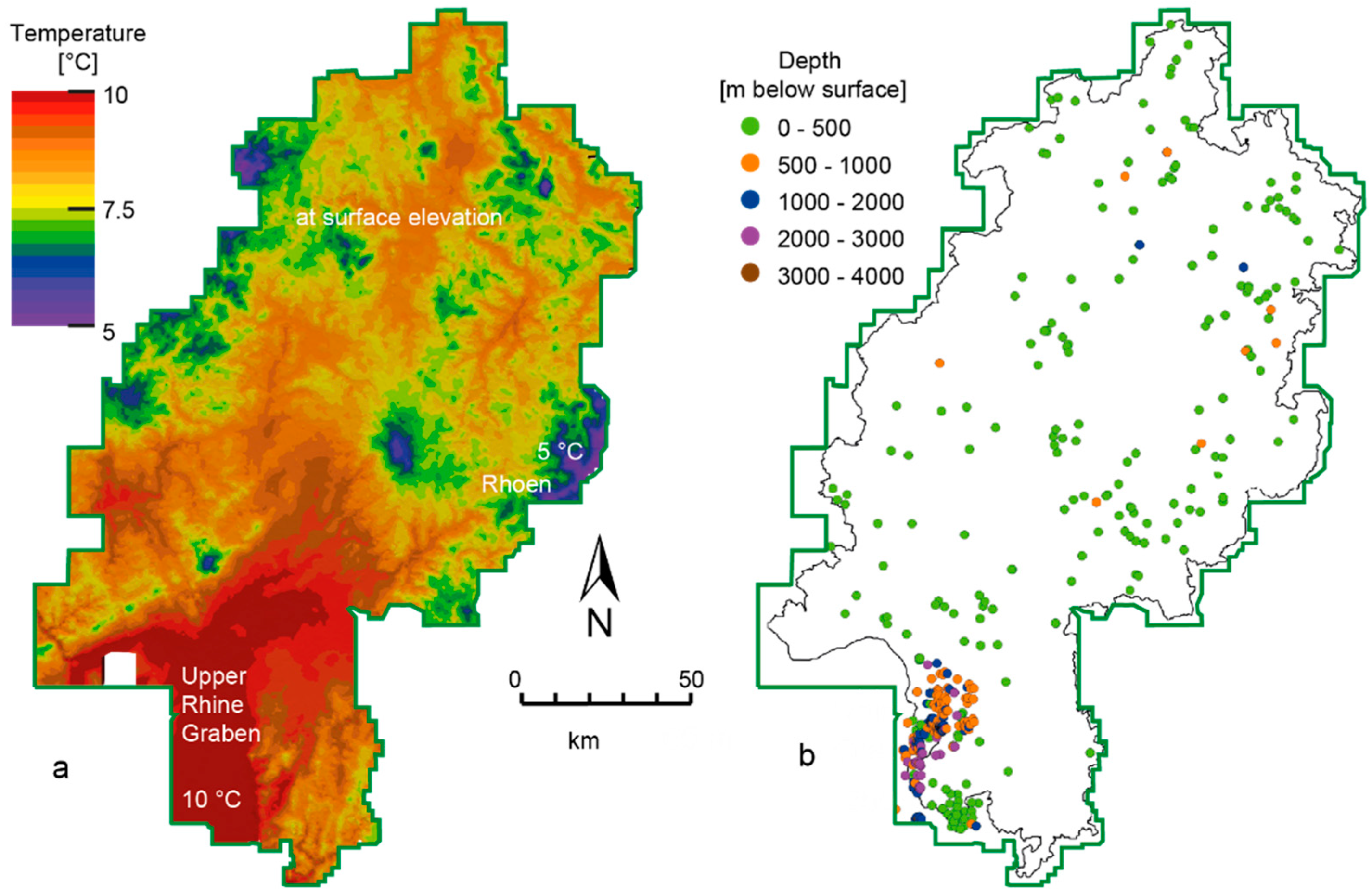
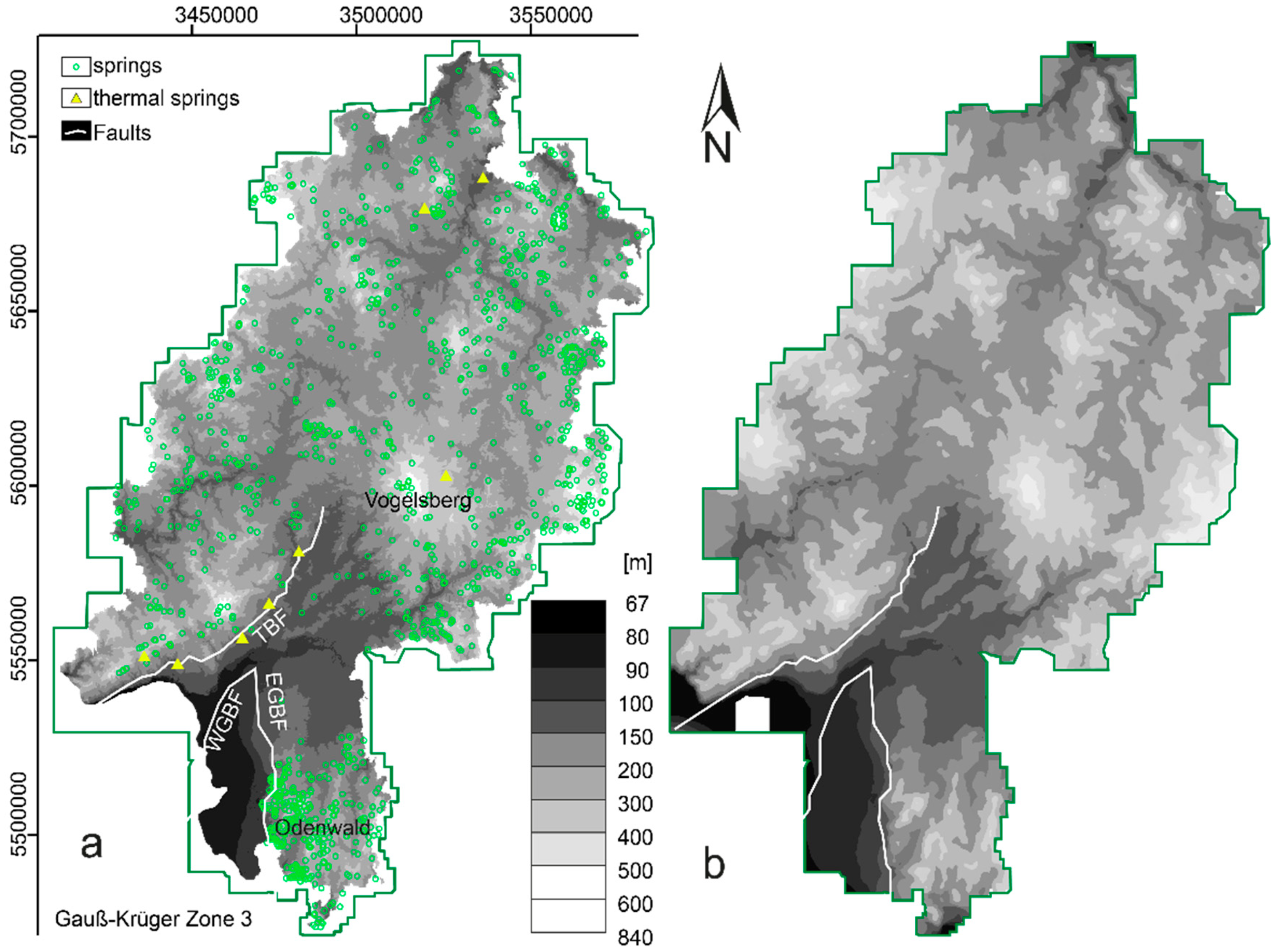
  • Areas where the deep thermal field is mainly controlled by conductive heat transport are identified in North-West Hesse (Rhenish Massif), in East Hesse (Rhoen) and in South-East Hesse (Odenwald). There, measured temperatures are well reproduced assuming steady-state conductive heat transport. This implies that the distribution of heat conductivity and radiogenic heat production are well chosen in the parameterization. In these regions, the permeability is low and thus fluid flow related heat transport is negligible.
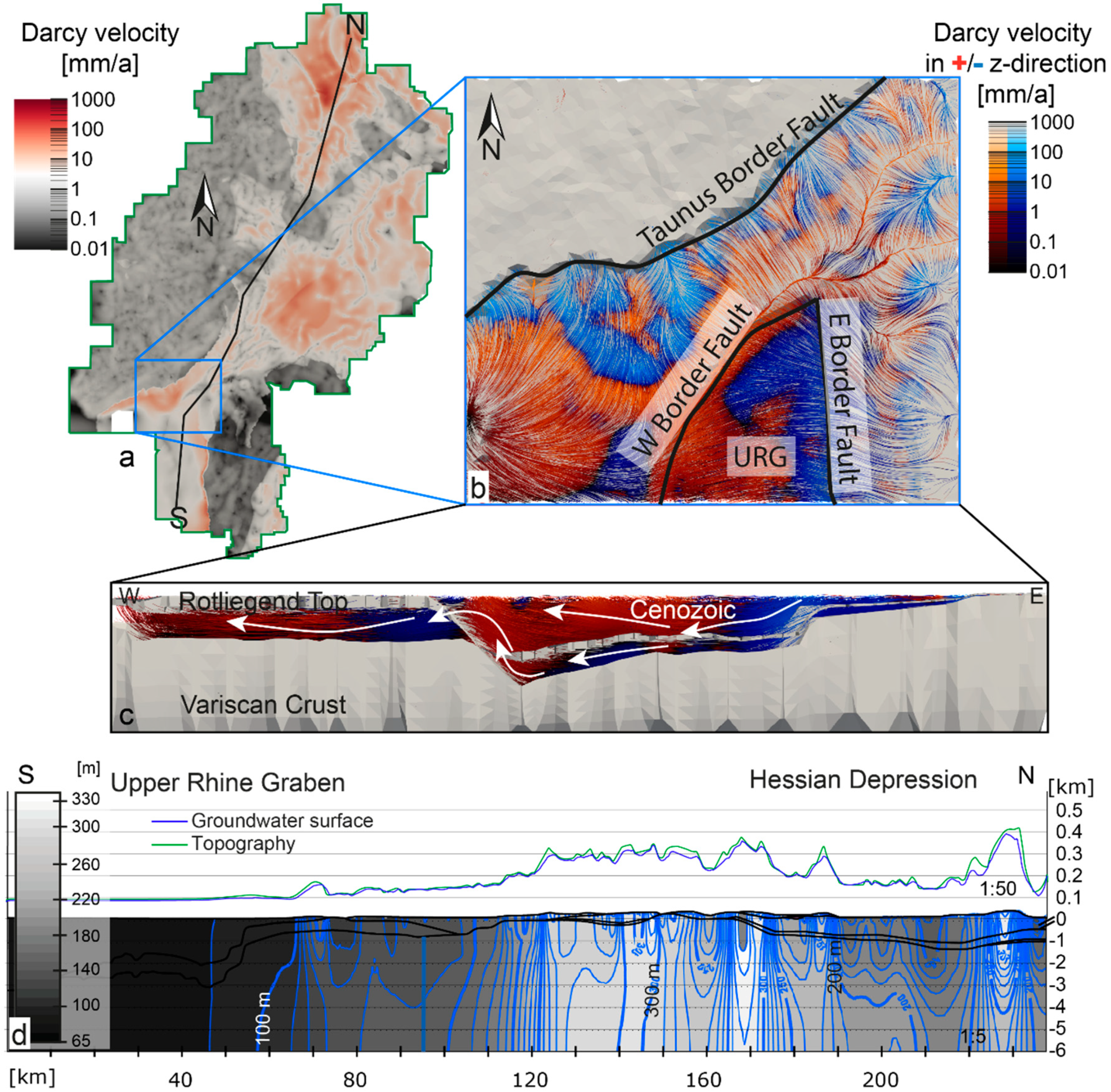
  • Areas additionally influenced by pressure-driven fluid flow are North Hesse (Hessian Depression), central Hesse (Vogelsberg) and South Hesse (Eastern Graben Fault of Upper Rhine Graben). A regional flow field evolves in response to the structural and hydraulic configuration of the subsurface. At the Eastern Graben Fault, this flow field is induced by high hydraulic pressures at the Graben shoulders in concert with contrasting permeabilities, which are high in the Cenozoic sediments and low in the Variscan crust.
  • Local domains are identified where density driven fluid flow can evolve and can overprint the effects of conductive and advective heat transport in the Cenozoic sediments of the Upper Rhine Graben. In these areas, a sufficiently thick permeable unit provides the conditions for buoyancy-driven fluid flow and thus free convective heat transport.
  • Building on this regional differentiation of domains controlled by different heat transport mechanisms, future work should focus on the domains of pressure driven and free convection. Local higher resolved models, taking e.g., faults and facies dependent parameterization into account, could address the prediction of exact temperatures and flow conditions.

Supplementary Materials

Supplementary Material S1: https://www.mdpi.com/1996-1073/12/11/2081/s1, Figure S1: thickness maps; Supplementary Material S2: https://www.mdpi.com/1996-1073/12/11/2081/s2, Governing equations for fluid and heat transport solved in FEFLOW®.

Author Contributions

N.K.: conceptualization and modelling as well as writing—original draft preparation M.S.-W. and I.S.: project administration, M.S.-W., J.B. and M.C.: supervision, J.B. and K.B. funding acquisition, M.F. helped with software, modelling and visualization, J.-G.F. provided data from HLNUG and helped with hydraulic results, All authors were responsible for editing and reviewing the manuscript.

Funding

The Federal Ministry for Economic Affairs and Energy (BMWi) is gratefully acknowledged for economic support through the research project “Hessen-3D II: 3D-Modellierung der geothermischen Tiefenpotenziale von Hessen”, coordinated by the Technical University of Darmstadt (grant agreement no. 0325944 A and 0325944 B).

Acknowledgments

We kindly acknowledge DHI WASY for the sponsored MIKE Powered by DHI license files. Furthermore, we are thankful for all provided data by the HLNUG. We want to thank the reviewers for their contributions which helped improve the quality of this manuscript.

Conflicts of Interest

The authors declare no conflict of interest.

Appendix A. Temperature Database Consisting of Measured Temperatures

Surface temperature measurements were provided by the German Meteorological Service [50] averaged over one year 2013 (Figure A1a). The temperatures vary between 5 °C, at high elevations like in the Rhoen in central East Hesse and 10 °C in the Upper Rhine Graben at low topography in South Hesse.
Figure A1. Temperature data; (a) applied Dirichlet boundary conditions for temperature at the top (annual mean temperature, [50]); color code indicates temperature from purple low temperatures to red high temperatures, maxima and minima are declared in white; (b) overview on the spatial distribution of temperature measurements taken from boreholes within different depths. Deepest boreholes are in Cenozoic units in the Upper Rhine Graben.
Energies 12 02081 g0a1
The temperature database used to “constrain” the simulated temperature field at depth consists of 467 boreholes (locations in Figure A1b) reaching different depths (up to 3314 m below surface in the Upper Rhine Graben). These measurements were obtained using different measurement techniques. In 90% of the boreholes, temperature logs were measured, for 9% of the wells bottom hole temperatures are available and 1% of the measurements come from production tests. Most of the bottom hole temperature measurements are located in the Upper Rhine Graben and originate from hydrocarbon exploration boreholes. In total 3642 temperature measurements could be compared to modelled temperatures. Data from 159 borehole data were provided by the Hessian Agency for Nature Conservation, Environment and Geology (HLNUG), 21 by the Technical University of Darmstadt, 60 by the hydrocarbon industry, 61 by the Leibnitz Institute for Applied Geophysics, 138 by ExxonMobile, 27 by the RWE-DEA AG and 1 by the Wintershall Holding GmbH.
In response to petroleum exploration, both the majority and the deepest boreholes are located in the Upper Rhine Graben. In general, a sufficient coverage of temperature measurements was available over the whole model area.

Appendix B. Hydraulic and Hydrochemical Datasets

Appendix B.1. Hydraulic Database

The groundwater surface of the uppermost groundwater horizon usable for drinking water production was assigned as hydraulic upper boundary condition (Figure A2b). It was constructed by Herrmann [18] based on all available groundwater data of Hesse including hydrogeological maps, groundwater isoline maps, soil moisture classes, groundwater measurements, surface water bodies, groundwater bodies and groundwater catchment areas. The resulting groundwater surface is relatively shallow in the Upper Rhine Graben, where the groundwater surface is nearly equal to the topographic surface (65 m above msl). In contrast, the groundwater surface is at higher elevations in topographically high areas. In the Rhoen, for example, the groundwater surface is about 100 m below the surface at 840 m above msl. To additionally validate the hydraulic field of Hesse, the locations of 1562 springs and of eight hot springs (Figure A2a) are compared to the flow regime predicted by the simulations. The largest part of the spring data is available for South-East Hesse in the Odenwald. Most of the thermal springs in Hesse are located along the South Taunus Border Fault. In contrast to the distribution of the temperature data, there was no information available on springs in the Upper Rhine Graben.
Figure A2. (a) Groundwater surface based on the model by Herrmann [18]. Locations of springs (green circles) and thermal springs (yellow triangles) in Hesse (data from HLNUG). (b) Groundwater surface used as the upper hydraulic boundary condition. White lines indicate the surface geometry of the three main faults in the model area.
Energies 12 02081 g0a2

Appendix B.2. Recharge Data

Moreover, data on mean groundwater recharge from two different sources were available (Figure A3). The first recharge model, averaged over 30 years, was provided by Neumann et al. in a 1 × 1 km grid (Figure A3a, [56]). Another dataset was recently published [54] using the soil water balance model GWN-BW [59] over a timeframe spanning from 1951 to 2015 (Figure A3b). This dataset has a horizontal resolution of 100 × 100 m and can be compared with simulated up flow and down flow zones later on in the validation procedure.
Figure A3. Recharge data for the Federal State of Hesse from (a) Neumann et al., [56] and (b) Kopp et al. [54].
Energies 12 02081 g0a3

Appendix B.3. Hydrochemical Observations

Hydrochemical investigations delivered interpretations of potential hydraulic interactions within and across fault zones and geological units. The results from previous studies suggested that the Western Border Fault of the northern Upper Rhine Graben and the Taunus Border Fault (Figure 1b) are likely to be not connected hydraulically [16]. Moreover, these studies suggested that the Taunus border fault is not permeable both for along and across the fault flow, if not over short segments oriented SE-NW and thus parallel to the present-day direction of maximal horizontal stress (SE-NW) [16,57]. In more detail, the WSW-ENE trending Taunus Border Fault is crosscut by younger Cenozoic faults trending NW-SE. Where these cross-cutting faults occur with larger horizontal displacements, thermal springs are located. Isotope investigations of 87Sr/86Sr showed that meteoric water recharges in the Odenwald and ascends at the western border fault as a consequence of topography driven fluid flow [57]. Loges et al. [60] suggested that water ascending along the Taunus border fault is both sourced from the Taunus (southern part of the Rhenish Massive in Hesse) and from the sedimentary graben fill of the Upper Rhine Graben. In addition, Siemon et al. [53] evidenced rising saltwater along the western main border fault of the Upper Rhine Graben based on geomagnetic and geoelectric methods. Finally, several given chemical observations indicated that the Taunus border fault and western border fault of the Upper Rhine Graben are locations of thermal uprising water, with the Rhenish massif in the North and the Odenwald in the East as main recharge areas. Chemical investigations on deep fluid circulations in Hesse were carried out only for the southernmost areas.

Appendix C

The Cenozoic unit combines Quaternary sediments, which are prevailingly gravels and sands and have high hydraulic conductivities of 1 × 10⁻⁴ m/s [18], Tertiary volcanic rocks with a rather low hydraulic conductivity of 7.9 × 10⁻¹⁰ m/s [9] and Tertiary sediments, which are alternating aquifers and aquitards [13,61]. However, given the level of geological differentiation of the structural model, we imposed a simplified hydraulic parameterization of the Cenozoic deposits. As in Stober and Bucher [49], we used 1 × 10⁻⁷ m/s for this heterogeneous layer, which is consistent with the predominant lithology of sands and marls defined by Grimm [62].
During the Muschelkalk, successively limestone, dolomite, gypsum and halite evaporated and the sequence is partly interbedded by clays of the Middle Muschelkalk. From Keuper times onward, clay, dolomite, sandstone and quartzite were deposited [63]. Muschelkalk and Keuper are present only as relicts in Hesse. As a consequence of regional uplift of the whole area lasting from the middle Jurassic until Palaeocene times, the Keuper and Muschelkalk deposits were largely eroded, and local relicts are only preserved in small graben structures [20].
The Buntsandstein unit is characterized by a higher hydrothermal potential [21,64] and is dominated by two lithological groups: sandstones [8,21,65,66] characterized by a relatively high permeability (Table 2) and thick units of sandstones-pelite intercalations acting as aquitards.
In Zechstein times, different carbonate sediments (limestone, dolomite) and evaporitic rocks (successively limestone, dolomite, gypsum, halite and sylvinite) were deposited due to tropical climate conditions. In areas of the very shallow sea, different copper shales and mineral ores developed [63]. Therefore, the Zechstein unit is mainly characterized by very low porosity and permeability [21], acting as an effective aquitard in the simulations (Table 2). The thermal conductivity of the Zechstein unit varies between 0.5 and 5 W/m × K and has thus the highest internal variability of all units [21].
The lowermost sedimentary unit consists of the continental clastic and volcanic deposits of the Rotliegend with very heterogeneous petrology [10,21,67]. Due to diagenetic processes, the Rotliegend unit has a lower hydraulic conductivity than the Buntsandstein and the Cenozoic aquifers (Table 2) but can be still considered as a regional aquifer in the model.
The upper crust is differentiated into SW-NE striking, vertically bounded Variscan crustal domains [8,19,38]. Freymark et al. [8] found that the radiogenic heat production in these domains has to be differentiated to correctly predict the conductive thermal field in Hesse. Hence in this study, this parameter was assigned consistently to Freymark et al. [8] differentiating the Rhenohercynian, Northern Phyllite Zone and Mid German Crystalline High (parameter S in Table 2). Moreover, as explained by Rühaak et al. [23] and Bär [21] the crust cannot be parameterized by a single uniform value for hydraulic conductivity, porosity, thermal conductivity and heat capacity. The Rhenohercynian domain has to be differentiated hydraulically from the Northern Phyllite Zone and the Mid-German Crystalline High as a separate domain (compare Table 1). Following investigations of the uppermost part of the crystalline crust in the Upper Rhine Graben, the transition zone between the crystalline crust and the sediments is weathered and more permeable, thus favoring fluid flow in this domain (e.g., References [3,16]). Other investigations proposed a low permeability of the crystalline crust allowing only diffusive heat transport in this unit (e.g., Reference [48]). To consider these results from earlier studies we assigned the uppermost numerical layer (no. 16) of the Variscan crust a higher hydraulic conductivity after Bär [21] of 1.4 × 10⁻⁹ m/s in the Rhenohercynian and of 2.9 × 10⁻¹⁰ m/s in the Northern Phyllite Zone and the Mid German Crystalline High. For the deeper part of the crystalline crust, the hydraulic conductivity was set to 7.9 × 10⁻¹² m/s (threshold after Clauser et al. [48], Table 2 and Lampe and Person [68]) to inhibit convective heat transport in the deeper Variscan Crust.

References

  1. Clauser, C. Conductive and Convective Heat Flow Components in the Rheingraben and Implications for the Deep Permeability Distribution. In Hydrogeological Regimes and Their Subsurface Thermal Effects; Beck, A.E., Garven, G., Stegena, L., Eds.; American Geophysical Union: Washington, DC, USA, 1989; Volume 47, pp. 59–65. [Google Scholar]
  2. Clauser, C.; Villinger, H. Analysis of conductive and convective heat transfer in a sedimentary basin, demonstrated for the Rheingraben. Geophys. J. Int. 1990, 100, 393–414. [Google Scholar] [CrossRef]
  3. Pribnow, D.; Clauser, C. Heat and fluid flow at the Soultz hot dry rock system in the Rhine Graben. In Proceedings of the World Geothermal Congress 2000, Kyushu, Tohoku, Japan, 28 May–10 June 2000. [Google Scholar]
  4. Bächler, D.; Kohl, T.; Rybach, L. Impact of graben-parallel faults on hydrothermal convection––Rhine Graben case study. Phys. Chem. Earth 2003, 28, 431–441. [Google Scholar] [CrossRef]
  5. Baillieux, P.; Schill, E.; Abdelfettah, Y.; Dezayes, C. Possible natural fluid pathways from gravity pseudo-tomography in the geothermal fields of Northern Alsace (Upper Rhine Graben). Geotherm. Energy 2014, 2, 16. [Google Scholar] [CrossRef] [Green Version]
  6. Vidal, J.; Genter, A. Overview of naturally permeable fractured reservoirs in the central and southern Upper Rhine Graben: Insights from geothermal wells. Geothermics 2018, 74, 57–73. [Google Scholar] [CrossRef]
  7. Freymark, J.; Bott, J.; Cacace, M.; Ziegler, M.; Scheck-Wenderoth, M. Influence of the Main Border Faults on the 3D Hydraulic Field of the Central Upper Rhine Graben. Geofluids 2019, 2019, 21. [Google Scholar] [CrossRef]
  8. Freymark, J.; Sippel, J.; Scheck-Wenderoth, M.; Bär, K.; Stiller, M.; Fritsche, J.-G.; Kracht, M. The deep thermal field of the Upper Rhine Graben. Tectonophysics 2017, 694 (Suppl. C), 114–129. [Google Scholar] [CrossRef]
  9. Bär, K.; Arndt, D.; Fritsche, J.-G.; Götz, A.E.; Kracht, M.; Hoppe, A.; Sass, I. 3D-Modellierung der tiefengeothermischen Potenziale von Hessen—Eingangsdaten und Potenzialausweisung. [3D modelling of the deep geothermal potential of the Federal State of Hesse (Germany)—Input data and identification of potential]. Z. Dtsch. Ges. Geowiss. 2011, 162, 371–388. [Google Scholar] [CrossRef]
  10. Aretz, A.; Bär, K.; Götz, A.; Sass, I. Outcrop analogue study of Permocarboniferous geothermal sandstone reservoir formations (northern Upper Rhine Graben, Germany): Impact of mineral content, depositional environment and diagenesis on petrophysical properties. Int. J. Earth Sci. 2016, 105, 1431–1452. [Google Scholar] [CrossRef]
  11. Schilling, O.; Sheldon, H.A.; Reid, L.B.; Corbel, S. Hydrothermal models of the Perth metropolitan area, Western Australia: Implications for geothermal energy. Hydrogeol. J. 2013, 21, 605–621. [Google Scholar] [CrossRef]
  12. Simms, M.A.; Garven, G. Thermal convection in faulted extensional sedimentary basins: Theoretical results from finite-element modeling. Geofluids 2004, 4, 109–130. [Google Scholar] [CrossRef]
  13. Lampe, C.; Person, M. Advective cooling within sedimentary rift basins—Application to the Upper Rhinegraben (Germany). Mar. Pet. Geol. 2002, 19, 361–375. [Google Scholar] [CrossRef]
  14. Rühaak, W.; Rath, V.; Clauser, C. Detecting thermal anomalies within the Molasse Basin, southern Germany. Hydrogeol. J. 2010, 18, 1897–1915. [Google Scholar] [CrossRef]
  15. Cherubini, Y.; Cacace, M.; Scheck-Wenderoth, M.; Noack, V. Influence of major fault zones on 3-D coupled fluid and heat transport for the Brandenburg region (NE German Basin). Geotherm. Energy Sci. 2014, 2, 1–20. [Google Scholar] [CrossRef]
  16. Kraml, M.; Jodocy, M.; Reinecker, J.; Leible, D.; Freundt, F.; Al Najem, S.; Schmidt, G.; Aeschbach, W.; Isenbeck-Schröter, M. TRACE: Detection of Permeable Deep-Reaching Fault Zone Sections in the Upper Rhine Graben, Germany, During Low-Budget Isotope-Geochemical Surface Exploration. In Proceedings of the European Geothermal Congress 2016, Strasbourg, France, 19–24 September 2016. [Google Scholar]
  17. Person, M.; Raffensperger, J.P.; Ge, S.; Garven, G. Basin-scale hydrogeologic modeling. Rev. Geophys. 1996, 34, 61–87. [Google Scholar] [CrossRef]
  18. Herrmann, F. Entwicklung einer Methodik zur Großräumigen Modellierung von Grundwasserdruckflächen am Beispiel der Grundwasserleiter des Bundeslandes Hessen; Brandenburgische Technische Universität Cottbus: Cottbus, Germany, 2010. [Google Scholar]
  19. Freymark, J.; Sippel, J.; Scheck-Wenderoth, M.; Bär, K.; Stiller, M.; Kracht, M.; Fritsche, J.-G. Heterogeneous Crystalline Crust Controls the Shallow Thermal Field—A Case Study of Hessen (Germany). Energy Procedia 2015, 76, 331–340. [Google Scholar] [CrossRef]
  20. Arndt, D. Geologische Strukturmodellierung von Hessen zur Bestimmung von Geopotenzialen. Ph.D. Thesis, TU Darmstadt, Darmstadt, Germany, 2012. [Google Scholar]
  21. Bär, K. Untersuchung der Tiefengeothermischen Potenziale von Hessen. Ph.D. Thesis, TU Darmstadt, Darmstadt, Germany, 2012. [Google Scholar]
  22. Sass, I.; Hoppe, A.; Arndt, D.; Bär, K. Forschungs-und Entwicklungsprojekt 3D Modell der Geothermischen Tiefenpotenziale von Hessen. Available online: https//www.energieland.hessen.de/pdf/3-D-Modell-Hessen-Endbericht_(PDF,_7.300_KB).pdf (accessed on 2 July 2013).
  23. Rühaak, W.; Bär, K.; Sass, I. Combining Numerical Modeling with Geostatistical Interpolation for an Improved Reservoir Exploration. Energy Procedia 2014, 59, 315–322. [Google Scholar] [CrossRef] [Green Version]
  24. Paul, J. Oolithe und Stromatolithen im Unteren Buntsandstein. In Trias—Eine Ganz Andere Welt, Mitteleuropa im Frühen Erdmittelalter; Hauschke, N., Wilde, V., Eds.; Dr. Friedrich Pfeil Verlag: München, Germany, 1999; pp. 263–270. [Google Scholar]
  25. Berger, J.-P.; Reichenbacher, B.; Becker, D.; Grimm, M.; Grimm, K.; Picot, L.; Storni, A.; Pirkenseer, C.; Derer, C.; Schaefer, A. Paleogeography of the Upper Rhine Graben (URG) and the Swiss Molasse Basin (SMB) from Eocene to Pliocene. Int. J. Earth Sci. 2005, 94, 697–710. [Google Scholar] [CrossRef] [Green Version]
  26. Berger, J.-P.; Reichenbacher, B.; Becker, D.; Grimm, M.; Grimm, K.; Picot, L.; Storni, A.; Pirkenseer, C.; Schaefer, A. Eocene-Pliocene time scale and stratigraphy of the Upper Rhine Graben (URG) and the Swiss Molasse Basin (SMB). Int. J. Earth Sci. 2005, 94, 711–731. [Google Scholar] [CrossRef]
  27. Murawski, H.; Albers, H.J.; Bender, P.; Berners, H.-P.; Dürr, S.; Huckriede, R.; Kauffmann, G.; Kowalczyk, G.; Meiburg, P.; Müller, R.; et al. Regional Tectonic Setting and Geological Structure of the Rhenish Massif. In Plateau Uplift; Fuchs, K., von Gehlen, K., Mälzer, H., Murawski, H., Semmel, A., Eds.; Springer: Berlin/Heidelberg, Germany, 1983; pp. 9–38. [Google Scholar]
  28. Bogaard, P.J.F.; Wörner, G. Petrogenesis of Basanitic to Tholeiitic Volcanic Rocks from the Miocene Vogelsberg, Central Germany. J. Petrol. 2003, 44, 569–602. [Google Scholar] [CrossRef] [Green Version]
  29. Jung, S. The Role of Crustal Contamination During the Evolution of Continental Rift-Related Basalts: A Case Study from the Vogelsberg Area (Central Germany). GeoLines 1999, 9, 48–58. [Google Scholar]
  30. Sherwood, G.J. A paleomagnetic and rock magnetic study of Tertiary volcanics from the Vogelsberg (Germany). Phys. Earth Planet. Int. 1990, 62, 32–45. [Google Scholar] [CrossRef]
  31. Dèzes, P.; Schmid, S.M.; Ziegler, P.A. Evolution of the European Cenozoic Rift System: Interaction of the Alpine and Pyrenean orogens with their foreland lithosphere. Tectonophysics 2004, 389, 1–33. [Google Scholar] [CrossRef]
  32. Arndt, D.; Bär, K.; Fritsche, J.-G.; Kracht, M.; Sass, I.; Hoppe, A. 3D structural model of the Federal State of Hesse (Germany) for geopotential evaluation. [Geologisches 3D-Modell von Hessen zur Bestimmung von Geo-Potenzialen.]. Z. Dtsch. Ges. Geowiss. 2011, 162, 353–369. [Google Scholar] [CrossRef]
  33. Paradigm. GOCAD 2009.1 User Guide Part IV Foundation Modeling; Paradigm Holding LLC: Nashville, TN, USA, 2009. [Google Scholar]
  34. HLUG. Geologische Übersichtskarte von Hessen 1:300 000. In 5. Überarbeitete Digitale Ausgabe; HLUG: Wiesbaden, Germany, 2007. [Google Scholar]
  35. Zitzmann, A. Tektonische Karte der Bundesrepublik Deutschland 1:1.000.000; BGR: Hannover, Germany, 1981. [Google Scholar]
  36. Anderle, H.J. Block Tectonic Interrelations between Northern Upper Rhine Graben and Southern Taunus Mountains. In Approaches to Taphrogenesis; Schweizerbart: Stuttgart, Germany, 1974; pp. 243–253. [Google Scholar]
  37. Derer, C.E. Tectono-Sedimentary Evolution of the Northern Upper Rhine Graben (Germany), with Special Regard to the Early Syn-Rift Stage. Ph.D. Thesis, University Bonn, Bonn, Germany, 2003. [Google Scholar]
  38. Franke, W. The mid-European segment of the Variscides: Tectonostratigraphic units, terrane boundaries and plate tectonic evolution. Geol. Soc. Lond. Spec. Publ. 2000, 179, 35–61. [Google Scholar] [CrossRef]
  39. Kossmat, F. Gliederung des varistischen Gebirgsbaues. Abh. Sächsisches Geol. Landesamt 1927, 1, 39. [Google Scholar]
  40. Klügel, T. Geometrie und Kinematik einer variszischen Plattengrenze—Der Südrand des Rhenoherzynikums im Taunus. Geol. Abh. Hess. 1997, 101, 215. [Google Scholar]
  41. Stein, E. The geology of the Odenwald Crystalline Complex. Mineral. Petrol. 2001, 72, 7–28. [Google Scholar] [CrossRef]
  42. Agemar, T.; Alten, J.-A.; Ganz, B.; Kuder, J.; Kühne, K.; Schumacher, S.; Schulz, R. The Geothermal Information System for Germany—GeotIS. Z. Dtsch. Ges. Geowiss. 2014, 165, 129–144. [Google Scholar] [CrossRef]
  43. Agemar, T.; Schellschmidt, R.; Schulz, R. Subsurface temperature distribution in Germany. Geothermics 2012, 44, 65–77. [Google Scholar] [CrossRef]
  44. Agemar, T.; Schellschmidt, R.; Schulz, R. 3D-Modell der Untergrundtemperatur von Deutschland. In Proceedings of the Des Geothermiekongresses 2011 Bochum, Bochum, Germany, 15–17 November 2011. [Google Scholar]
  45. Friedland, G. 3D Modelling of Deep Fluid Flow in the Central Upper Rhine Graben with Respect to Hydraulic Boundary Conditions. Master’s Thesis, Freie Universität Berlin, Berlin, Germany, 2018, unpublished. [Google Scholar]
  46. Diersch, H.-J. FEFLOW—Finite Element Modeling of Flow, Mass and Heat Transport in Porous and Fractured Media, 1st ed.; Springer: Berlin/Heidelberg, Germany, 2014. [Google Scholar]
  47. Kaiser, B.O.; Cacace, M.; Scheck-Wenderoth, M. 3D coupled fluid and heat transport simulations of the Northeast German Basin and their sensitivity to the spatial discretization: Different sensitivities for different mechanisms of heat transport. Environ. Earth Sci. 2013, 70, 3643–3659. [Google Scholar] [CrossRef]
  48. Clauser, C.; Griesshaber, E.; Neugebauer, H.J. Decoupled thermal and mantle helium anomalies: Implications for the transport regime in continental rift zones. J. Geophys. Res. Solid Earth 2002, 107, 2269. [Google Scholar] [CrossRef]
  49. Stober, I.; Bucher, K. Hydraulic conductivity of fractured upper crust: Insights from hydraulic tests in boreholes and fluid-rock interaction in crystalline basement rocks. Geofluids 2015, 15, 161–178. [Google Scholar] [CrossRef]
  50. DWD. Available online: https://werdis.dwd.de (accessed on 2 July 2013).
  51. Cacace, M.; Kaiser, B.O.; Lewerenz, B.; Scheck-Wenderoth, M. Geothermal energy in sedimentary basins: What we can learn from regional numerical models. Chem. Erde Geochem. 2010, 70, 33–46. [Google Scholar] [CrossRef]
  52. Kaiser, B.O.; Cacace, M.; Scheck-Wenderoth, M.; Lewerenz, B. Characterization of main heat transport processes in the Northeast German Basin: Constraints from 3-D numerical models. Geochem. Geophys. Geosyst. 2011, 12. [Google Scholar] [CrossRef]
  53. Siemon, B.; Blum, R.; Pöschl, W.; Voß, W. Aeroelektromagnetische und gleichstromgeoelektrische Erkundung eines Salzwasservorkommens im Hessischen Ried. Geol. Jahrb. Hess. 2001, 128, 115–125. [Google Scholar]
  54. Kopp, B.; Baumeister, C.; Gudera, T.; Hergesell, M.; Kampf, J.; Morhard, A.; Neumann, J. Entwicklung von Bodenwasserhaushalt und Grundwasserneubildung in Baden-Württemberg, Bayern, Rheinland-Pfalz und Hessen von 1951 bis 2015. Hydrol. Wasserbewirtsch. 2018, 62, 62–76. [Google Scholar]
  55. Leßmann, B. Hydrochemische und isotopenhydrologische Untersuchungen an Grundwässern aus dem Vulkangebiet Vogelsberg. Grundwasser 2001, 6, 81–85. [Google Scholar] [CrossRef]
  56. Neumann, J.; Wycisk, P. Mittlere Jährliche Grundwasserneubildung; Bundesministerium für Umwelt, Naturschutz und Reaktorsicherheit: Bonn, Germany, 2003. [Google Scholar]
  57. Kraml, M.; Jodocy, M.; Grobe, R.; GmbH, G.E. Verbundprojekt TRACE—TiefenReservoir-Analyse Und Charakterisierung von Der Erdoberfläche: Teil 1: Bestimmung Chemischer Und Isotopischer Parameter von Fluiden Und Gasen Zur Fündigkeitsabschätzung Und Ihre Anwendbarkeit Auf Tiefengeothermie-Projekte: Schlussbericht Teilvorhaben A: GeoThermal Engineering GmbH: Laufzeit Des Vorhabens: 1.6.2012-31.5.2015. Technical report; GeoThermal Engineering GmbH (GeoT): Karlsruhe, Germany, 2015. [Google Scholar]
  58. Scheck-Wenderoth, M.; Koltzer, N.; Cacace, M.; Bott, J. Regional hydraulic model of the Upper Rhine Graben. Geophys. Res. Abstr. 2019, 21. EGU2019–19216. [Google Scholar]
  59. Morhard, A. Kurzbeschreibung des Modells GWN-BW Erweiterungen in Version 2.0. Stand 13.05.2009 (ergänzt: Mai 2011); GIT HydroS Consult GmbH: Freiburg im Breisgau, Germany, 2009. [Google Scholar]
  60. Loges, A.; Wagner, T.; Kirnbauer, T.; Göb, S.; Bau, M.; Berner, Z.; Markl, G. Source and origin of active and fossil thermal spring systems, northern Upper Rhine Graben, Germany. Appl. Geochem. 2012, 27, 1153–1169. [Google Scholar] [CrossRef]
  61. Stober, I.; Bucher, K. Hydraulic and hydrochemical properties of deep sedimentary reservoirs of the Upper Rhine Graben, Europe. Geofluids 2015, 15, 464–482. [Google Scholar] [CrossRef]
  62. Grimm, K.I. Stratigraphie von Deutschland IX—Tertiär, Teil 1: Oberrheingraben und Benachbarte Tertiärgebiete; Schweizerbart: Stuttgart, Germany, 2011; Volume 75, p. 461. [Google Scholar]
  63. Lotz, K. Einführung in Die Geologie des Landes Hessen; Hitzeroth: Marburg, Germany, 1995; p. 267. [Google Scholar]
  64. Jodocy, M.; Stober, I. Porositäten und Permeabilitäten im Oberrheingraben und Südwestdeutschen Molassebecken. Erdöl Erdgas Kohle 2011, 127, 20–27. [Google Scholar]
  65. GeORG-Projektteam. Geopotenziale des tieferen Untergrundes im Oberrheingraben, Fachlich-Technischer Abschlussbericht des INTERREG-Projekts GeORG, Teil 2: Geologische Ergebnisse und Nutzungsmöglichkeiten; EU-Projekt GeORG, 2013; p. 346. [Google Scholar]
  66. Clauser, C.; Koch, A.; Hartmann, A.; Jorand, R.; Mottaghy, D.C.; Pechnig, R.; Rath, V.; Wolf, A. Erstellung statistisch abgesicherter thermischer und hydraulischer Gesteinseigenschaften für den flachen und tiefen Untergrund in Deutschland: Phase 1—Westliche Molasse und nördlich angrenzendes Süddeutsches Schichtstufenland; Endbericht 01.01.2005–31.10.2006; RWTH: Aachen, Germany, 2007. [Google Scholar]
  67. Molenaar, N.; Felder, M.; Bär, K.; Götz, A.E. What classic greywacke (litharenite) can reveal about feldspar diagenesis: An example from Permian Rotliegend sandstone in Hessen, Germany. Sediment. Geol. 2015, 326, 79–93. [Google Scholar] [CrossRef]
  68. Lampe, C.; Person, M. Episodic hydrothermal fluid flow in the Upper Rhinegraben (Germany). J. Geochem. Explor. 2000, 69–70, 37–40. [Google Scholar] [CrossRef]
Figure 1. (a) Position of the model area marked by a green contour, the sediments of the European Cenozoic Rift System (ECRS) in yellow and of the North German Basin (NGB) in orange; (b) topographic map of Hesse with high regions of Rhenish Massif, Vogelsberg, Rhoen and Odenwald and thick sedimentary deposits of Hessian Depression and Upper Rhine Graben with dashed beige lines. In red, three important main faults at the surface are outlined (modified after Arntd et al. [32]).
Energies 12 02081 g001
Figure 2. Structural 3D model of Hesse: (a) Consisting of six lithological layers and faults (modified after Reference [20]); in this figure the layer surfaces are represented with different colors for each unit and in (b) the depth of the top of the Variscan crust is illustrated in a 3D view with colors from blue to red. The model base in 6 km depth is illustrated as a blue plane. The Variscan crust is subdivided into different Variscan domains (see Figure 1). The vertical borders between the different crustal units are approximated as vertical and illustrated as blue lines [21].
Energies 12 02081 g002
Figure 3. Hydraulic and thermal processes are tested successively with different orders of complexity. Beginning with uncoupled steady-state settings coming to fully coupled transient conditions. Arrows indicate initial conditions (IC) for the next scenario.
Energies 12 02081 g003
Figure 4. Dirichlet boundary condition at the bottom at a 6 km depth (simulated temperatures after Freymark et al. [8]).
Energies 12 02081 g004
Figure 5. Hydraulic field of Hesse simulated under steady-state conditions, (a) map at a 1 km depth showing the simulated Darcy velocities, (b) a zoomed view of the northernmost part of the Upper Rhine Graben with the location of the western and eastern main border faults and the Taunus border fault; color-coded streamlines showing the fluid movement (red upwards and blue downwards), (c) west-east profile cutting through the Upper Rhine Graben, (d) south-north profile (geology shown in Figure 6b), showing isolines of hydraulic heads from white high to black low values.
Energies 12 02081 g005
Figure 6. Conductive thermal configuration. (a) temperature map at a 1 km depth and (b) a geological profile from south to north. The blue line in the profile depicts the border of the crustal Variscan domains, (c) simulated temperatures along this profile.
Energies 12 02081 g006
Figure 7. Depth of the 100 °C isotherm of (a) the conductive steady-state heat transport simulation and (b) the thermo-hydraulic steady-state simulation. The transparent blue block indicates the model domain in three dimensions. The results are shown with ten times vertical exaggeration.
Energies 12 02081 g007
Figure 8. The thermo-hydraulic steady-state configuration from an aerial view and along the south–north profile. (a,b) maps of temperature distribution and Darcy velocity at 1 km depth, (c) Darcy velocity in the z-direction; streamlines in the sediments with red colors indicated as upflow and with blue colors indicated as downflow. (d) south–north profile along the black line in figure (a–c). Geological units in black lines, the background colors illustrate the temperature and grey to white lines show hydraulic head isolines.
Energies 12 02081 g008
Figure 9. Maps of Darcy velocities in mm per year at 1 km depth. (ac) results of coupled thermo-hydraulic simulations with constant viscosity and density after (a) 10,000, (b) 50,000 and (c) 100,000 years. (df) results of coupled thermo-hydraulic simulations with temperature and pressure dependent varying viscosity and density after (d) 10,000, (e) 50,000 and (f) 100,000 years.
Energies 12 02081 g009
Figure 10. Maps of temperature at 1 km depth. (ac) results of coupled thermo-hydraulic simulations with constant viscosity and density after (a) 10,000, (b) 50,000 and (c) 100,000 years. (df) results of coupled thermo-hydraulic simulations with temperature and pressure dependent varying viscosity and density after (d) 10,000, (e) 50,000 and (f) 100,000 years. The south-western model area is shown in (gi) in a zoomed view with different color scales, to better identify the temperatures in the thermal anomalies.
Energies 12 02081 g010
Figure 11. 3D visualization of simulated streamlines in a transient state after 100,000 years of simulation time. The color code shows in red Darcy velocities in the positive z-direction (upflow) and in blue in the negative z-direction (downflow). With velocities from black over dark colors to light colors into white. (a) Streamlines above the Variscan crust in a block in South-West Hesse, (b) profile perpendicular to the Upper Rhine Graben with streamlines in Cenozoic and Rotliegend sediments. White arrows highlight the simulated fluid circulation in the Upper Rhine Graben.
Energies 12 02081 g011
Figure 12. The Federal State of Hesse is subdivided into areas of different characteristic types of heat transport mechanisms; conduction in red, advection in blue and convection in white.
Energies 12 02081 g012
Figure 13. Simulated temperature distribution at 1 km depth with yellow cold to red hot temperatures. Previous modelling studies chronologically by (a) Bär [21], (b) Rühaak et al. [23], (c) Freymark et al. [19] and (d) Freymark et al. [8] and simulation results of this study considering (e) conductive, (f) conductive and advective and (g) conductive, advective and free convective heat transport. (h) illustrates a zoom into the northern part of the Upper Rhine Graben (grey frame in Figure g) to better visualize the single thermal anomalies.
Energies 12 02081 g013
Figure 14. Differences between temperature measurements and temperatures predicted by the thermo-hydraulic model considering conductive, advective and free convective heat transport processes with variable density and viscosity of the fluid. Red spheres represent misfit of more than 20 °C higher simulated temperatures than measured and blue spheres represent misfit of more than 20 °C colder simulated temperatures. White colors indicate a good consistency between measured and simulated temperatures. The depth to the top of the Variscan crust is indicated by isolines and colors in the background.
Energies 12 02081 g014
Figure 15. Streamlines of the vertical component of the fluid flow averaged over the entire model domain of the simulation of the advective thermo-hydraulic steady-state processes. Results show in red ascending and in blue descending groundwater. The lightness of the blue and red colors indicates the Darcy velocities. Location of three faults in white: TBF = Taunus Border Fault, WGBF = Western Graben Border Fault and EGBF = Eastern Graben Border Fault. Green circles are locations of springs and yellow triangles are locations of hot springs.
Energies 12 02081 g015
Table 1. Four existing thermal models use different methods to calculate the thermal field of Hesse.
AuthorArndt et al. [32], Bär [21], Arndt [20]Rühaak et al. [23]Freymark et al. [8,19]Agemar et al. [42,43,44]
MethodInterpolation of measured temperatures in combination with Moho-depth related geothermal gradientsCombined geostochastic interpolation and conductive model to reach the best fit with measurements Simulating physical processes of conductive heat transport in Hesse and the whole Upper Rhine GrabenInterpolation of measured temperatures of Germany’s sedimentary basins (Upper Rhine Graben in Hesse)
Model depth6 km depth6 km depthlithosphere–asthenosphere boundaryvariable depending on measurement depth
Table 2. Physical properties used for all simulations together with a schematic representation of the six geological units. Values were taken from the following literature: (1) Bär et al. [9], (2) Freymark et al. [8], (3) Rühaak et al. [23], (4) Herrmann [18], (5) Clauser et al. [48], (6) Stober and Bucher [49]. K = hydraulic conductivity, n = porosity, λ = thermal conductivity of the solid phase, cs = volumetric heat capacity of the solid, S = radiogenic heat production, RH = Rhenohercynian, NPZ = Northern Phyllite Zone, MGCH = Mid German Crystalline High.
Numerical LayerK [m/s]n [-]λ [W/m × K]cs [MJ/m3K]S [μW/m3]Geological Unit
1–61 × 10−7 (1),(4)0.02 (3)1.84 (3)2.0 (1)0.5 (2)Quarternary/Tertiary
75.7 × 10⁻¹⁰ (1)0.04 (3)2.1 (3)1.8 (1)1.2 (2)Muschelkalk
8, 91.9 × 10⁻⁷ (1)0.14 (3)2.97 (3)1.8 (1)1 (2)Buntsandstein
10, 115.5 × 10⁻⁹ (1)0.12 (3)2.55 (3)2.1 (1)0.8 (2)Zechstein
12–155.5 × 10⁻⁸ (1)0.09 (3)2.42 (3)2.0 (1)1 (2)Rotliegend
16 (6)1.4 × 10⁻⁹ (1)0.04 (3)2.81 (3)1.8 (1)RH: 1 (2)
NPZ: 3 (2)
MGCH: 1.8 (2)
Upper Crust: RH
17–217.9 × 10⁻¹² (5)
16 (6)2.9 × 10⁻¹⁰ (1)0.002 (3)2.4 (3)2.1 (1)Upper Crust: MGCH and NPZ
17–217.9 × 10⁻¹² (5)

