Investigation of Two-Phase Flow in a Hydrophobic Fuel-Cell Micro-Channel


Abstract
1. Introduction
2. Experimental
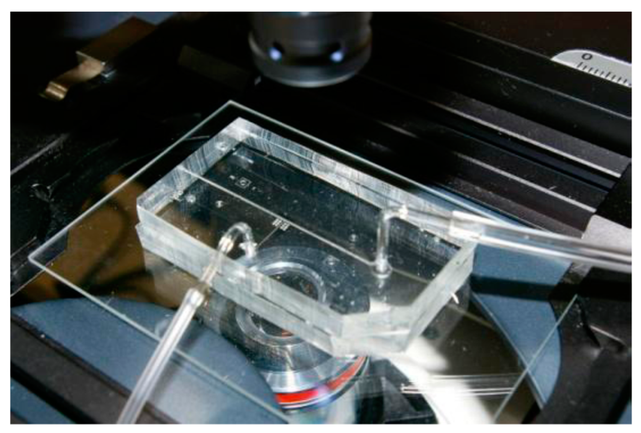
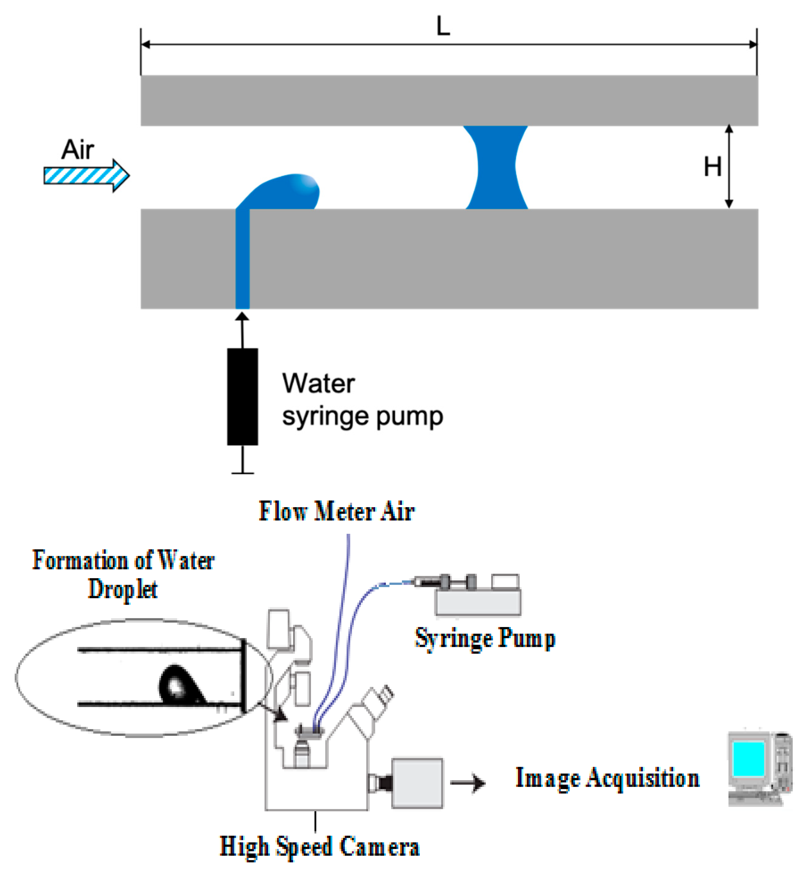
2.1. Microchannel Set-Up and Method
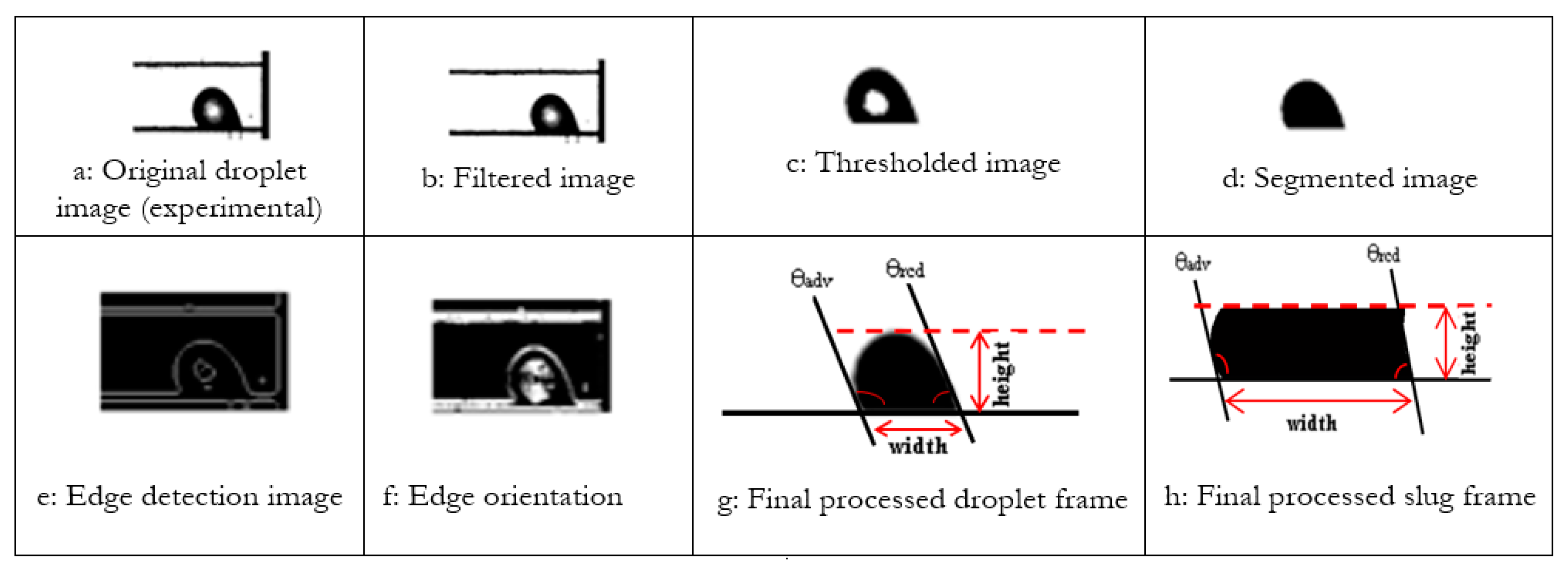
2.2. Image Processing Technique and in-House MATLAB Scripts
3. Liquid Bridge MODEL
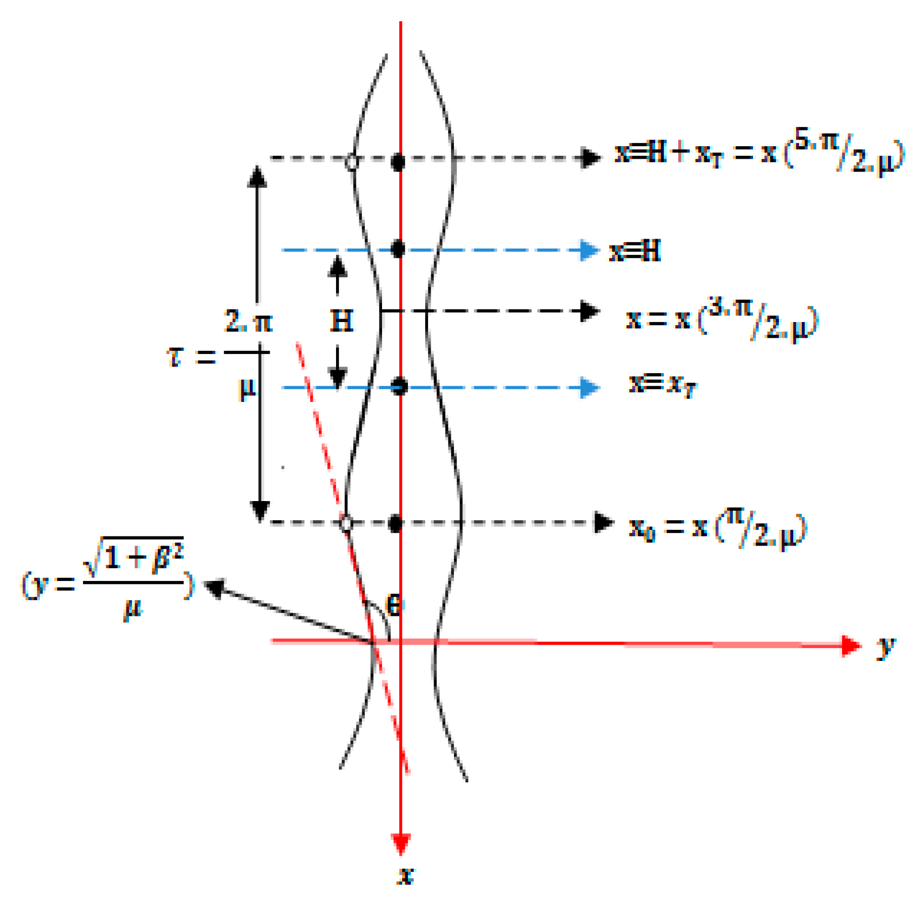
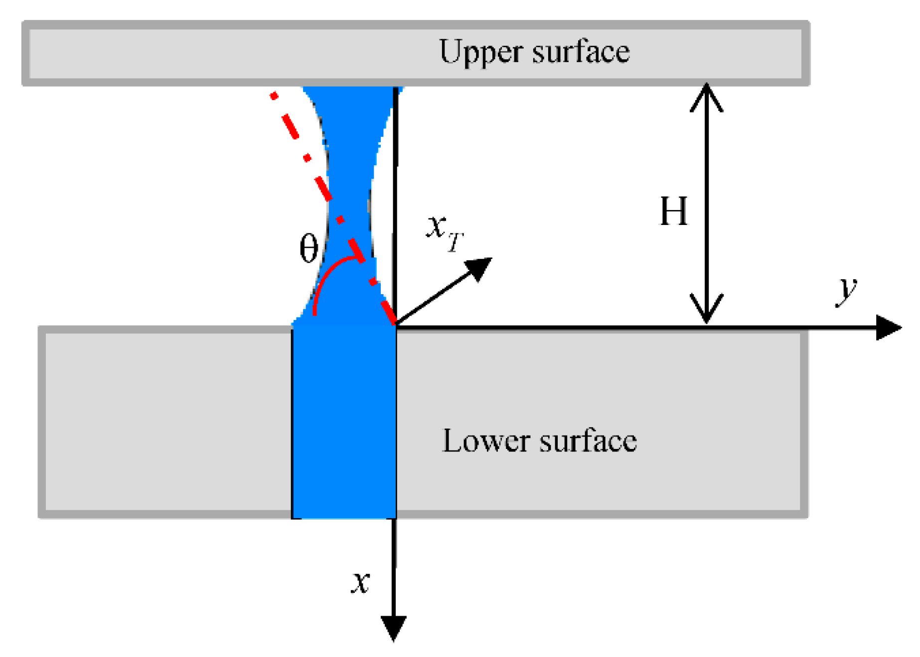
3.1. Formulation
3.2. Numerical Solution
4. Results and Discussion
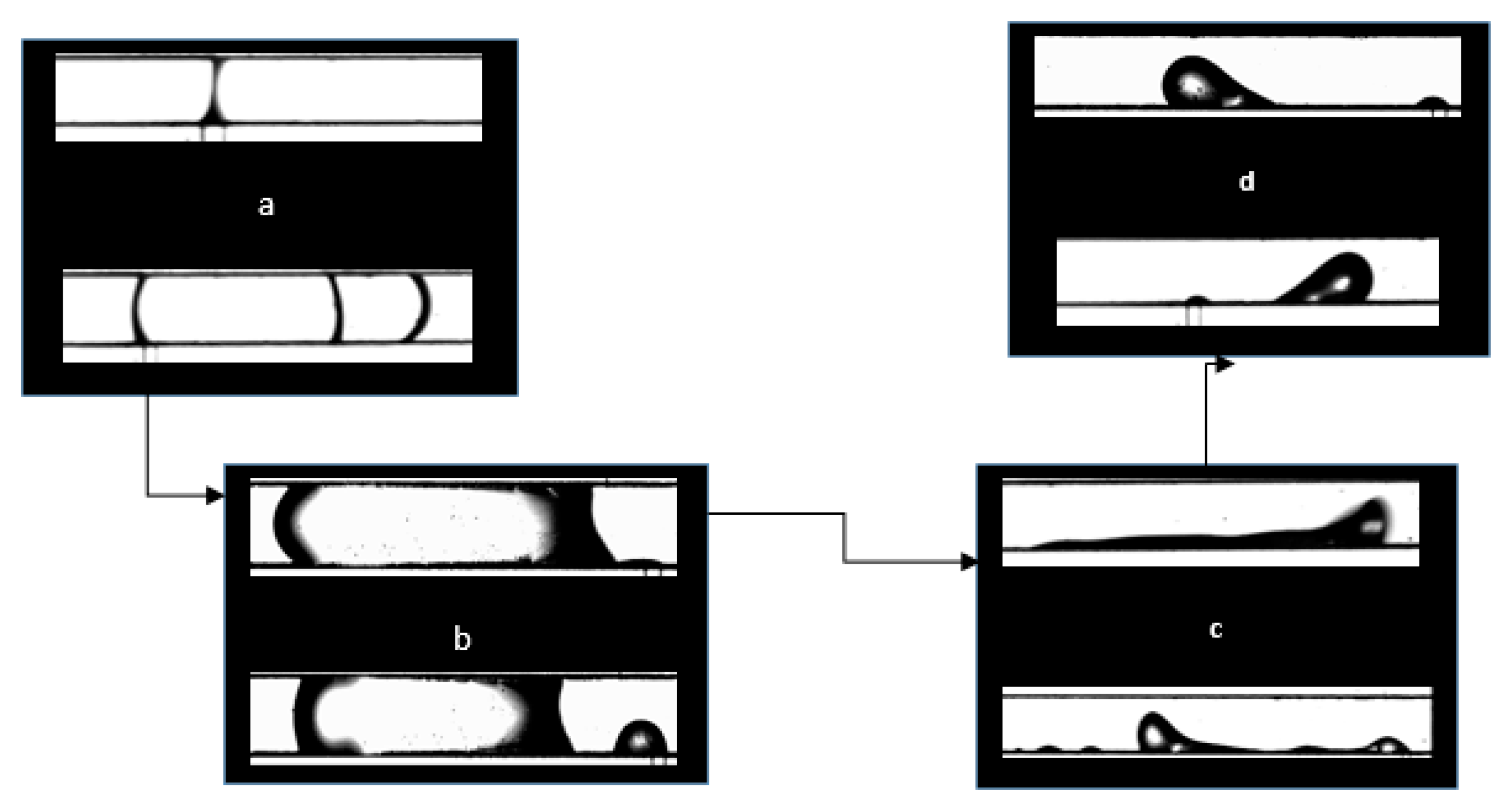
4.1. Flow Patterns
4.1.1. Liquid Bridge/Plug: Relatively Dry Air Conditions ()
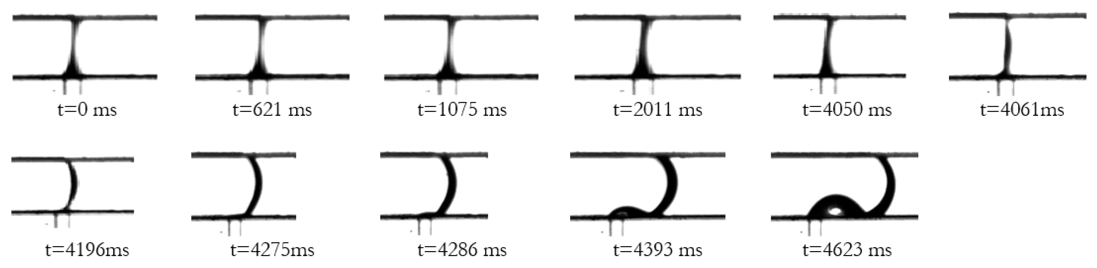
Concave Liquid Bridge/Plug
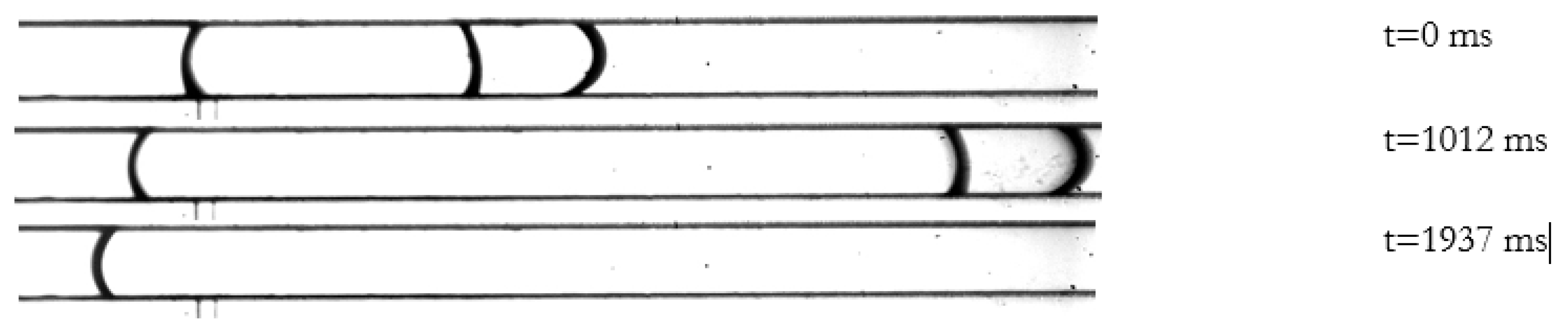
Convex Liquid Bridge/Plug
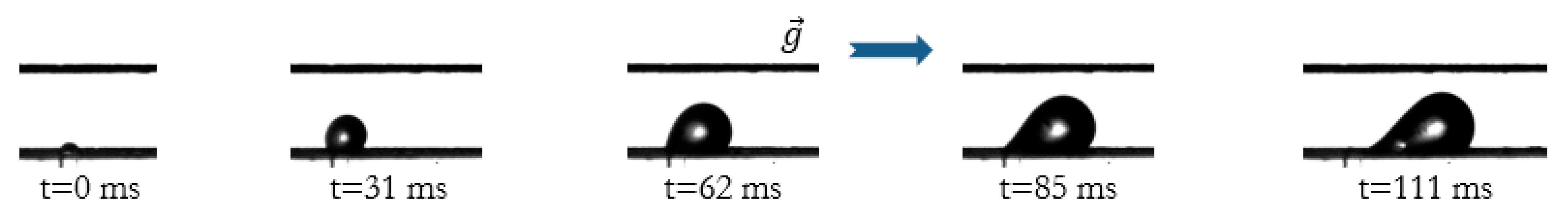
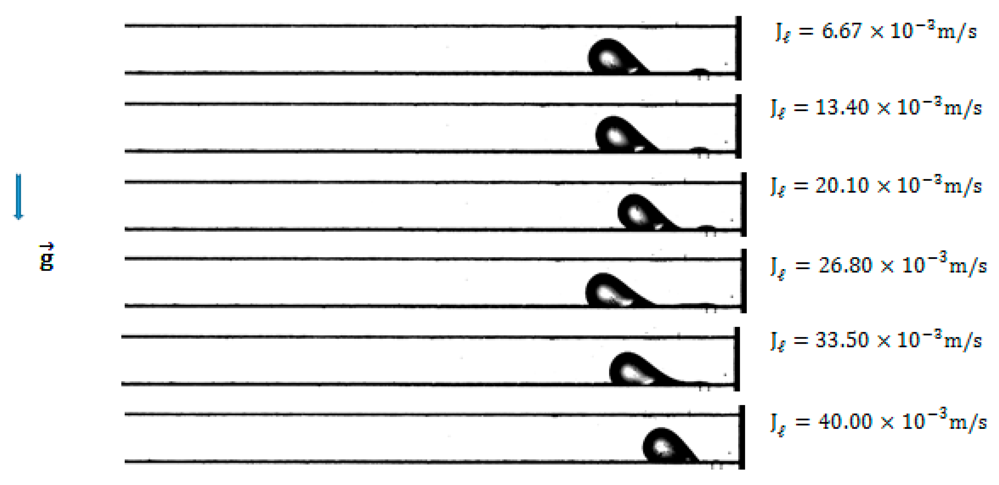
4.1.2. Droplet Flow ()
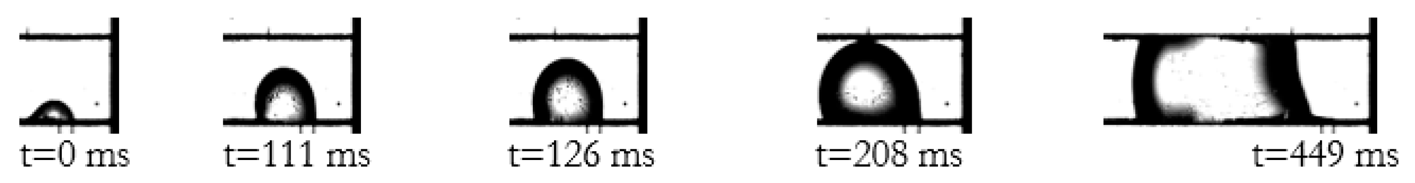
4.1.3. Slug/Plug Flow ()
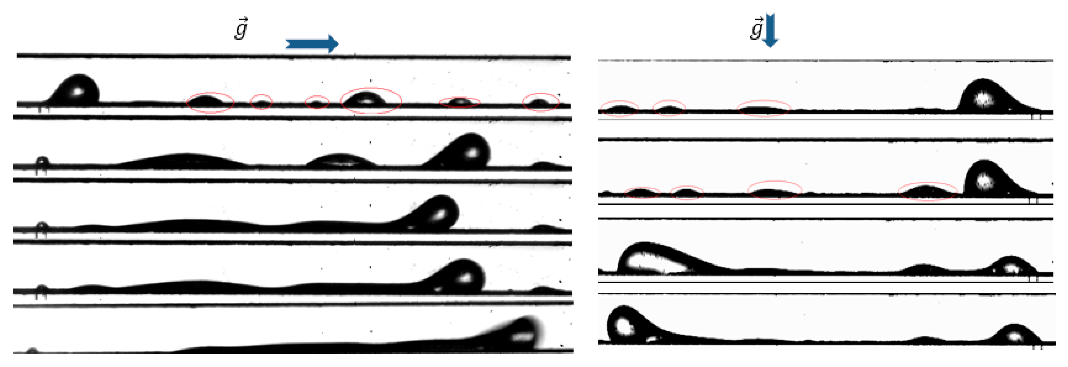
4.1.4. Film Flow
4.2. Droplet and Slug Characteristics
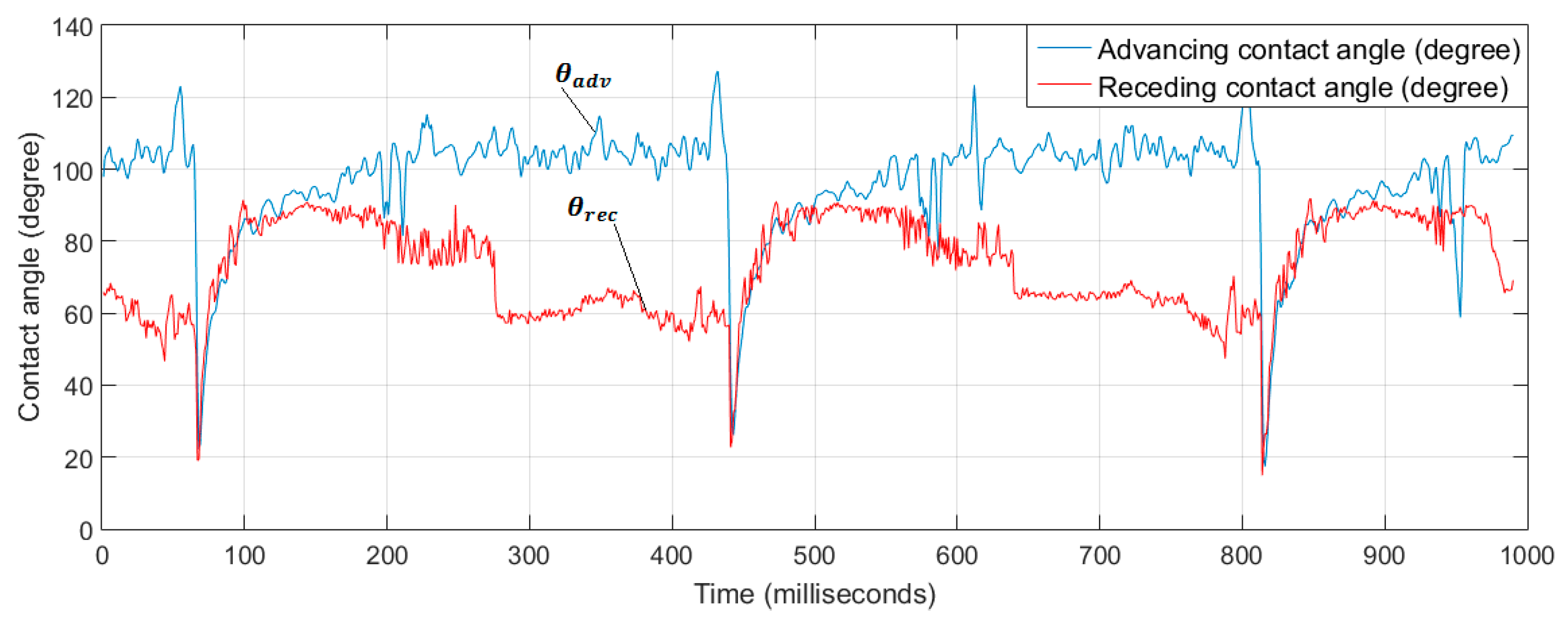
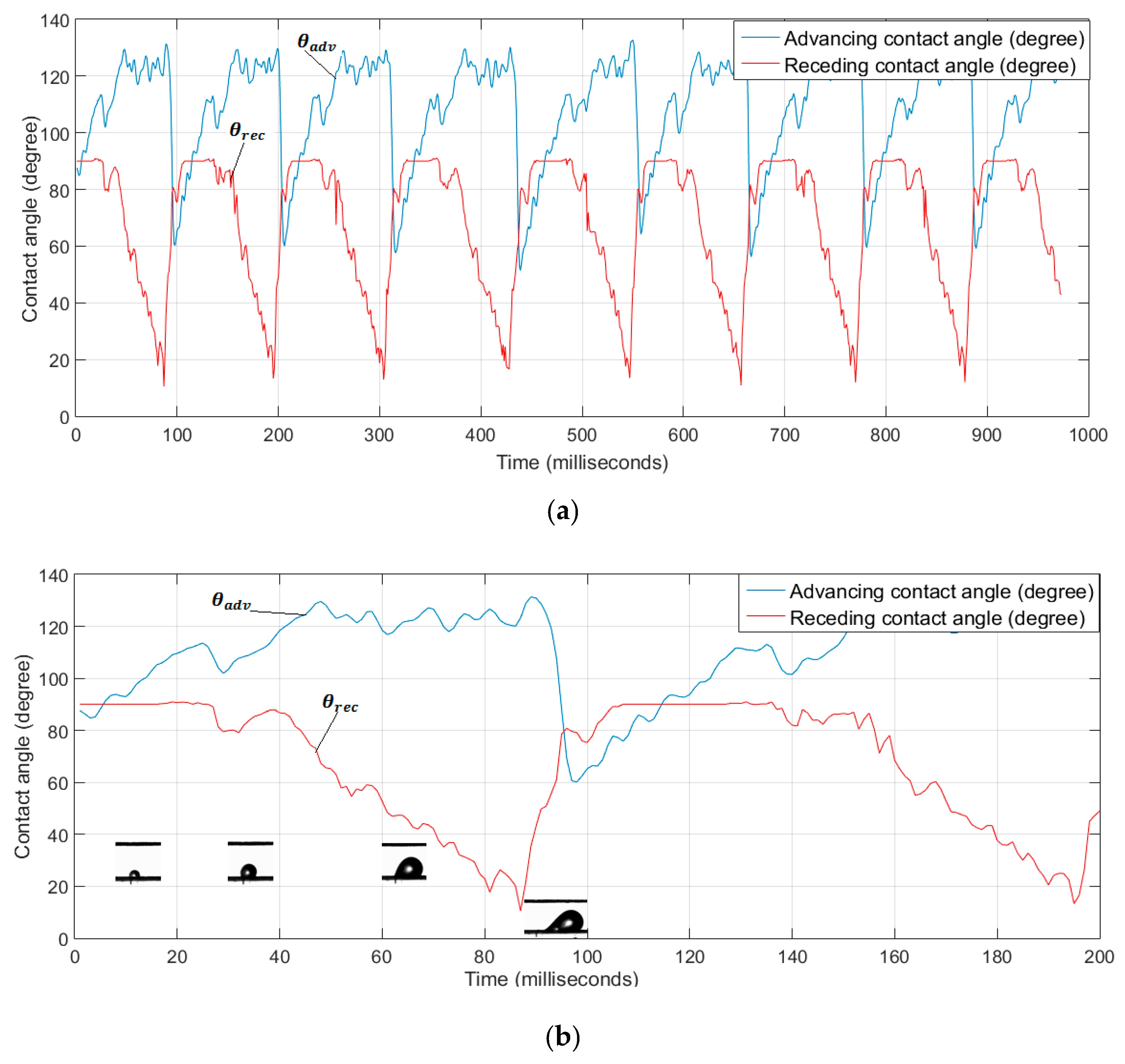
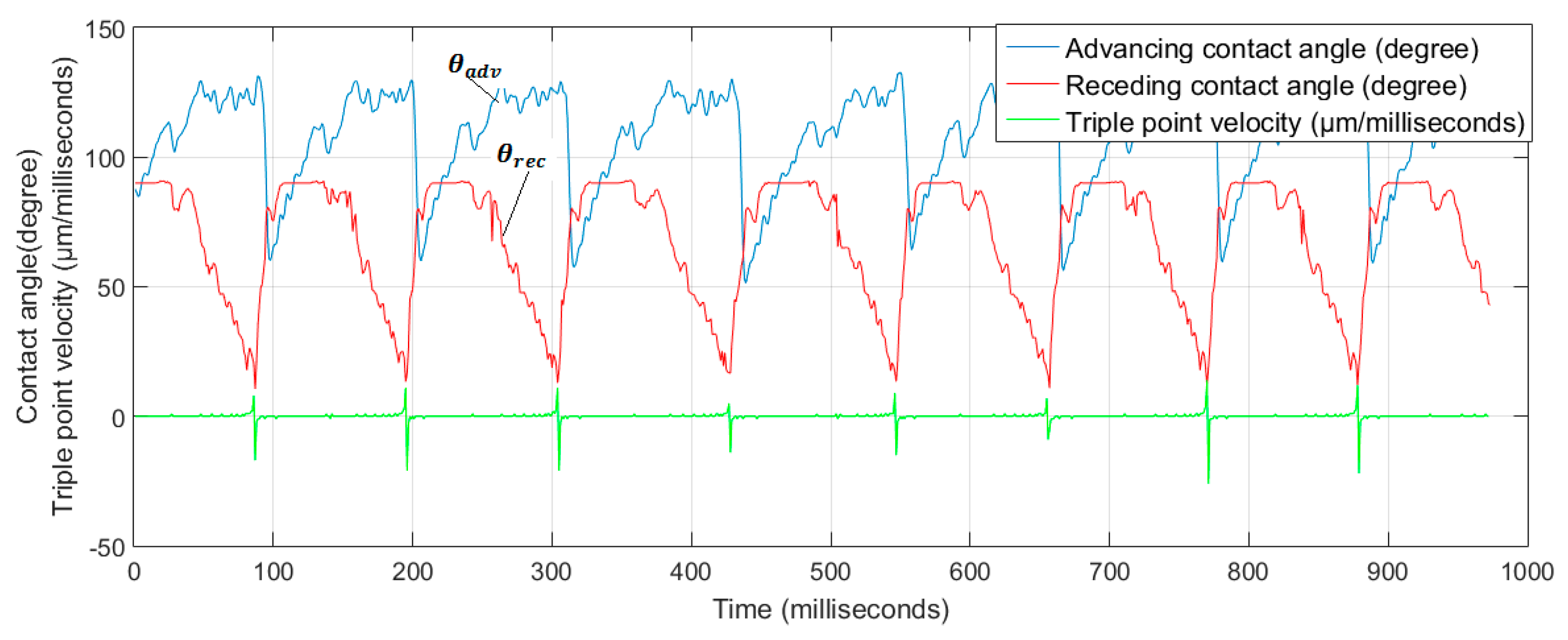
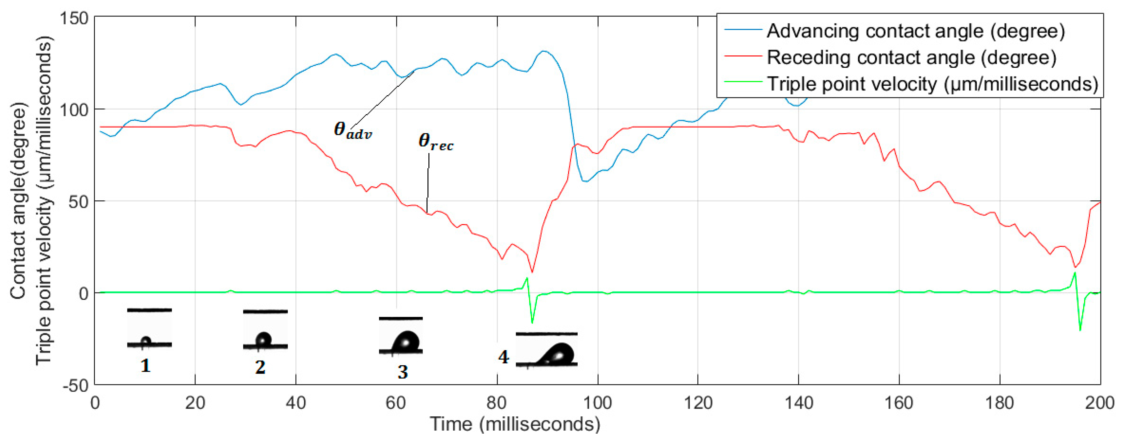
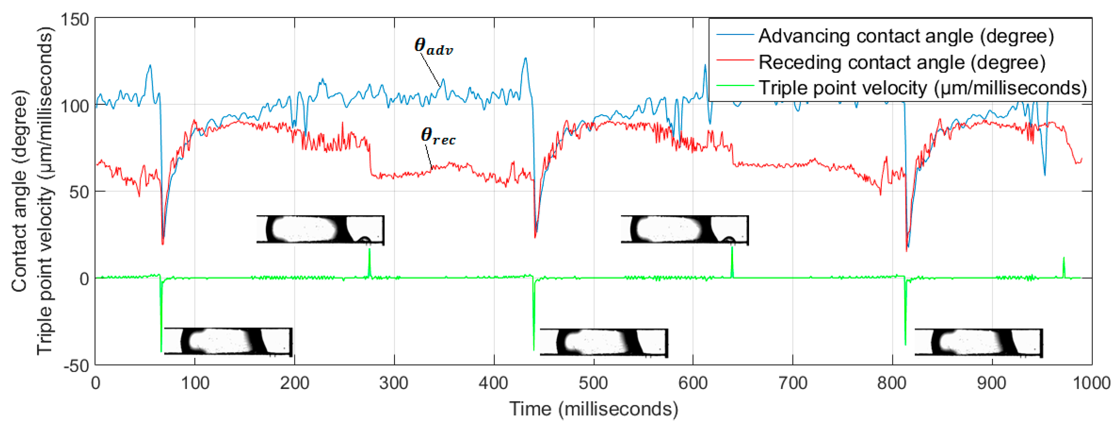
4.2.1. Contact Angles
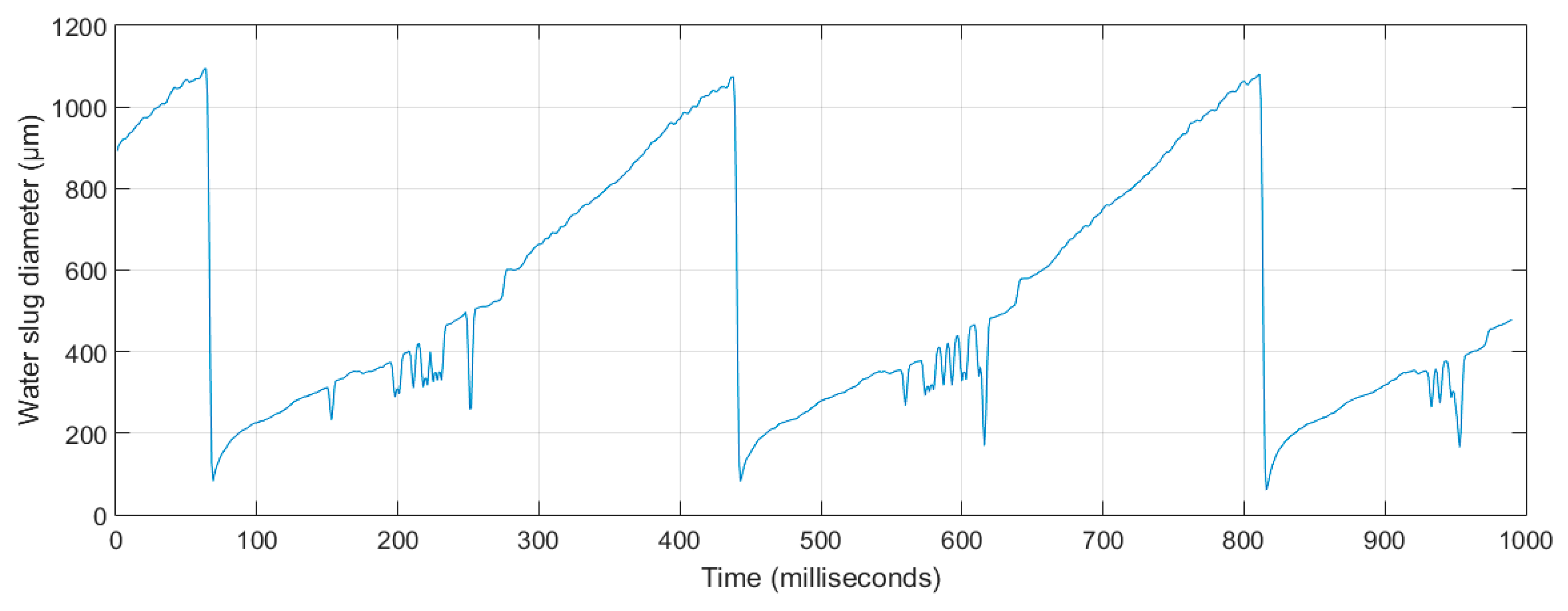
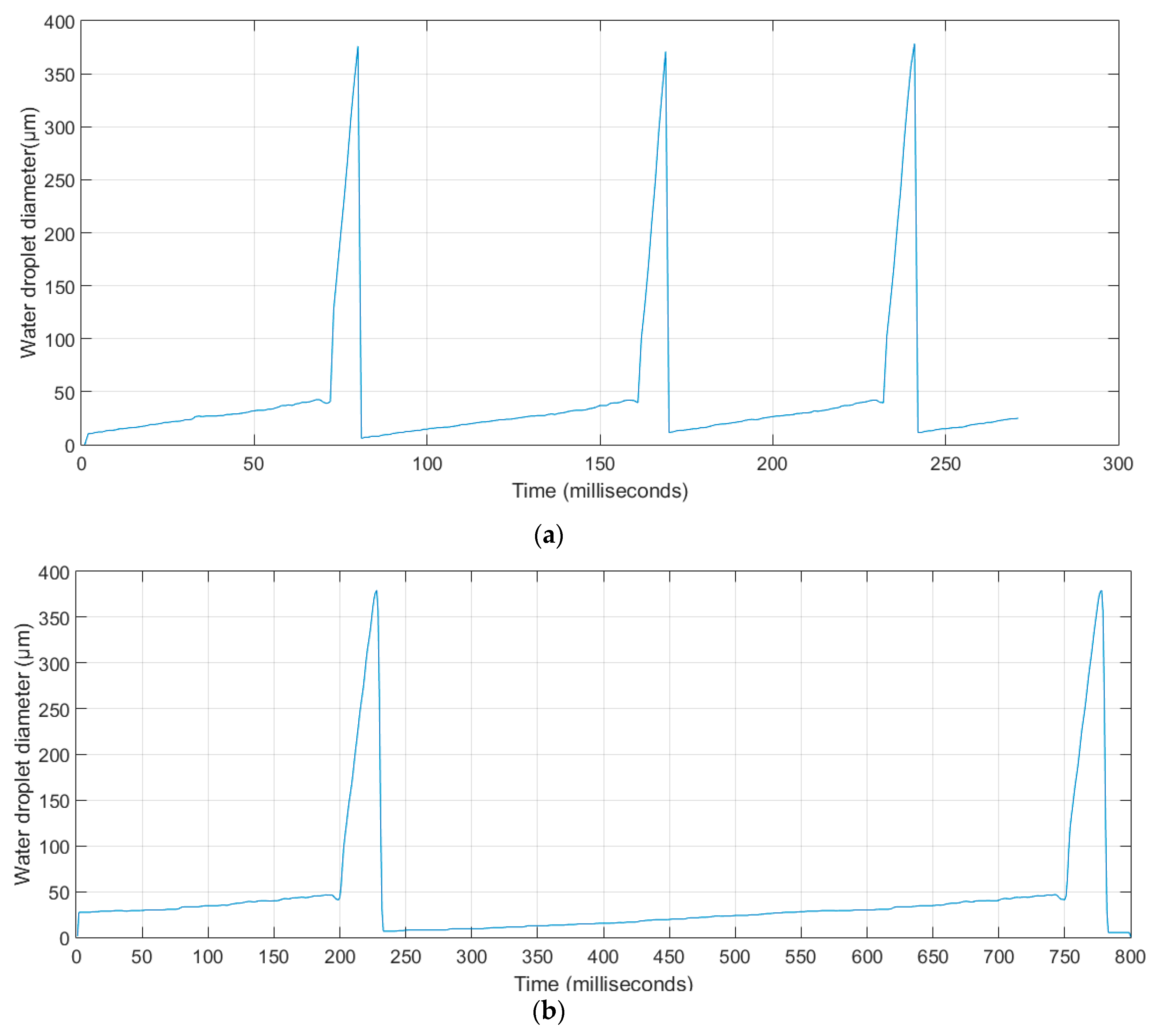
4.2.2. Geometric Characteristics
Base Diameter
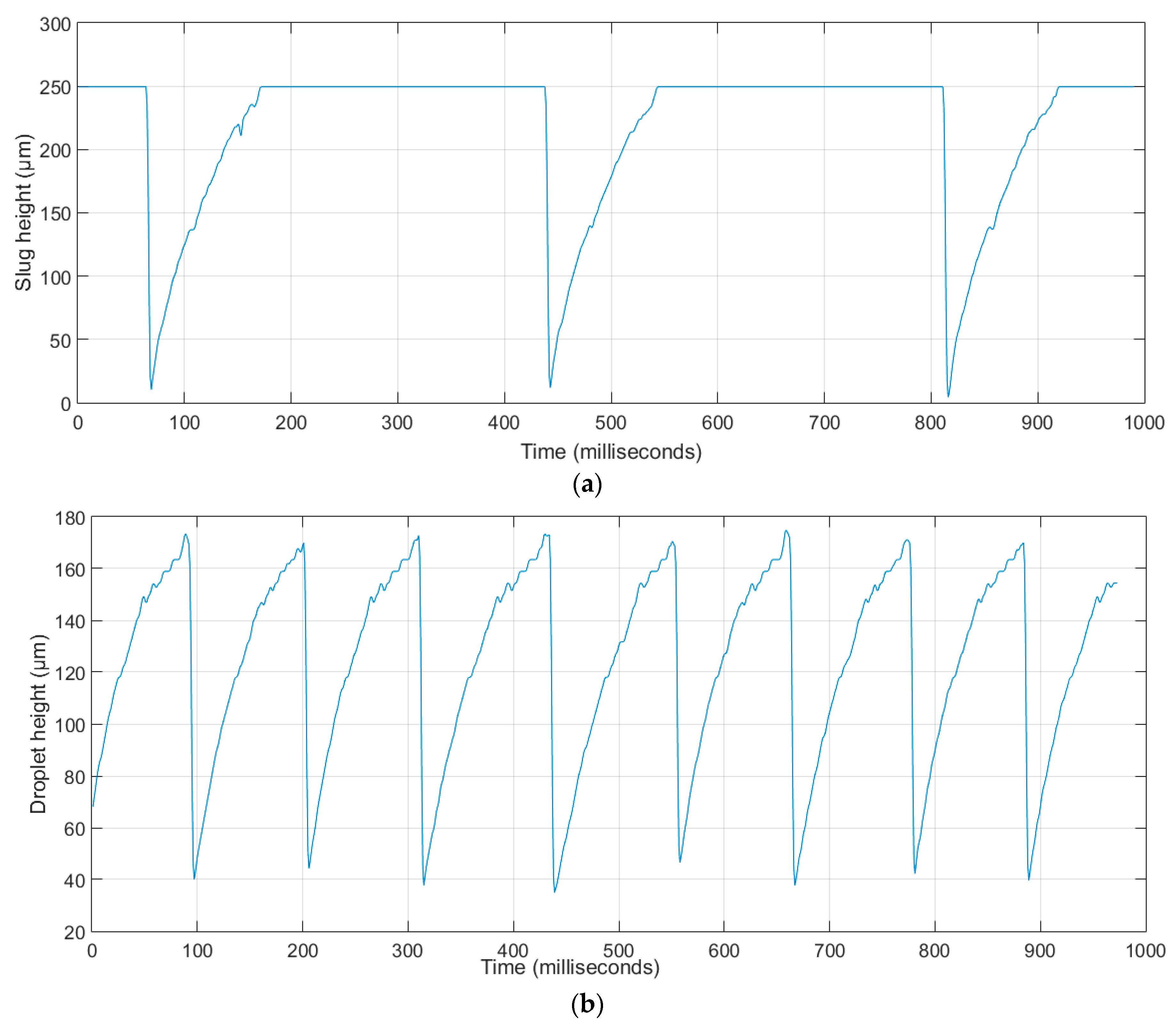
Height
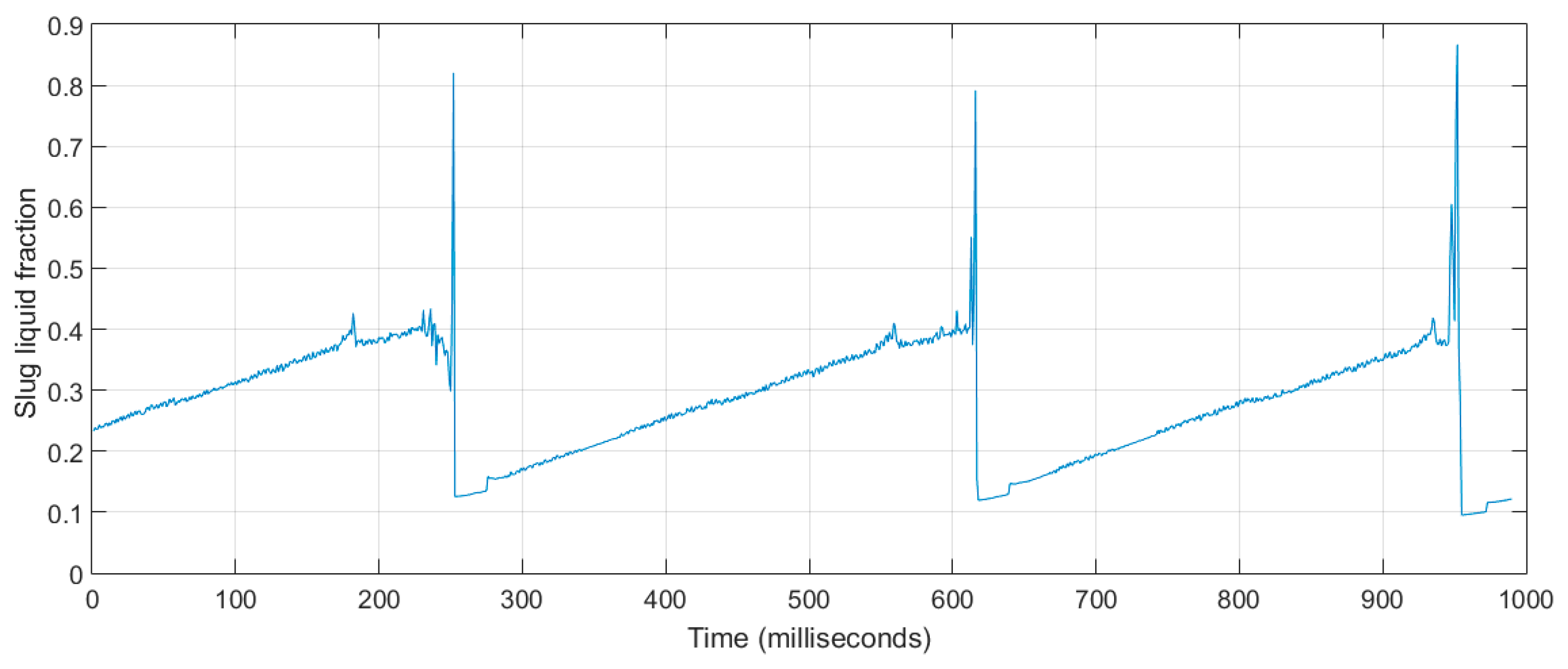
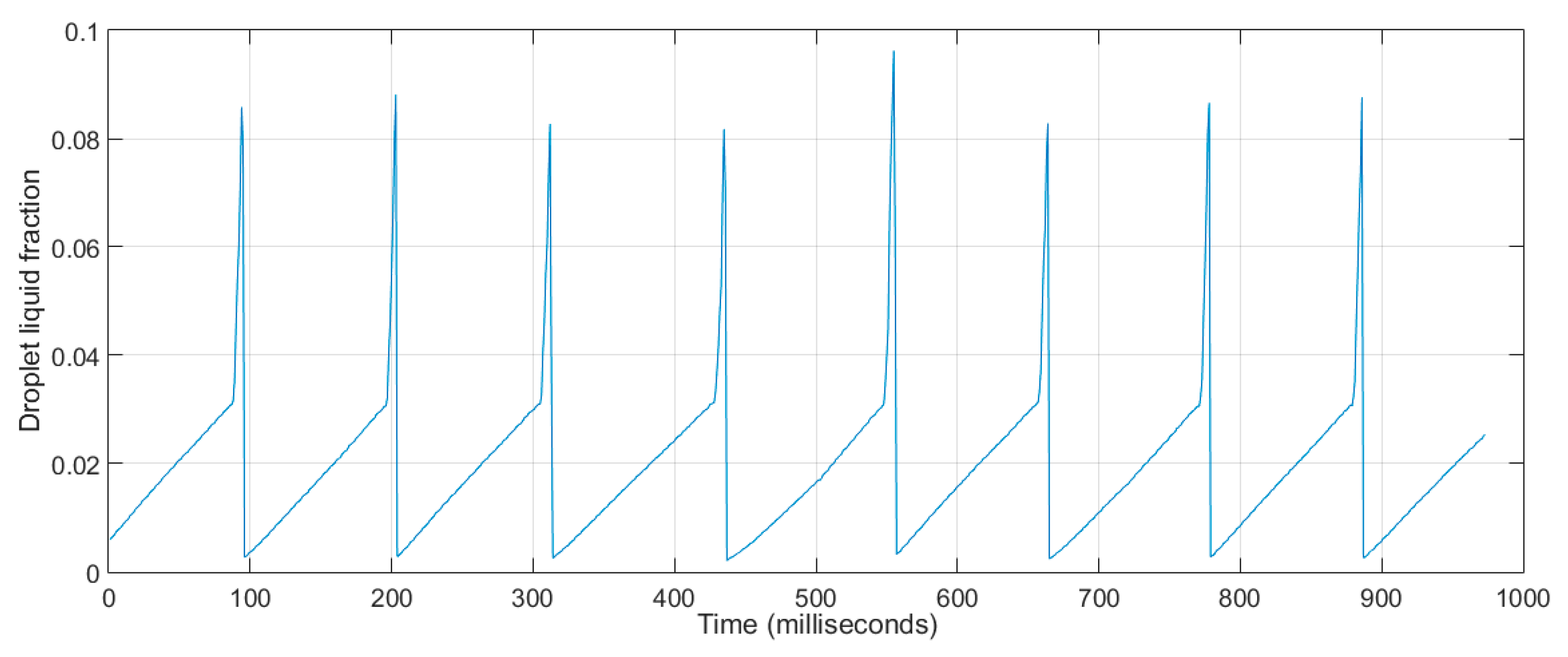
4.2.3. Liquid Fraction
4.2.4. Triple-Phase Point Contact Velocity
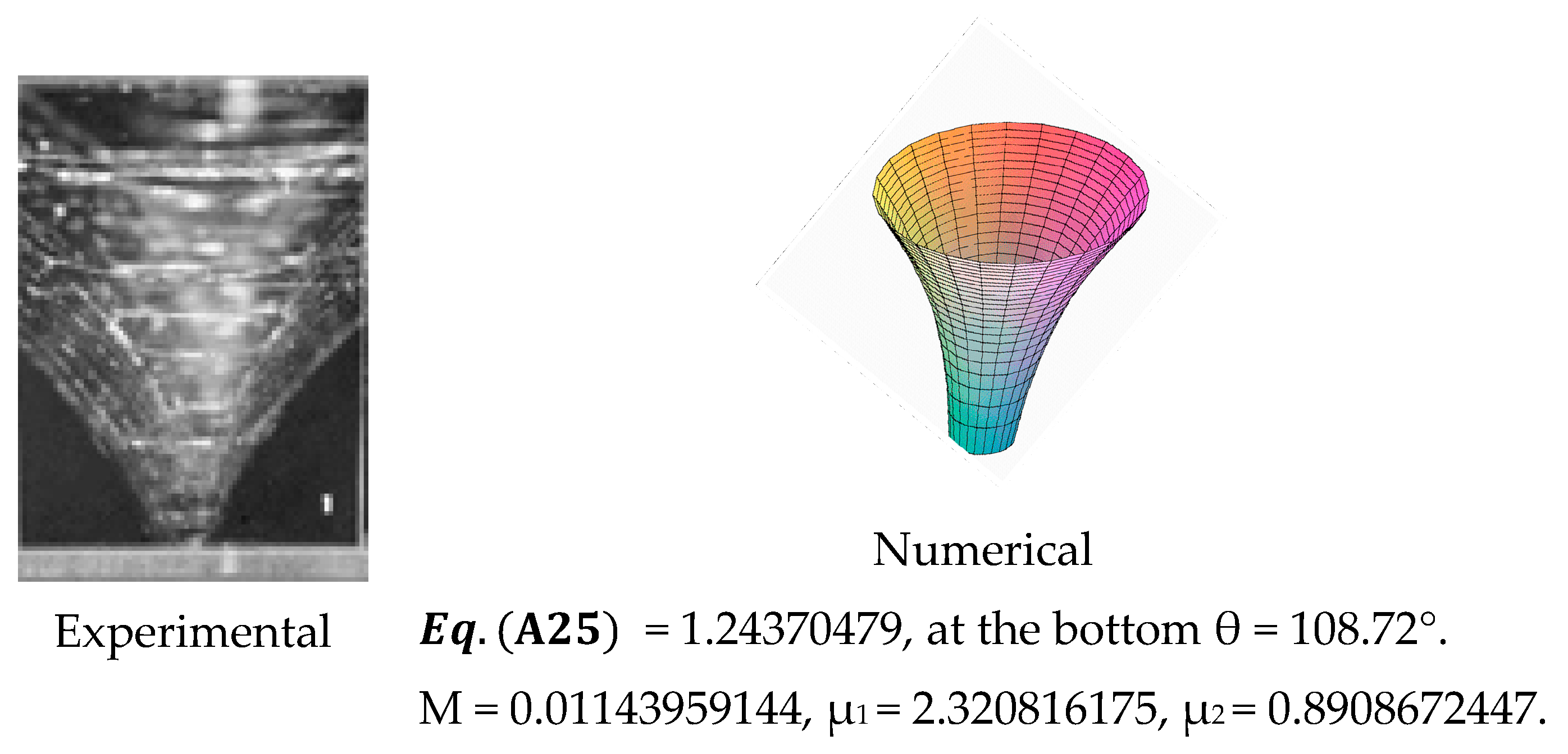
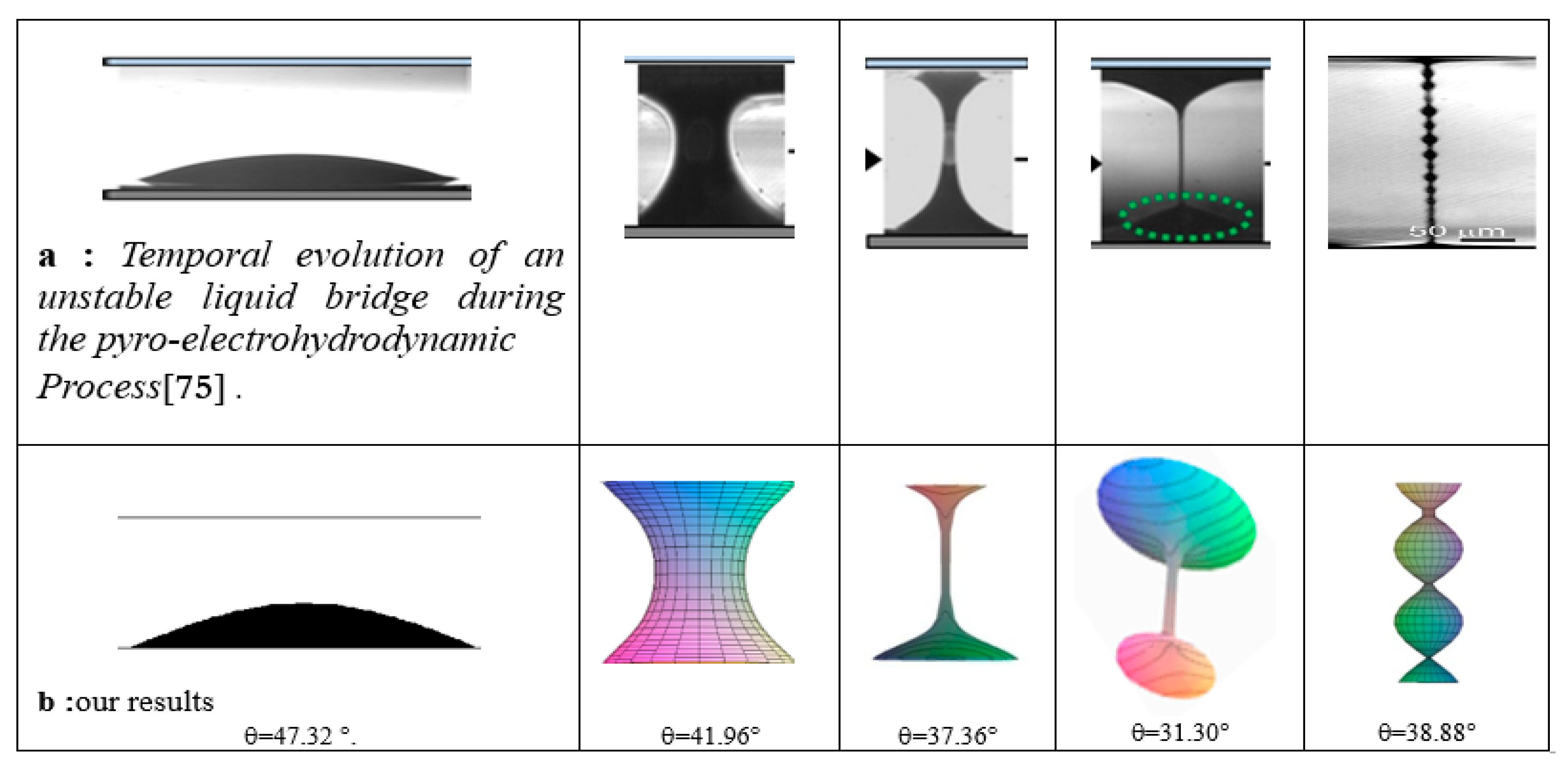
4.3. Liquid Bridge Regime: Comparison of Experiments and Model Predictions
5. Concluding Remarks
- Slug and water bridge (plug) flow are dominant at lower air-flow rates, whereas film flow is typically present at intermediate air flow and water droplet flow at higher air-flow rates.
- Water droplets are stable for extended periods (τ = 110 ms) without coalescence, and result in small liquid fractions (αwater = 0.085 to 0.12).
- Aside from slightly enhancing the spreading of water droplets and the film regime, gravity did not substantially affect the flow patterns in the range of Weber numbers investigated.
Author Contributions
Funding
Acknowledgments
Conflicts of Interest
Nomenclature
| Cross sectional area, | |
| Bond number | |
| Ca | Capillary number |
| g | Gravitational acceleration, m/s2 |
| H | Height, m |
| Mean curvature | |
| J | Superficial velocity, m/s |
| L | Length, m |
| P | Pressure, Pa |
| Pc | Capillary pressure, Pa |
| Q | Flow volume rate, for air in SCCM, for water in µl/min |
| S | Arc length along the liquid generator |
| T | Temperature, degree Celsius |
| t | Time, seconds |
| TPV | Triple point velocity, m/s |
| U | Change of variable, Equation (A6) |
| V | Volume, liter |
| Weber number | |
| Flow quality | |
| Abscissa where the liquid/air interface meets the GDL surface | |
| Greek symbols | |
| α | Volume fraction, % |
| β | First unknown constant, eq. |
| θ | Contact angle, degree |
| µ | Second unknown constant, eq. |
| Dynamic viscosity, Pa.s | |
| σ | Surface tension, N/m |
| τ | Period, seconds |
| φ | Explicit solution |
| ρ | Density, Kg/ |
| Subscripts | |
| 1, 2 | First and second roots |
| adv | Advancing |
| g | Gas (air) |
| h | Horizontal |
| l | Liquid (here, it’s water) |
| rec | Receding |
| T | Triple point (water/air/solid) |
| v | Vertical |
Appendix A

| Flow Pattern | [m/s] | [m/s] | Temp. [°C] | Pressure [Pa] | Interval Time [] | Droplet Height [] | Droplet Base Diameter [] | Liquid Fraction % | Time of Detachment [ms] | Volume at Detachment [nl] | ||
|---|---|---|---|---|---|---|---|---|---|---|---|---|
| For perpendicular flow | ||||||||||||
 Capillary Bridge concave | 40.0 | 0.00 | 22.88 | 114591 | 1000 | Bridge/plug 250 | Pore diameter | 65 | 65 | |||
 Capillary Bridge convex | 40.0 | 0.00 | 22.80 | 114798 | 1000 | 250 | θleft = 91.68 θright = 79.84 | θleft = 58.20 θright = 121.8 | ||||
 Droplet | 6.7 | 9.82 | 22.88 | 114591 | 1000 | 172 | 300 | 125° | 15° | 0.085 | 96.5 | 1.61 |
 Droplet flow | 13.3 | 9.57 | 23.01 | 114798 | 1000 | 170 | 305 | 125° | 20° | 0.085 | 102.0 | 3.40 |
 Droplet flow | 20.0 | 9.39 | 23.11 | 115075 | 1000 | 170 | 315 | 125° | 20° | 0.085 | 84.0 | 4.20 |
 Droplet flow | 27.0 | 9.47 | 23.27 | 114384 | 1000 | 170 | 322 | 125° | 20° | 0.085 | 98.0 | 6.50 |
 Slug flow | 40.0 | 1.60 | 24.03 | 114384 | 1000 | 250 | 1100 | 110° | 20° | 0.900 | 175.0 | 17.50 |
 Droplet flow | 40.0 | 10.00 | 23.88 | 114798 | 165 | 175 | 325 | 125° | 20° | 0.085 | 110.0 | 11.00 |
 Film flow | 40.0 | 4.00 | 24.20 | 115074 | 1000 | 179 | 1468 | 120° | 15° | 0.19 | 106.2 | 26.55 |
| For parallel flow | ||||||||||||
 Droplet flow | 40.0 | 10.00 | 23.88 | 114798 | 167 | 210 | 380 | 120° | 10° | 0.120 | 86.0 | 8.60 |
 Film flow | 40.0 | 4.00 | 24.03 | 115074 | 1000 | 187 | 1666 | 125° | 20° | 0.30 | 65.0 | 16.25 |
Appendix B. Derivation of Liquid Bridge Model
Appendix B.1. Governing Equations
Appendix B.2. Numerical Solution

| θ (°) | |λ| | 0.53 | U1 | U2 | μ | (Experimental) | Numerical | |
|---|---|---|---|---|---|---|---|---|
| 65° | 0.466 | Β = 0.909 | 0.6059230857 | 0.99885410 | 0.01143959144 | 405.0084 nl | 400.000 | 1.24 |
References
- Cheah, M.J.; Kevrekidis, I.G.; Benziger, J.B. Water slug to drop and film transitions in gas-flow channels. Langmuir 2013, 29, 15122–15136. [Google Scholar] [CrossRef] [PubMed]
- Chinnov, E.A.; Ron’shin, F.V.; Kabov, O.A. Regimes of two-phase flow in micro- and mini-channels. Thermophys. Aeromech. 2015, 22, 265–284. [Google Scholar] [CrossRef]
- Kakaç, S.; Yenner, Y.; Pramuanjaroenkij, A. Convective Heat Transfer, 3rd ed.; CRC Press, Taylor and Francis: Boca Raton, FL, USA, 2014; ISBN 9781466583443. [Google Scholar]
- Qu, J.; Wu, H.; Cheng, P. Start-up, heat transfer and flow characteristics of silicon-based micro pulsating heat pipes. Int. J. Heat Mass Transf. 2012, 55, 6109–6120. [Google Scholar] [CrossRef]
- Wu, H.Y.; Cheng, P. An experimental study of convective heat transfer in silicon microchannels with different surface conditions. Int. J. Heat Mass Transf. 2003, 46, 2547–2556. [Google Scholar] [CrossRef]
- Ong, C.L.; Thome, J.R. Macro-to-microchannel transition in two-phase flow, Part 1: Two-phase flow patterns and film thickness measurements. Exp. Therm. Fluid Sci. 2011, 35, 37–47. [Google Scholar] [CrossRef]
- Wang, P.; McCluskey, P.; Bar-Cohen, A. Two-Phase Liquid Cooling for Thermal Management of IGBT Power Electronic Module. J. Electron. Packag. 2013, 135, 021001. [Google Scholar] [CrossRef]
- Basauri, A.; Gomez-Pastora, J.; Fallanza, M.; Bringa, E.; Ortiz, I. Predictive model for the design of reactive micro-separations. Sep. Purif. Technol. 2019, 209, 900–907. [Google Scholar] [CrossRef]
- Zheng, Y. Liquid Plug Dynamics in Pulmonary Airways. Ph.D. Thesis, Biomedical Engineering, University of Michigan, Ann Arbor, MI, USA, 2008. [Google Scholar]
- Yang, H.; Zhao, T.S.; Ye, Q. In-situ visualization study of CO2 gas bubble behavior in DMFC anode flow fields. J. Power Sources 2005, 139, 79–90. [Google Scholar] [CrossRef]
- Djilali, N. Computational modelling of PEM fuel cells: Challenges and opportunities. Energy 2007, 32, 269–280. [Google Scholar] [CrossRef]
- Wu, T.C.; Djilali, N. Experimental investigation of water droplet emergence in a model polymer electrolyte membrane fuel cell microchannel. J. Power Sources 2012, 208, 248–256. [Google Scholar] [CrossRef][Green Version]
- Kandlikar, S.; Lu, Z.; Trabold, T.; Owejan, J.; Gagliardo, J.; Allen, J.; Shahbazian-Yassar, R. Visualization of Fuel Cell Water Transport and Performance Characterization under Freezing Conditions; Final Technical Report; U.S. Department of Energy: Washington, DC, USA, 2010.
- Zhan, Z.; Zhao, H.; Sui, P.C.; Jiang, P.; Pan, M.; Djilali, N. Numerical analysis of ice-induced stresses in the membrane electrode assembly of a PEM fuel cell under sub-freezing operating conditions. Int. J. Hydrogen Energy 2018, 43, 4563–4582. [Google Scholar] [CrossRef]
- Shen, J.; Liu, Z.; Liu, F.; Liu, W. Numerical Simulation of Water Transport in a Proton Exchange Membrane Fuel Cell Flow Channel. Energies 2018, 11, 1770. [Google Scholar] [CrossRef]
- Chevalier, S.; Ge, N.; Lee, J.; George, M.G.; Liu, H.; Shrestha, P.; Muirhead, D.; Lavielle, N.; Hatton, B.D.; Bazylak, A. Novel electrospun gas diffusion layers for polymer electrolyte membrane fuel cells: Part II. In operando synchrotron imaging for microscale liquid water transport characterization. J. Power Sources 2017, 352, 281–290. [Google Scholar] [CrossRef]
- Hasanpour, S.; Ahadi, M.; Bahrami, M.; Djilali, N.; Akbari, M. Woven gas diffusion layers for polymer electrolyte membrane fuel cells: Liquid water transport and conductivity trade-offs. J. Power Sources 2018, 403, 192–198. [Google Scholar] [CrossRef]
- Steinbrenner, J.E.; Lee, E.S.; Wang, F.M.; Fang, C.; Hidrovo, C.H.; Goodson, K.E. Flow regime evolution in long, serpentine micro channels with a porous carbon paper wall. In Proceedings of the ASME 2008 International Mechanical Engineering Congress and Exposition, Boston, MA, USA, 31 October–6 November 2008; pp. 773–781. [Google Scholar]
- Steinbrenner, J.E.; Lee, E.S.; Hidrovo, C.H.; Eaton, J.K.; Goodson, K.E. Impact of channel geometry on two-phase flow in fuel cell micro channels. J. Power Sources 2011, 196, 5012–5020. [Google Scholar] [CrossRef]
- Cho, S.C.; Wang, Y.; Chen, K.S. Droplet dynamics in a polymer electrolyte fuel cell gas flow channel: Forces, deformation, and detachment, I: Theoretical and numerical analyses. J. Power Sources 2012, 206, 119–128. [Google Scholar] [CrossRef]
- Coleman, J.W.; Garimella, S. Characterization of two-phase flow patterns in small-diameter round and rectangular tubes. Int. J. Heat Mass Transf. 1999, 42, 2869–2881. [Google Scholar] [CrossRef]
- Serizawa, A.; Feng, Z.; Kawara, Z. Two-phase flow in micro-channels. Exp. Therm. Fluid Sci. 2012, 26, 703–714. [Google Scholar] [CrossRef]
- Jarauta, A.; Ryzhakov, P. Challenges in Computational Modeling of Two-Phase Transport in Polymer Electrolyte Fuel Cells Flow Channels: A Review. Arch. Comput. Methods Eng. 2018, 25, 1027–1057. [Google Scholar] [CrossRef]
- Bazylak, A. Liquid water visualization in PEM fuel cells: A review. Int. J. Hydrogen Energy 2009, 34, 3845–3857. [Google Scholar] [CrossRef]
- George, R.B.; Light, R.W.; Matthay, M.A. Chest Medicine: Essentials of Pulmonary and Critical Care Medicine, 2nd ed.; Williams & Wilkins: Baltimore, MD, USA, 1990; 512p. [Google Scholar]
- Gorb, S.N. The design of the fly adhesive pad: Distal tenent setae are adapted to the delivery of an adhesive secretion. Proc. R. Soc. Lond. B Biol. Sci. 1998, 265, 747–752. [Google Scholar] [CrossRef]
- Melrose, J.C. Model calculations for capillary condensation. AIChE J. 1996, 12, 986–994. [Google Scholar] [CrossRef]
- Zasadzinski, J.N.; Sweeney, J.B.; Davis, H.T.; Scriven, L.E. Finite-element calculation of fluid menisci and thin films in model porous media. J. Colloid Interface Sci. 1987, 119, 108–116. [Google Scholar] [CrossRef]
- Witkowski, L.M.; Walker, J.S. Solutocapillary instabilities in liquid bridges. Phys. Fluids 2002, 14, 2647–2656. [Google Scholar] [CrossRef]
- Fisher, R.A. On the capillary forces in an ideal soil. J. Agric. Sci. 1926, 16, 492–505. [Google Scholar] [CrossRef]
- Israelachvili, J.N. Intermolecular and Surface Forces, 2nd ed.; Academic Press: London, UK, 1992. [Google Scholar]
- Kralchevsky, P.A.; Nagayama, K. Capillary Bridges and Capillary-Bridge Forces. Stud. Interface Sci. 2001, 10, 469–502. [Google Scholar]
- Klaas, M.; Koch, E.; Schröder, W. Fundamental medical and engineering investigations on protective artificial respiration. In Notes on Numerical Fluid Mechanical and Multidisciplinary Design; Springer: Berlin/Heidelberg, Germany, 2011; Volume 116, pp. 78–80. [Google Scholar]
- Gomez, M.; Parra, I.E.; Perales, J.M. Mechanical imperfections effect on the minimum volume stability limit of liquid bridges. Phys. Fluids 2002, 14, 2029–2042. [Google Scholar] [CrossRef]
- Shevtsova, V.; Gaponenko, Y.A.; Nepomnyashchy, A. Thermocapillary tow regimes and instability caused by a gas stream along the interface. J. Fluid Mech. 2013, 714, 644–670. [Google Scholar] [CrossRef]
- Qian, B.; Kenneth, S.B. The motion, stability and breakup of stretching liquid bridge with a receding contact angle. J. Fluid Mech. 2011, 666, 554–572. [Google Scholar] [CrossRef]
- Kralchevsky, P.A.; Denskov, N.D. Capillary forces and structuring in layers of colloid particles. J. Curr. Opin. Colloid Interface Sci. 2001, 6, 383–401. [Google Scholar] [CrossRef]
- Yang, L.; Tuabc, Y.; Fang, H. Modeling the rupture of a capillary liquid bridge between a sphere and plane. Soft Matter R. Soc. Chem. 2010, 24, 6178–6182. [Google Scholar] [CrossRef]
- Hoang, D.A.; van Steijn, V.; Portela, L.M.; Kreutzer, M.T.; Kleijn, C.R. Benchmark numerical simulations of segmented two-phase flows in microchannels using the Volume of Fluid method. Comput. Fluids 2013, 86, 28–36. [Google Scholar] [CrossRef]
- Li, S.Z.; Chen, R.; Wang, H.; Liao, Q.; Zhu, X.; Wang, Z.B.; He, X.F. Numerical investigation of the moving liquid column coalescing with a droplet in triangular microchannels using CLSVOF method. Sci. Bull. 2015, 60, 1911–1926. [Google Scholar] [CrossRef]
- Theodorakakos, A.; Ous, T.; Gavaises, A.; Nouri, J.M.; Nikolopoulos, N.; Yanagihara, H. Dynamics of water droplets detached from porous surfaces of relevance to PEM fuel cells. J. Colloid Interface Sci. 2006, 300, 673–687. [Google Scholar] [CrossRef]
- Zhu, X.; Sui, P.C.; Djilali, N. Numerical simulation of emergence of a water droplet from a pore into a microchannel gas stream. Microfluid. Nanofluid. 2008, 4, 543–555. [Google Scholar] [CrossRef]
- Zhu, X.; Sui, P.C.; Djilali, N. Three-dimensional numerical simulations of water droplet dynamics in a PEMFC gas channel. J. Power Sources 2008, 181, 101–115. [Google Scholar] [CrossRef]
- Zhu, X.; Liao, Q.; Sui, P.C.; Djilali, N. Numerical investigation of water droplet dynamics in a low-temperature fuel cell microchannel: Effect of channel geometry. J. Power Sources 2010, 195, 801–812. [Google Scholar] [CrossRef]
- Yang, K.; Guo, Z.L. Multiple-relaxation-time lattice Boltzmann model for binary mixtures of nonideal fluids based on the Enskog kinetic theory. Sci. Bull. 2015, 60, 634–647. [Google Scholar] [CrossRef]
- Zhu, X.; Sui, P.C.; Djilali, N. Dynamic behaviour of liquid water emerging from a GDL pore into a PEMFC gas flow channel. J. Power Sources 2007, 172, 287–295. [Google Scholar] [CrossRef]
- Qin, Y.; Wang, X.; Chen, R.; Shangguan, X. Water Transport and Removal in PEMFC Gas Flow Channel with Various Water Droplet Locations and Channel Surface Wettability. Energies 2018, 11, 880. [Google Scholar] [CrossRef]
- Tobias, M.; Nils, P.; Muller, C.; Zengerle, R.; Koltay, P. Passive water removal in fuel cells by capillary droplet actuation. Sens. Actuators A Phys. 2008, 143, 49–57. [Google Scholar]
- Niu, Z.; Wang, R.; Jiao, K.; Du, Q.; Yin, Y. Direct numerical simulation of low Reynolds number turbulent air-water transport in fuel cell flow channel. Sci. Bull. 2017, 62, 31–39. [Google Scholar] [CrossRef]
- Minor, G.; Djilali, N.; Sinton, D.; Oshkai, P. Flow within a water droplet subjected to an air stream in a hydrophobic microchannel. Fluid Dyn. Res. 2009, 41, 045506. [Google Scholar] [CrossRef]
- Lee, S.J.; Lim, S.K.; Park, G.G.; Kim, C.S. X-ray imaging of water distribution in a polymer electrolyte fuel cell. J. Power Sources 2008, 185, 867–870. [Google Scholar] [CrossRef]
- Minard, K.R.; Viswanathan, V.V.; Majors, P.D.; Wang, L.Q.; Rieke, P.C. Magnetic resonance imaging (MRI) of PEM dehydration and gas manifold flooding during continuous fuel cell operation. J. Power Sources 2006, 161, 856–863. [Google Scholar] [CrossRef]
- Feindel, K.; LaRocque, L.A.; Starke, D.; Bergens, S.; Wasylishen, R. In-situ observations of water production and distribution in an operating H2/O2 PEM fuel cell assembly using 1H NMR microscopy. J. Am. Chem. Soc. 2004, 126, 11436–11437. [Google Scholar] [CrossRef]
- Lu, Z.; Daino, M.M.; Rath, C.; Kandlikar, S.G. Water management studies in PEM fuel cells, Part III: Dynamic breakthrough and intermittent drainage characteristics from GDLs with and without MPLs. Int. J. Hydrogen Energy 2010, 35, 4222–4233. [Google Scholar] [CrossRef]
- Tuber, K.; Pocza, D.; Hebling, C. Visualization of water buildup in the cathode of a transparent PEM fuel cell. J. Power Sources 2003, 124, 403–414. [Google Scholar] [CrossRef]
- Poisson, S.D. Nouvelle Théorie de L’action Capillaire; Bachelier Père et Fils: Quai des Augustins, Paris, France, 1830. [Google Scholar]
- Plateau, J. Experimental and Theoretical Researches on the Figures of Equilibrium of a Liquid Mass Withdrawn from the Action of Gravity; Annual Report of the Smithsonian Institution: Washington, DC, USA, 1863; pp. 207–285. [Google Scholar]
- Lord Rayleigh. On the instability of jets. Proc. Lond. Math. Soc. 1879, 10, 4–13. [Google Scholar]
- Slobozhanin, L.A.; Perales, J.M. Stability of liquid bridges between equal disks in an axial gravity field. Phys. Fluids A 1993, 5, 1305–1314. [Google Scholar] [CrossRef]
- Da Riva, I.; Martinez, I. Floating Zone Stability; Exp 1-ES-331, In ESA SP-14; European Space Agency: Paris, France, 1979; pp. 67–73. [Google Scholar]
- Gillette, R.D.; Dyson, D.C. Stability of fluid interfaces of revolution between equal solid circular plates. J. Chem. Eng. 1971, 2, 44–54. [Google Scholar] [CrossRef]
- Meseguer, J.; Espino, J.; Perales, J.M.; Laveron-Simavilla, A. On the breaking of long, axisymmetric liquid bridges between unequal supporting disks at minimum volume stability limit. Eur. J. Mech. B Fluids 2003, 22, 355–368. [Google Scholar] [CrossRef]
- Orr, F.M.; Scriven, L.E.; Rivas, A.P. Pendular rings between solids: Meniscus properties and capillary force. J. Fluid Mech. 1975, 67, 723–742. [Google Scholar] [CrossRef]
- Wiklund, H. Lattice Boltzmann Simulations of Two-Phase Flow in Fibre Network Systems. Ph.D. Thesis, Mid-Sweden University, Sundsvall, Sweden, 2012. [Google Scholar]
- Anderson, R.; Zhang, L.; Ding, Y.; Blanco, M.; Bi, X.; Wilkinson, D.P. A critical review of two-phase flow in gas channels of PEM fuel cells. J. Power Sources 2010, 195, 4531–4553. [Google Scholar] [CrossRef]
- Wörner, M. Numerical modeling of multiphase flows in microfluidics and micro process engineering: A review of methods and applications. Microfluid. Nanofluid. 2012, 12, 841–886. [Google Scholar] [CrossRef]
- Canny, J. A computational approach to edge detection. IEEE Trans. Pattern Anal. Mach. Intell. 1986, 8, 679–698. [Google Scholar] [CrossRef]
- Rynhart, P.; McKibbin, R.; McLachlan, R.; Jones, J.R. Mathematical modelling of granulation: Static and dynamic liquid bridges. Res. Lett. Inf. Math. Sci. 2002, 3, 199–212. [Google Scholar]
- Kenmotsu, K. Surfaces of revolution with prescribed mean curvature Tohoku. Math. J. 1980, 32, 147–153. [Google Scholar]
- Kenmotsu, K. Surfaces of revolution with periodic mean curvature. Osaka J. Math. 2003, 40, 687–696. [Google Scholar]
- Gu, H.; Duits, M.H.G.; Mugele, F. Droplet formation and merging in two-phase flow microfluidics. Int. J. Mol. Sci. 2011, 12, 2572–2597. [Google Scholar] [CrossRef]
- Herrada, M.A.; López-Herrera, J.M.; Vega, E.J.; Montanero, J.M. Numerical simulation of a liquid bridge in a coaxial gas flow. Phys. Fluids 2011, 23, 012101. [Google Scholar] [CrossRef]
- Vega, E.J.; Montanero, J.M.; Herrada, M.A.; Ferrera, C. Dynamics of an axisymmetric liquid bridge close to the minimum-volume stability limit. Phys. Rev. E 2014, 90, 013015. [Google Scholar] [CrossRef]
- Fernando, R.H.; Xing, L.-L.; Glass, J.E. Erratum to Rheology parameters controlling spray atomization and roll misting behavior of waterborne coatings. Prog. Org. Coat. 2001, 42, 284–288. [Google Scholar] [CrossRef]
- Grilli, S.; Coppola, S.; Vespini, V.; Merola, F.; Finizio, A.; Ferraro, P. 3D lithography by rapid curing of the liquid instabilities at nanoscale. Proc. Natl. Acad. Sci. USA 2011, 108, 15106–15111. [Google Scholar] [CrossRef] [PubMed]
- Broesch, D.; Frechette, J. From concave to convex: Capillary bridges in slit pore geometry. Langmuir 2012, 28, 15548–15554. [Google Scholar] [CrossRef]


| Channel length | L = 1000 m |
| Chanel height | H = 250 m |
| Channel width | W = 250 m |
| Pore diameter | d = 50 m |
| Gas volume rate | Qair ≈ 0–15 SCCM |
| Liquid volume rate | Qw = 6 L/min |
| Inlet temperature | T = 22 °C |
| Inlet pressure | P = 1.11 bar |
| Bond number | B = 3.36 × 10⁻⁴ |
| Capillary number | Ca = 5.5 × 10⁻⁴ |
| Capillary pressure | Pc = 288 Nm−2 |
| Gas Superficial Velocity | Volume Fraction α | Flow Quality | Temperature T (°C) | Pressure P (kPa) | (μs) |
|---|---|---|---|---|---|
| Dry air conditions | Dry air conditions | Dry air conditions | 22.88 | 114.59 | 1000 |
| 1.6 | 0.976 | 0.051 | 24.03 | 114.38 | 1000 |
| 4 | 0.990 | 0.120 | 24.03 | 115.07 | 1000 |
| 10 | 0.996 | 0.256 | 23.88 | 114.79 | 167 |
| Numerical Results | Experimental Recording | Liquid Volume, Contact Angle |
|---|---|---|
 |  | a: convex shape Volume = 890nl, θleft = 91.68° θright = 60.78° |
 |  | b: concave shape Volume = 201 nl, θleft = θright = 65°. |
 |  | c: t = 4050 ms Volume = 405 nl, θleft = 91.68°, θright = 79.84° |
 |  | d: t = 4286 ms Volume = 429 nl θleft = 58.20°.θright = 121.8° |
 |  | e: sessile droplet Volume ≈ 334 nl. θleft = θright = 57.96°. |
 |  | f: liquid bridge with sessile droplet (last image in experiment) t = 4624 ms Volume = 463 nl. |
| Liquid bridge with sessile droplet obtained separately |
© 2019 by the authors. Licensee MDPI, Basel, Switzerland. This article is an open access article distributed under the terms and conditions of the Creative Commons Attribution (CC BY) license (http://creativecommons.org/licenses/by/4.0/).
Share and Cite
Ibrahim-Rassoul, N.; Si-Ahmed, E.-K.; Serir, A.; Kessi, A.; Legrand, J.; Djilali, N. Investigation of Two-Phase Flow in a Hydrophobic Fuel-Cell Micro-Channel. Energies 2019, 12, 2061. https://doi.org/10.3390/en12112061
Ibrahim-Rassoul N, Si-Ahmed E-K, Serir A, Kessi A, Legrand J, Djilali N. Investigation of Two-Phase Flow in a Hydrophobic Fuel-Cell Micro-Channel. Energies. 2019; 12(11):2061. https://doi.org/10.3390/en12112061
Chicago/Turabian StyleIbrahim-Rassoul, N., E.-K. Si-Ahmed, A. Serir, A. Kessi, J. Legrand, and N. Djilali. 2019. "Investigation of Two-Phase Flow in a Hydrophobic Fuel-Cell Micro-Channel" Energies 12, no. 11: 2061. https://doi.org/10.3390/en12112061
APA StyleIbrahim-Rassoul, N., Si-Ahmed, E.-K., Serir, A., Kessi, A., Legrand, J., & Djilali, N. (2019). Investigation of Two-Phase Flow in a Hydrophobic Fuel-Cell Micro-Channel. Energies, 12(11), 2061. https://doi.org/10.3390/en12112061