State Rules Mining and Probabilistic Fault Analysis for 5 MW Offshore Wind Turbines

Abstract

Research on fault identification for wind turbines (WTs) is a widespread concern. However, the identification accuracy in existing research is vulnerable to uncertainty in the operation data, and the identification results lack interpretability. In this paper, a data-driven method for fault identification of offshore WTs is presented. The main idea is to improve fault identification accuracy and facilitate the probabilistic sorting of possible faults with critical variables so as to provide abundant and reliable reference information for maintenance personnel. In the stage of state rule mining, representative initial rules are generated via the combination of a clustering algorithm and heuristic learning. Then, a multi-population quantum evolutionary algorithm is utilized to optimize the rule base. In the stage of fault identification, abnormal states are identified via a fuzzy rule-based classification system, and probabilistic fault sorting with critical variables is realized according to the fuzzy reasoning of state rules. Ten common sensor and actuator faults in 5 MW offshore WTs are taken to verify the feasibility and superiority of the proposed scheme. Experimental results demonstrate that the proposed method has higher identification accuracy than other identification methods and thus prove the feasibility of the proposed probabilistic fault analysis scheme.

1. Introduction

In recent years, research into renewable energy has attracted considerable attention owing to energy shortages and increasingly serious environmental problems [1]. Wind power generation, as one of the most hopeful green renewable energy sources, is developing rapidly throughout the world. The ratio of offshore wind turbines (WTs) has increased gradually to benefit from strong and substantially uniform wind regimes [2]. For offshore WTs, approximately 15–35% of the total expense is used for operation and maintenance [3]. Therefore, the timely detection and accurate location of common faults are crucial to enhance the efficiency of offshore WTs.

Existing research divides the methods for fault detection and identification (FDI) for WTs into model-based and data-based methods [4]. Model-based methods include state estimation, state filter, and redundancy analysis [5,6]. Mojallal et al. [7] proposed a multi-physics graphical fault detection and classification scheme for WTs. The model of the WT is obtained through hybrid bond–graph theory that captures the causal, temporal, and structural properties of the system. Laouti et al. [8] proposed a combination scheme of observer and support vector machines (SVMs) for fault detection of WTs. This scheme utilizes structural risk minimization to enhance generalization with a small training data set, and it allows for process nonlinearity by using flexible kernels. Cho et al. [9] proposed a model-based method for fault detection of blade pitch systems, designed a Kalman filter to estimate blade pitch angle. As the building of system models is dependent on expert knowledge [10], data acquisition and data mining technologies have made considerable progress [11]. Consequently, data-based methods have received increasing attention in the area of fault detection and location of WTs [12].

In data-based research, substantial improvements have been proposed to improve the accuracy of fault identification. Chen et al. [13] proposed a fault prediction method for WTs using an adaptive neuro-fuzzy inference system with a priori knowledge. This method provides a fault instruction and allows the operator to determine the repair plan before the failure worsens. Hu et al. [14] proposed a fault diagnosis method that combines SVM and domain knowledge to improve the identification accuracy for faults in WTs. However, the aforementioned methods depend excessively on expert knowledge, and their identification results are simplistic. Wang et al. [15] proposed an FDI scheme based on a variable selection method using principal component analysis; in this scheme, the result of fault identification is determined by the signal contribution, but the method can only identify an abnormal signal rather than a fault type. Ruiz et al. [16] proposed a fault classification method for WTs that transforms the domain signals of WTs into two-dimensional matrices. Certain similar faults are merged for identification in the experiment, and the separation of similar faults is unwarrantable. Pashazadeh et al. [17] obtained the fault data of WTs from the Fatigue, Aerodynamics, Structures, and Turbulence (FAST) simulator and Simulink (in a MATLAB environment) and developed an FDI scheme on the basis of classifier fusion, in which four classifiers are implemented in parallel. However, this method can only provide a single identification result, and the method’s algorithm implementation and parameter settings are complicated. For the data-based methods mentioned above, their identification accuracies remain unsatisfactory, and the results always ignore the importance of interpretability to the maintainer. These problems may cause a delay in maintenance time and increase maintenance cost.

The present study investigates a probabilistic fault identification scheme on the basis of the fuzzy rule-based classification system (FRBCS) to improve the accuracy of fault identification and enhance the interpretability of identification results for offshore WTs. In the mining of state rules, initial state rules are generated via the combination of a clustering algorithm and heuristic learning. Moreover, a multi-population quantum evolutionary algorithm (MPQEA) with a hybrid evolutionary strategy is utilized to optimize the rule set. In the stage of fault identification, the fuzzy reasoning method of FRBCS is adopted to identify the operating states of WTs. A probability analysis scheme for the abnormal state is also proposed to realize the probabilistic sorting of possible faults with crucial state features.

This paper is organized as follows: Section 2 presents a rule mining scheme of operating state for offshore wind turbine. The fault descriptions and the complete scheme of fault identification and probability analysis are described in Section 3. Numerical experiments and fault identification experiments are performed in Section 4. Finally, Section 5 summarizes the conclusions.

2. Rule Mining of Operating States for Offshore WTs using MPQEA

In this section, a state rule mining method is introduced for an offshore WT. The fuzzy reasoning process of FRBCS is reviewed in Section 2.1, the fuzzy classification rule mining method based on multi-population quantum evolutionary optimization (MPQEA-FRBCS) is introduced in Section 2.2, including the generation of the initial population, the multi-population quantum coding method, and the optimization of the fuzzy rules set using the hybrid updating strategy.

2.1. Fuzzy Rule-Based Classification Systems

FRBCSs [18] are widely used because of their ability to provide interpretable language models for users, and the possibility of information fusion with expert knowledge, mathematical models, and empiric measures [19]. FRBCSs are mainly composed of a knowledge base and reasoning strategy [20].

• Knowledge base: Including the fuzzy rule base and data base.
• Reasoning strategy: The classification mechanism of samples using the fuzzy rules in the knowledge base.

For an n-dimensional M-class classification problem with m training samples, and each variable is described by given linguistic labels. The form of fuzzy rules for the above classification problem is as follows [20]:

$$Rule R_q:if x_1 is A_{q1} and ,\dots , and x_n is A_{qn}, then Class is C_q with R{W}_q,q=1,2,\dots ,N_r$$

(1)

where x = (x₁, …, x_n) is a training sample, A_qi is the i-th antecedent, C_q is the class label, RW_q is the rule weight of the q-th fuzzy rule, and N_r is the number of rules. The classification process of the new sample x_p = (x_p1,…,x_pn) in FRBCSs is described as follows [19]:

2.1.1. Match Degree

For a sample x_p, its match degree to each rule is the product of membership degrees in all antecedents [19]:

$${\mu }_{{\mathbf{A}}_q}({\mathbf{x}}_p)={\mu }_{A_{q1}}(x_{p1})\cdot {\mu }_{A_{q2}}(x_{p2})\cdot \dots \cdot {\mu }_{A_{qn}}(x_{pn})$$

(2)

where, μ_Aqi(·) is the membership function of the i-th antecedent in the q-th rule.

2.1.2. Rule Weight

For the rule weight (RW), the Penalized Certainty Factor (PCF) for multi-class problems in [21] is adopted:

$$R{W}_q=\frac{{\displaystyle \sum _{x_p\in Class C_q}{\mu }_{{\mathbf{A}}_q}({\mathbf{x}}_p)-{\displaystyle \sum _{x_p\notin Class C_q}{\mu }_{{\mathbf{A}}_q}({\mathbf{x}}_p)}}}{{\displaystyle \sum _{p=1}^m{\mu }_{{\mathbf{A}}_q}({\mathbf{x}}_p)}}$$

(3)

where, RW_q is the rule weight of the q-th rule, C_q is the class label of the q-th rule.

2.1.3. Classification Process

In the classification process, the “single winner rule” strategy is utilized for test sample x_p [19].

$${\mu }_{{\mathbf{A}}_w}({\mathbf{x}}_p)=\max \{{\mu }_{{\mathbf{A}}_q}({\mathbf{x}}_p)\cdot R{W}_q|R_q\in S\}$$

(4)

In rule set S, the rule has the maximum product of μ_Aq(x_p) and its rule weight RW_q, named winner rule R_w, and the classification result of x_p is depends on the consequent label of R_w [19].

2.2. Fuzzy Classification Rule Mining based on MPQEA

2.2.1. Fuzzy Partition of State Variables

The form of fuzzy partition depends on the complexity of historical state data. In this work, four different fuzzy partitions are simultaneously used by symmetric triangular fuzzy sets, since it is hard to obtain an appropriate fuzzy partition for different attributes, as shown in Figure 1. To make the subsequent local mutation meaningful, the fuzzy sets are renumbered according to their vertex positions and slope of hypotenuses.

The language labels of each partition are described as follows [20]:

• Small (S²), Large (L²)
• Small (S³), Middle (M³), Large (L³)
• Small (S⁴), Middle Small (MS⁴), Middle Large (ML⁴), Large (L⁴)
• Small (S⁵), Middle Small (MS⁵), Middle (M⁵), Middle Large (ML⁵), Large (L⁵)

2.2.2. Generation of Initial State Rules

This study utilizes the FCM clustering algorithm [22] to obtain the most representative samples for each class, and the initial rules are heuristically generated. The clustering number for each operating state of the wind turbine is selected as Equation (5):

$$C{N}^i=\mathrm{INT}(N_{ind}\cdot N_{x\in Class i}/N_x)$$

(5)

where CNⁱ is the clustering number of the i-th operating state, N_ind is the number of rules in each population, N_x is the sample size, $N_{x\in Class i}$ is sample size of the i-th operating state, and INT is the integral function.

The initial rule set S₁ is heuristically generated according to the samples corresponding to all clustering centers; that is, the antecedents of each rule are specified by the language labels with maximal matching degree to each corresponding clustering center.

2.2.3. Multi-Population Quantum Coding

Considering there are many monitoring features in wind turbines, multi-population quantum coding for fuzzy rules is proposed to avoid the problem of the “curse of dimensionality”, and to improve the ability to maintain the diversity of the population. In the quantum coding for fuzzy rules, each population includes N_ind rules, and a population in fuzzy rule-based classification system, as shown in Figure 2.

where r_ij is the j-th attribute in the i-th rule, and c_i is the fault label of the i-th rule. ${r^{″}}_{ij}$ represents the attribute of the i-th rule after observation [23].

2.2.4. Hybrid Updating Strategy

The updating of individuals is carried out for optimizing the rule set S₁. Considering the mining of fuzzy classification rules is a combination optimization problem, an updating strategy based on allele [23] is proposed to improve the accuracy of optimization and accelerate the convergence speed.

The optimal population pop^* and corresponding antecedents r_ij^* is recorded after each fitness evaluation, and compare the distances of r_ij and r_ij^’ to r_ij^*, respectively. The allele corresponding to the shorter distance is defined as the “superior allele”, and the other one as the “inferior allele” [23]. Each allele is updated according to the difference of relative superiority, then H_ε gate [24] is utilized to update the probability amplitudes corresponding to each allele. The above evolution process is referred to as the hybrid updating strategy [23]. The specific updating operation is as follows:

The superior allele employs a reasonable choice of the initial step length and a dynamic adjustment of the search step length, thereby guiding the updating for the superior allele to search for the optimal solution. In the initial phase, the updating strategy is accelerated by the guiding of searching direction [23]:

$$r_{ijnew}=r_{ij}+\mathrm{sign}(r_{ij}^{*}-r_{ij})\cdot \mathrm{INT}(K\left|r_{ij}^{*}-r_{ij}\right|)$$

(6)

where the direction of evolution depends on sign(r_ij^*−r_ij), INT is the integral function, INT(K|r_ij^*−r_ij|) is the evolutionary step size, |r_ij^*−r_ij| is the maximal range of evolution, and the value of K is 0 to 1.

The updating strategy transforms into a local mutation as Equation (7) when r_ij = r_ij^*, aiming at improving the accuracy by local searching [23]:

$$r_{ijnew}=r_{ij}+U(-1,1)$$

(7)

where U(−1, 1) is a random integer distribution from −1 to 1.

For the inferior allele a varying scale mutation is operated by Equation (8), and the scale is large in the initial phase, which endows the scale with global convergence, and decreases gradually with the iteration to transform into local searching [23]:

$$r_{ijnew}=r_{ij}\pm \mathrm{INT}[(1-\arctan {(g_0/g)}^4)\cdot \Delta d]$$

(8)

where the operator ± is randomly selected, g₀ is the current iteration, g is the maximal iteration, Δd is the range of mutation. (1 – arctan(g₀/g)⁴) is a function shrinkage from 1 to 0 with the increase of g₀, and it makes the mutation scale gradually decrease with iteration. Figure 3 is the flow chart of the proposed fuzzy classification rules mining scheme based on MPQEA.

3. NREL-5MW Offshore WT Fault Identification and Probability Analysis

3.1. Fault Descriptions

Fatigue, Aerodynamics, Structures, and Turbulence (FAST) [25,26] is the major computational engineering tool for the U.S. National Renewable Energy Laboratory (NREL), it includes the hydrodynamic models for offshore forms, aerodynamic models, structural dynamics models, and control and electrical system dynamics models, to enable coupling nonlinear simulation to be implemented in the time domain.

In this study, the FAST benchmark model of a 5 MW wind turbine with three blade horizontal variable speed proposed by [26] is used to obtain the historical operation data. The parameters of the WT are shown in

Table 1. Parameters of the 5MW offshore WT.

Parameters	Values
Rated power (Pn)	5 MW
Blade number	3
Tower height	87.6 m
Diameter of rotor	126 m
Cut in wind speed, rated wind speed, cut-out wind speed	3 m/s, 11.4 m/s, 25 m/s
Ratio of gearbox	98
Nominal generator speed (wg,n)	1173.7 rpm

[27]. The turbulent-wind simulator TurbSim [28] is used to provide more actual wind condition data. The characteristics of the generated wind data are as follows: The roughness factor is 0.01 m; the mean speed at hub height is 14 m/s; the wind type is logarithmic profile; and the intensity in the kaimal turbulence model is 10%.

The FAST benchmark [26] is a SimuLink-based model with sealed FAST code, in which 15 sensors are used for the measurement of the monitoring variables, and white noise is added to all sensors. The detailed descriptions of each sensor and noise level are shown in

Table 2. Available sensors and added noise level.

Sensor Type	Symbol	Unit	Noise Level
Wind speed at hub height	vw,	m/s	0.0071
Rotor speed	ωr,	rad/s	10−4
Generator speed	ωg	rad/s	2·10−4
Generator torque	τg	NM	0.9
Generated electrical power	Pe	W	10
Pitch angle of i-th blade	βi	deg	1.5·10−3
Azimuth angle at low speed side	ϕ	rad	10-4
Blade root moment of i-th blade	Mβi	NM	103
Tower top acceleration in x direction	Xacc	m/s2	5·10−4
Tower top acceleration in y direction	Yacc	m/s2	5·10−4
Yaw error	Ξe	deg	5·10−2

, and the sensors’ locations are shown in Figure 4.

In the benchmark model, normal operating conditions and ten common faults are simulated in 630 seconds. The first six faults are sensor faults, and include the fault types of suck, scaled, and offset from the normal values. Remainder faults are the actuator faults, and include pitch actuator faults (fault 7 and fault 8), which are simulated by adjusting their parameters in the transfer function, the generator torque fault (fault 9), which is simulated by adding offset, and the yaw actuator fault (fault 10), which is simulated by maintaining the yaw angular velocity at 0 rad/s. The details of the above faults are shown in

Table 3. The instructions of fault generation.

No.	Fault Location	Fault Representation	Parameter Settings	Duration
1	Blade root bending moment sensor	Scaling	M scaled by 0.95	20–45 s
2	Accelerometer	Offset	−0.5 m/s2 offset on Xacc and Yacc	75–100 s
3	Generator speed sensor	Scaling	ωg scaled by 0.95	130–155 s
4	Pitch angle sensor	Stuck	βi hold to 1 deg	185–210 s
5	Generator power sensor	Scaling	Pe scaled by 1.1	240–265 s
6	Low speed shaft position encoder	Bit error	random offset on ϕ	295–320 s
7	Pitch actuator	Abrupt change in dynamics	ω1 = 5.73, ζ1 = 0.45	350–410 s
8	Pitch actuator	Slow change in dynamics	ω2 = 3.42, ζ2 = 0.9	440–465 s
9	Torque offset	Offset	1000NM offset on τg	495–520 s
10	Yaw drive	Stuck drive	Yaw angular velocity set to 0 rad/s	550–575 s

.

3.2. Fault Identification and Probability Analysis Scheme

This paper proposes a fault identification and probability analysis scheme for offshore wind turbines based on the proposed MPQEA-FRBCS, including feature selection, initialization and optimization of rule set, fault identification, and fault probability analysis. The overall flow chart of the proposed scheme is shown in Figure 5.

3.2.1. Feature Selection using the ReliefF Algorithm

For the operation data obtained from the Fast-Simulink model, the ReliefF algorithm [29,30] is utilized for feature selection. Relief is a classical filtering feature selection algorithm for solving two-class classification problems. Kononenko et al. proposed ReliefF on this basis to deal with classification problems and regression problems with multi-classes [29]. ReliefF evaluates the features according to the distinguishing ability of the features on close samples; that is, the related features should make the congeneric samples close, and keep the heterogeneous samples far away from each other. The process of ReliefF is as follows [29]:

• Algorithm 1: ReliefF
• Input: Training data set: D, Iteration: m, Number of nearest neighbor samples: k.
• Output: Prediction vector of feature weight: W.

(1)

Initialize the feature vector: W(A) = 0, A = 1, 2, …, p;

(2)

for i = 1:m

(3)

Randomly select a sample d_i from D;

(4)

For the class corresponding to d_i, find k nearest neighbors H_j;

(5)

For each class C≠class(d_i), find k nearest neighbors M_j(C);

(6)

for A = 1:p

Update each feature weight as follows:

$$W[A]=W[A]-{\displaystyle \sum _{j=1}^{k}diff(A,d_i,H_j)/(m\cdot k)}+{\displaystyle \sum _{C\ne class(d_i)}[\frac{P(C)}{1-P(class(d_i))}{\displaystyle \sum _{j=1}^{k}diff(A,d_i,M_j(C))}]/(m\cdot k)}$$

(9)

(7)

end / skip to step (6)

(8)

end // skip to step (2)

where class(d_i) is the label of d_i, p is the number of features, diff(A, I₁, I₂) is the distance between I₁ and I₂ on feature A, and P(C) is the probability of the C-th class.

3.2.2. Fault Identification and Probability Analysis for Offshore WTs

The proposed MPQEA-FRBCS is utilized for rules mining and fault identification after feature selection. The FCM algorithm and heuristic learning are combined to generate the representative initial state rules set, and then the multi-population quantum evolutionary algorithm is adopted as a framework for the optimization of the state rules set.

Considering the incompleteness of fault data and the uncertainty of environmental factors for offshore WTs, the identification accuracy of the operating state is often unsatisfactory, especially for the multiple fault state. This paper proposed a probabilistic fault identification strategy with critical state variables, to provide more reference value to the maintenance personnel.

In the knowledge base of FRBCS, each rule represents a local feature of the training data, and the evaluation for test sample is obtained from the fusion of all rules, therefore, the FRBCS provides a possibility of probability analysis for fault identification. The specific process of the proposed probabilistic fault identification strategy is as follows:

Step 1:

For the online state x_p, its match degrees μ_Aq(x_p) to each rule are calculated by Equation (2);

Step 2:

For each rule, calculate the product of its rule weight RW_q and μ_Aq(x_p), named as Y_q;

Step 3:

Find the biggest three Y_q with different fault labels, Y_max (fault i), i = 1, 2, 3. And the corresponding fault labels are specified as the possible faults;

Step 4:

The probability of each possible fault is calculated as follows:

$$P_{\mathrm{fault}}(i)=Y_{\max }^{}(fault i)/{\displaystyle \sum _{i=1}^3{Y}_{\max }^{}(fault i)}$$

(10)

Step 5:

For all possible faults, find k critical state variables with the maximal memberships in step 1, and provide their corresponding language labels in the respective “winner rule”, where k is 2 in this work.

4. Experiments and Results Analysis

4.1. Numerical Experiments

Eighteen well-known data sets from the UCI repository [31] were selected, and their attributes are shown in

Table 4. Description of the benchmark data sets.

Data-Set	#S	#F	#C	Data-Set	#S	#F	#C
Balance	625	4	3	Iris	150	4	3
Bupa	345	6	2	New-Thyroid	215	5	3
Car	1728	6	4	Page blocks	548	10	5
Cleveland	297	13	5	Penbased	1099	16	10
Contraceptive	1473	9	3	Pima	768	8	2
Ecoli	336	7	8	Tae	151	5	3
Glass	214	9	6	Vehicle	846	18	4
Haberman	306	3	2	Wine	178	13	3
Hepatitis	155	19	2	Wisconsin	683	9	2

, where “#S” is the number of samples, “#F” is the number of features, and “#C” is the number of class. The classification data sets were used to evaluate the classification accuracy of the proposed method, the results were compared with the FH-GBML-IVFS-Amp [32] and GAGRAD [33]:

(1)

FH-GBML-IVFS-Amp [32]: For the well-known Fuzzy Hybrid Genetics-Based Machine Learning algorithm, this method replaced the fuzzy set to Interval-Valued Fuzzy Sets and proposed the amplitude optimization strategy by GA.

(2)

GAGRAD [33]: The rule set in GAGRAD is represented by a constrained network, and a two phase method is used to optimize the rule set. In the first phase, the rule set is optimized by GA, and the fuzzy sets are adjusted in the second phase by gradient-based optimization.

The parameter settings of the considered methods are shown in

Table 5. Parameter settings of considered algorithms.

Algorithms	Parameter Settings
FH-GBML-IVFS-Amp	Number of rules: 5 × d; number of rule sets: 200; mutation probability: 1/d; crossover probability: 0.9; don’t care probability: 0.5; iterations: 1000.
GAGRAD	Population size: 100; mutation probability: 0.02; crossover probability: 0.6; iteration: 100; number of hidden neurons: 4 × d.
MPQEA-FRBCS	Iterations: 100; population size: 20; mutation probability: 0.1; K (evolutionary amplitude in hybrid update strategy): 0.5; number of rules: 5 × d; don’t care probability: 0.1.

, where d is the dimension of the classification problem. The probability of the “don’t care” variable being given in the proposed algorithm is small because there is an accumulation during the implementation process.

The 5-Fold Cross-Validation model was considered, in which each data set is randomly divided into five parts, with four parts used as the training data and the remaining part as the test data. The average accuracy of the five partitions is considered. The experiments were executed by MATLAB 2014 on a PC equipped with an Intel(R) Core(TM) i5-5200U @2.20 GHz CPU and 8 GB memory.

The results of the numerical experiment are shown in

Table 6. Classification accuracy (in %) of the considered algorithms.

Data Sets	MPQEA-FRBCS		FH-GBML-IVFS-Amp		GAGRAD
	Train	Test	Train	Test	Train	Test
Balance	80.28	81.36	80.84	80.48	82.28	78.72
Bupa	75.33	64.56	74.33	62.61	60.65	61.16
Car	76.74	73.51	75.33	73.26	61.77	60.83
Cleveland	63.77	55.29	65.26	56.91	59.26	53.89
Contraceptive	54.32	50.31	51.32	48.27	50.36	50.57
Ecoli	88.90	86.92	81.26	72.91	87.80	86.32
Glass	75.29	66.73	74.27	57.94	53.50	52.86
Haberman	81.56	74.47	78.75	72.22	74.43	73.53
Hepatitis	94.07	87.96	92.06	83.75	83.75	82.50
Iris	98.83	97.00	98.82	96.00	94.83	95.33
New-Thyroid	95.51	94.27	97.66	93.49	89.19	87.91
Page blocks	95.21	93.94	96.07	94.16	90.19	89.60
Penbased	94.78	89.03	83.85	78.27	78.93	77.73
Pima	80.91	74.26	78.71	75.00	75.78	75.00
Tae	79.65	58.77	66.11	52.32	56.63	49.03
Vehicle	70.28	67.26	69.46	62.30	60.55	59.70
Wine	96.60	90.72	98.87	90.97	98.31	95.44
Wisconsin	98.74	96.22	97.65	95.75	93.45	92.97
Avg.	83.38	77.92	81.15	74.81	75.09	73.50

, in which the classification results in the training and test stage are recorded. The results show the testing classification average accuracy for all data sets of the proposed MPQEA-FRBCS is increased by 3.11% and 4.42%, respectively, compared with the FH-GBML-IVFS-Amp algorithm and GAGRAD algorithm. It is obvious that the proposed MPQEA-FRBCS obtains the best test accuracy in most of the data set. And we can see the improved behavior of the proposed MPQEA-FRBCS with respect to the other two algorithms, as it obtains better testing accuracy in most of the data sets.

The Wilcoxon signed rank test [34] is often used for statistical comparisons of classifiers. In this work, it was applied to identify the significant differences the proposed method and other algorithms. The confidence level (α) was 0.05 in all cases [32].

The results of the Wilcoxon signed rank test are shown in

Table 7. Wilcoxon signed–ranks tests of the considered algorithms.

Method	R+	R−	p-Value	Hypothesis
Vs FH-GBML-IVFS-Amp	153	18	0.0031	Rejected
Vs GAGRAD	156	15	0.0021	Rejected

, where R+ is the rank-sum of the comparison algorithm, R- is the rank-sum of the proposed algorithm, and p is the test probability value. From Table 7, it is obvious that when the significance level α is 0.05, the p-values of the test probabilities obtained by the proposed algorithm are far less than 0.05, which shows the MPQEA-FRBCS algorithm has significantly improved classification performance compared with the other two algorithms.

4.2. Fault Identification and Probability Analysis for Offshore WTs

4.2.1. Feature Selection

In the experiment of fault identification and probability analysis for offshore WTs, ReliefF was utilized for feature selection of the state variables. The feature weight of ReliefF is proportional to the ability to distinguish the samples. The iteration m is 100, the number of nearest neighbor samples is 10, and the threshold is 0.01. The sorting of feature weights is shown in Figure 6. The 10 features with the maximum weights according to the set threshold were selected for subsequent experiments: wind speed (x-axis, y-axis, z-axis), pitch angle (#1 blade, #2 blade, #3 blade), generator torque, generator rotor azimuth, tower top acceleration in x direction, and yaw error.

4.2.2. Fault Identification

In the fault identification, the sample data (in 630s) was divided into 11 different states (normal state + 10 fault states). A total of 1000 samples were randomly selected from the normal state, and 600 samples are randomly selected from each fault state, as the experimental data (7000 samples in total). The proposed MPQEA-FRBCS is utilized for the fault identification using the operating data mentioned above.

To verify the superiority of the proposed MPQEA-FRBCS in fault identification accuracy, its identification result is compared with the similar FRBCSs proposed in [32] and [33], the classifier fusion scheme proposed in [17] and the C4.5 classifier. The identification accuracy and parameter settings of each algorithm are shown in

Table 8. Parameter settings and identification accuracy.

Comparing Algorithms	Identification Accuracy [%]	Parameter Settings
GAGRAD (FRBCS-1)	61.55	Population size: 100; iterations: 100; crossover probability: 0.6; mutation probability: 0.02.
FH-GBML-IVFS-Amp (FRBCS-2)	65.18	Population size: 20; iterations: 1000; crossover probability: 0.9; mutation probability: 0.1.
C4.5	62.75	Confidence level: 0.25; minimum leaf distance: 5.
Classifier fusion	67.18	KNN: K = 1. C4.5: confidence level: 0.02. RBF: the variance of the Gaussian: 1.4. Hidden nodes: 100.
MPQEA-FRBCS	74.01	Iterations: 50; population size: 10; mutation probability: 0.1; rule size: 120.

, the confusion matrixes of considered methods are shown in Figure 7.

In Table 8, it is obvious that the proposed MPQEA-FRBCS has higher classification accuracy compared with the other two similar FRBCSs, C4.5 and the classifier fusion method, it verified the effectiveness of the proposed improvement in the initial rules generation and the updating strategy for FRBCS.

Furthermore, the proposed method has better results for specific states, as shown in Figure 7. In particular, the identification accuracy for the normal operation state is 93%, far higher than that of the other algorithms, to ensure the realization of a low false alarm rate in fault identification. This is due to the intelligent selection of the rule scale according to the subclass scale, which mentioned in Section 2.2.

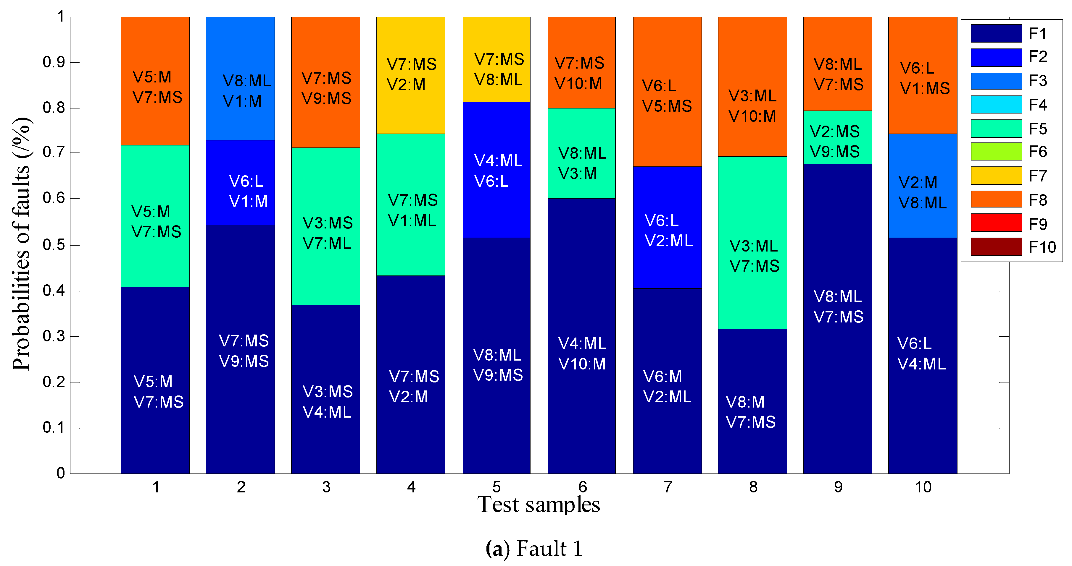
4.2.3. Fault Probability Analysis

The probability analysis scheme based FRBCSs proposed in Section 3.2 was utilized to identify the ten faults mentioned above. 600 samples were randomly selected from each fault state, as the experimental data (6000 samples in total).

Table 9. Comparison of the original accuracy and probability accuracy.

Faults	F1	F2	F3	F4	F5	F6	F7	F8	F9	F10	All Faults
Acc-original	0.80	0.65	0.58	0.94	0.58	0.77	0.71	0.62	0.71	0.85	0.72
Acc-p2	0.87	0.78	0.76	1.00	0.84	0.89	0.86	0.79	0.86	0.95	0.86
Acc-p3	0.92	0.94	0.88	1.00	0.96	1.00	0.94	0.90	1.00	1.00	0.95

is the comparison between original accuracy and probability accuracy for all faults, in which, Acc-original is the original accuracy of MPQEA-FRBCS, Acc-pi (i = 2, 3) represents the accuracy that the real fault can be found in the first i sequences. It is obvious that the accuracy has significant improvement with the increase of sorting numbers, it is verified the feasibility of the proposed probability analysis scheme.

The six sensor in offshore WT faults were taken to verify the feasibility of the probability analysis scheme with critical variables. A total of 60 test samples were randomly selected from the six faults, and the probabilistic fault analysis scheme mentioned in Section 3.2 was utilized to provide the probabilistic sorting of possible faults and corresponding interpretable description.

The experiment results of the fault probability analysis with critical variables are shown in Figure 8. In which variables V1~V10 respectively represent wind speed (y-axis), wind speed (z-axis), #2 pitch angle, wind speed (x-axis), generator rotor azimuth, generator torque, #3 pitch angle, yaw error, #1 pitch angle, and horizontal acceleration. The language labels (S, MS, M, ML, L) corresponded to Small, Middle Small, Middle, Middle Large, and Large.

In Figure 8, each test result outputs the three most likely faults in probabilistic form, and provides interpretable language labels of critical state variable. It can be seen that the real fault can be found in the range of the first three probability sorts in most test results. In this way, the reparation through probability sorting can shorten the time of fault troubleshooting, even if the fault identification result is unwarrantable. In addition, maintenance personnel can make more reasonable maintenance decisions by combining the probability sorting of faults, interpretable language labels of critical state variables, and expert knowledge.

5. Conclusions

In this study, an FRBCS based on the multi-population quantum evolutionary algorithm (MPQEA-FRBCS) is proposed to improve the identification accuracy of the operating states of WTs. A probabilistic fault identification strategy with interpretable critical variables is proposed to provide abundant and reliable reference information for maintenance personnel. The conclusions may be summarized as follows:

(1)

The proposed MPQEA-FRBCS can improve the classification performance of FRBCS in initial rule generation and rule set optimization. Hence, for the 18 well-known UCI data sets, MPQEA-FRBCS improves the average classification accuracy by 3.11% and 4.42% relative to FH-GBML-IVFS-Amp and GAGRAD, respectively.

(2)

The application of MPQEA-FRBCS to the operating state identification of offshore WTs improves the identification accuracy. From the comparison of the results with those of four other fault identification methods, MPQEA-FRBCS obviously improves identification accuracy by 6.73%, 8.83%, 12.46%, and 11.26%.

(3)

The proposed probabilistic fault identification scheme with interpretable critical variables can provide abundant and reliable reference information for maintenance personnel. The probability results of two and three sequences show 14% and 23% improvement in identification accuracy relative to the original accuracy of MPQEA-FRBCS, respectively. Meanwhile, the proposed fault identification scheme identifies the critical state variable of a fault to ensure interpretability.

References

1. Tchakoua, P.; Wamkeue, R.; Ouhrouche, M.; Slaouihasnaoui, F.; Tameghe, T.A.; Ekemb, G. Wind turbine condition monitoring: state-of-the-art review, new trends, and future challenges. Energies 2014, 7, 2595–2630. [Google Scholar] [CrossRef]
2. Tautz-Weinert, J.; Watson, S.J. Using scada data for wind turbine condition monitoring—A review. IET Renew. Power Gener. 2017, 11, 382–394. [Google Scholar] [CrossRef]
3. Chen, B.; Matthews, P.C.; Tavner, P.J. Automated on-line fault prognosis for wind turbine pitch systems using supervisory control and data acquisition. IET Renew. Power Gener. 2015, 9, 503–513. [Google Scholar] [CrossRef]
4. Deng, X.; Pan, Q.; Gao, Q. Research on the modeling and simulation of permanent magnet direct-driven wind turbine rotor imbalance fault. Power Syst. Prot. Control 2018, 46, 35–40. [Google Scholar]
5. Asian, S.; Ertek, G.; Haksoz, C.; Pakter, S.; Ulun, S. Wind turbine accidents: a data mining study. IEEE Syst. J. 2017, 11, 1567–1578. [Google Scholar] [CrossRef]
6. Quan, Z.; Xiong, T.; Wang, M.; Xiang, C.; Xu, Q. Diagnosis and early warning of wind turbine faults based on cluster analysis theory and modified ANFIS. Energies 2017, 10, 898. [Google Scholar]
7. Mojallal, A.; Lotfifard, S. Multi-physics graphical model-based fault detection and isolation in wind turbines. IEEE Trans. Smart Grid 2017, 99, 1–10. [Google Scholar] [CrossRef]
8. Laouti, N.; Othman, S.; Alamir, M. Combination of model-based observer and support vector machines for fault detection of wind turbines. Int. J. Autom. Comput. 2014, 11, 274–287. [Google Scholar] [CrossRef]
9. Cho, S.; Gao, Z.; Moan, T. Model-based fault detection, fault isolation and fault-tolerant control of a blade pitch system in floating wind turbines. Renew. Energy 2018, 120, 1–10. [Google Scholar] [CrossRef]
10. Bi, R.; Zhou, C.; Hepburn, D.M. Detection and classification of faults in pitch-regulated wind turbine generators using normal behavior models based on performance curves. Renew. Energy 2017, 105, 674–688. [Google Scholar] [CrossRef]
11. Zhang, D.; Qian, L.; Mao, B.; Huang, C.; Si, Y. A data-driven design for fault detection of wind turbines using random forests and XGboost. IEEE Access 2018, 6, 21020–21031. [Google Scholar] [CrossRef]
12. Colone, L.; Reder, M.; Tautz-Weinert, J.; Melero, J.J.; Natarajan, A.; Watson, S.J. Optimization of data acquisition in wind turbines with data-driven conversion functions for sensor measurements. Energy Procedia 2017, 137, 571–578. [Google Scholar] [CrossRef]
13. Chen, B.; Matthews, P.C.; Tavner, P.J. Wind turbine pitch faults prognosis using a-priori knowledge-based anfis. Expert Syst. Appl. 2014, 40, 6863–6876. [Google Scholar] [CrossRef]
14. Hu, R.L.; Leahy, K.; Konstantakopoulos, I.C.; Auslander, D.M.; Spanos, C.J.; Agogino, A.M. Using domain knowledge features for wind turbine diagnostics. In Proceedings of the 15th IEEE International Conference on Machine Learning and Applications, Anaheim, CA, USA, 18–20 December 2016. [Google Scholar]
15. Wang, Y.; Ma, X.; Qian, P. Wind turbine fault detection and identification through pca-based optimal variable selection. IEEE Trans. Sustain. Energy 2018, 99, 1–9. [Google Scholar] [CrossRef]
16. Ruiz, M.; Mujica, L.E.; Alférez, S. Wind turbine fault detection and classification by means of image texture analysis. Mech. Syst. Signal Process. 2018, 107, 149–167. [Google Scholar] [CrossRef] [Green Version]
17. Pashazadeh, V.; Salmasi, F.R.; Araabi, B.N. Data driven sensor and actuator fault detection and isolation in wind turbine using classifier fusion. Renew. Energy 2017, 80, 151–158. [Google Scholar] [CrossRef]
18. Paternain, D.; Bustince, H.; Pagola, M. Capacities and overlap indexes with an application in fuzzy rule-based classification systems. Fuzzy Sets Syst. 2016, 305, 70–94. [Google Scholar] [CrossRef]
19. Derhami, S.; Smith, A.E. A technical note on the paper “hga: hybrid genetic algorithm in fuzzy rule-based classification systems for high-dimensional problems”. Appl. Soft Comput. 2016, 41, 91–93. [Google Scholar] [CrossRef]
20. Prusty, M.R.; Jayanthi, T.; Chakraborty, J.; Seetha, H.; Velusamy, K. Performance analysis of fuzzy rule based classification system for transient identification in nuclear power plant. Ann. Nucl. Energy 2015, 76, 63–74. [Google Scholar] [CrossRef]
21. Chen, S.M.; Hsin, W.C. Weighted fuzzy interpolative reasoning based on the slopes of fuzzy sets and particle swarm optimization techniques. IEEE Trans. Cybern. 2017, 45, 1250–1261. [Google Scholar] [CrossRef] [PubMed]
22. Zare, M.; Koch, M. Groundwater level fluctuations simulation and prediction by ANFIS-and hybrid wavelet-ANFIS/ fuzzy c-means (FCM) clustering models: application to the Miandarband plain. J. Hydro-Environ. Res. 2017, 18, 63–76. [Google Scholar] [CrossRef]
23. Zhang, Y.X.; Qian, X.Y.; Peng, H.D.; Wang, J.H. An allele real-coded quantum evolutionary algorithm based on hybrid updating strategy. Comput. Intell. Neurosci. 2016, 9, 50–58. [Google Scholar] [CrossRef] [PubMed]
24. Layeb, A. A hybrid quantum inspired harmony search algorithm for 0-1 optimization problems. J. Comput. Appl. Math. 2013, 253, 14–25. [Google Scholar] [CrossRef]
25. Kuhne, P.; Poschke, F.; Schulte, H. Fault estimation and fault-tolerant control of the fast NREL 5-MW reference wind turbine using a proportional multi-integral observer. Int. J. Adapt. Control Signal Process. 2017, 32, 568–585. [Google Scholar] [CrossRef]
26. Zanon, A.; De Gennaro, M.; Kühnelt, H. Wind energy harnessing of the NREL 5 MW reference wind turbine in icing conditions under different operational strategies. Renew. Energy 2018, 115, 760–772. [Google Scholar] [CrossRef]
27. Odgaard, P.F.; Stoustrup, J.; Kinnaert, M. Fault-tolerant control of wind turbines: A benchmark model. IEEE Trans. Control Syst. Technol. 2012, 45, 313–318. [Google Scholar]
28. Abdelghaffar, H.M.; Woolsey, C.A.; Rakha, H.A. Comparison of three approaches to atmospheric source localization. J. Aerosp. Inf. Syst. 2017, 14, 40–52. [Google Scholar] [CrossRef]
29. Palma-Mendoza, R.J.; Rodriguez, D.; De-Marcos, L. Distributed relieff-based feature selection in spark. Knowl. Inf. Syst. 2018, 19, 1–20. [Google Scholar] [CrossRef]
30. Urbanowicz, R.J.; Meeker, M.; Cava, W.; Olson, R.S.; Moore, J.H. Relief-based feature selection: introduction and review. J. Biomed. Inf. 2018, 85, 189–203. [Google Scholar] [CrossRef]
31. Bache, K.; Lichman, M. UCI Machine Learning Repository. Available online: http://archive.ics.uci.edu/ml/datasets.html (accessed on 4 March 2019).
32. Sanz, J.A.; Galar, M.; Jurio, A.; Brugos, A.; Pagola, M.; Bustince, H. Medical diagnosis of cardiovascular diseases using an interval-valued fuzzy rule-based classification system. Appl. Soft Comput. 2014, 20, 103–111. [Google Scholar] [CrossRef]
33. Dombi, J.; Gera, Z. Rule based fuzzy classification using squashing functions. J. Intell. Fuzzy Syst. 2008, 19, 3–8. [Google Scholar]
34. Maesono, Y.; Moriyama, T.; Lu, M. Smoothed nonparametric tests and approximations of p-values. Ann. Inst. Stat. Math. 2017, 70, 969–982. [Google Scholar] [CrossRef]
Figure 1. Fuzzy partition of state variables.
Energies 12 02046 g001
Figure 2. Quantum coding of state rules for offshore WTs.
Energies 12 02046 g002
Figure 3. Flow chart of fuzzy rules mining based on MPQEA.
Energies 12 02046 g003
Figure 4. The sensor positions in the WT model.
Energies 12 02046 g004
Figure 5. Flow chart of fault identification and probability analysis for offshore WTs.
Energies 12 02046 g005
Figure 6. The weight sorting of WT features by ReliefF algorithm.
Energies 12 02046 g006
Figure 7. Comparison of confusion matrixes of the considered algorithms.
Energies 12 02046 g007aEnergies 12 02046 g007b
Figure 8. Probability analysis of the sensor faults in offshore WTs.
Energies 12 02046 g008aEnergies 12 02046 g008bEnergies 12 02046 g008c