5.1.1. Case Illustration and Wind Speed Samples
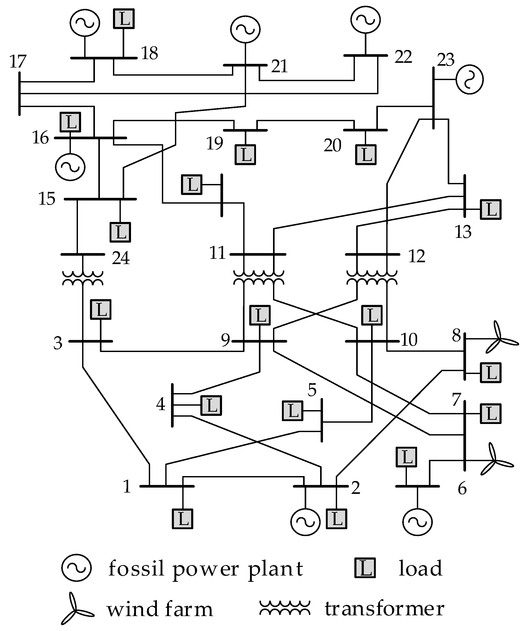
This paper uses a modified IEEE 24-node power system [
25] for example analysis, which is shown in
Figure 2. To verify the effectiveness of the algorithm, two wind farms are added to node 7 and 8, respectively. Supposing the wind speeds of node 7 and 8 obey normal distribution, the expectations of which are 8 m/s and 9 m/s and variances are 2 m/s and 2.2 m/s. The correlation coefficient of wind speed in node 7 and 8 is 0.99. Generally, the higher correlation coefficient of wind speed in different wind farms is, the variation trend would be more similar in these wind farms, which is to say that if the wind speed in node 7 is huge, then the wind speed in node 8 would be huge also. Therefore, if we choose the correlation coefficient of wind speed in node 7 and 8 as 0.99, which is a strong correlation relationship, then the voltage fluctuation of the power system is the most serious under this circumstance, as the system voltage average beyond limits would be more likely to occur. According to the wind speed joint distribution of nodes 7 and 8, 8000 wind speed samples are generated randomly in each wind farm. The power factor of the wind turbine is 0.98, the rated, cut-in and cut-out wind speed of the wind turbine is 15 m/s, 3 m/s and 25 m/s, respectively. Considering the rated, cut-in and cut-out wind speeds, the active and reactive power of the wind turbine can be calculated using Equations (1) and (2) according to wind speed. In reality, the uncertainty of the load is much less than that of wind speed, so we did not take the uncertainty of the load into consideration, and regard them as determined values.
5.1.2. Effectiveness Verification of the Proposed Method
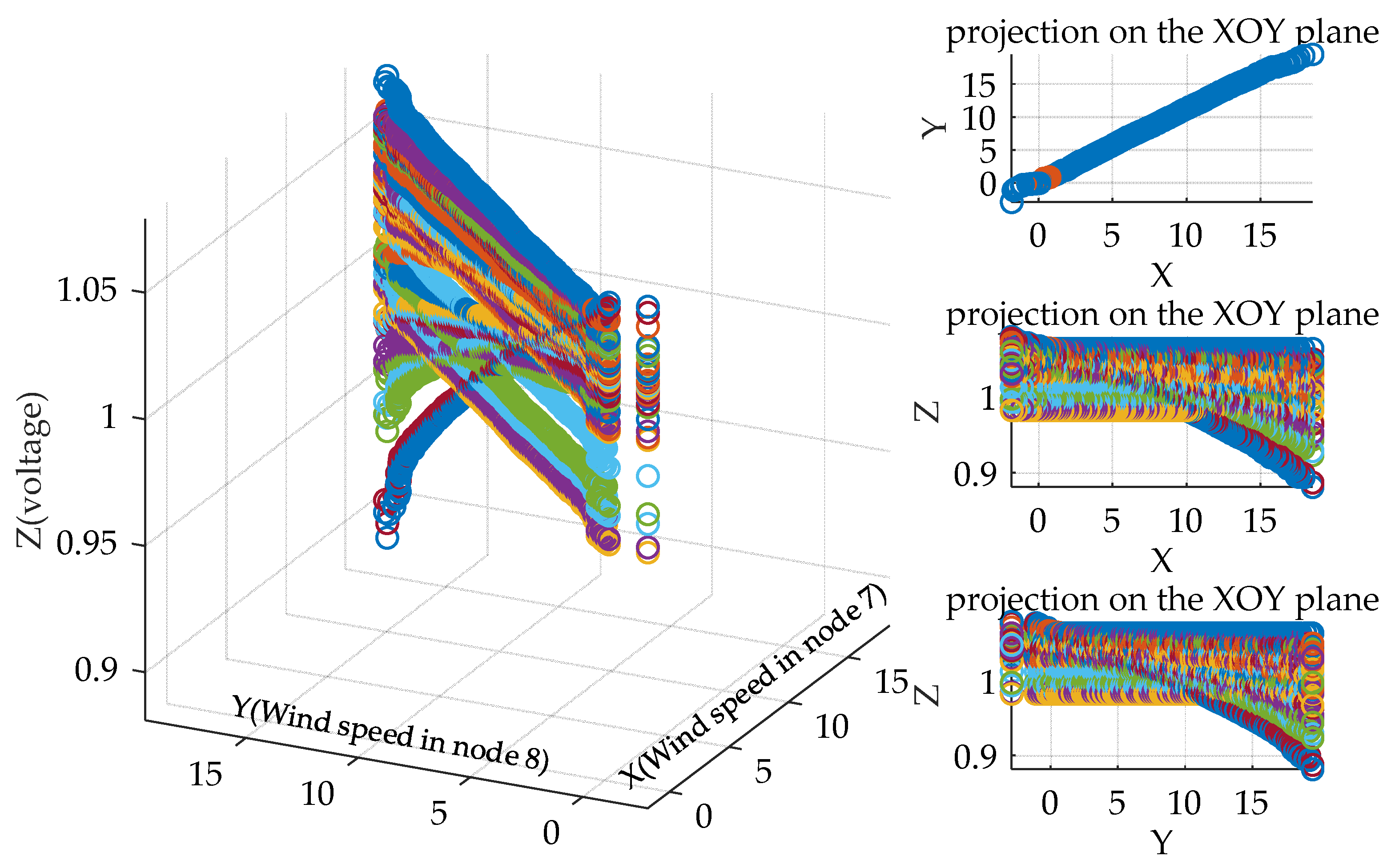
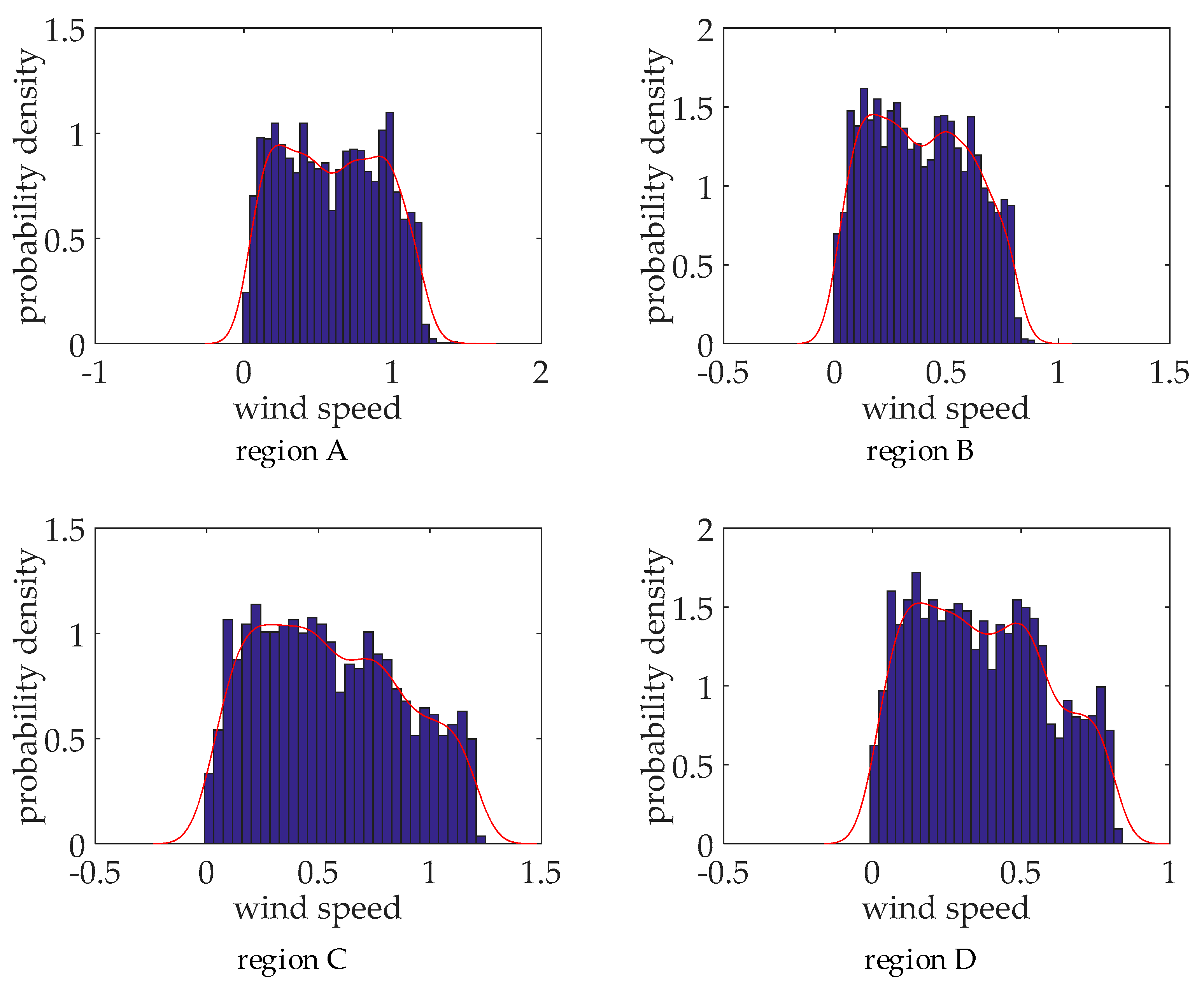
According to the 8000 generated wind speeds in
Section 5.1.1, non-parametric kernel density estimation is used to obtain the probability density function of these wind speed samples, and their joint probability density function is shown in
Figure 3. In this figure, the
x-z and
y-z planes denote the probability density function of wind speed in node 7, respectively. Apparently, the probability density function of wind speed in nodes 7 and 8 obey normal distribution because the sample number is huge, which verifies the effectiveness of using non-parametric kernel density estimation to obtain the probability density function of wind speed. In this case, we suppose that the wind speeds in node 7 and 8 obey the normal distribution in
Section 5.1.1. Therefore, we select the normal copula function to establish their wind speed joint distribution model; the copula function and the joint probability density function solved through this copula are shown in
Figure 4.
In order to verify the validity of joint probability density function in
Figure 4, we design a method that calculates the similarity of joint probability density function between
Figure 3 and
Figure 4. Extract
R x-axis and
y-axis coordinates randomly in
Figure 3 and
Figure 4, and let their
z-axis coordinates are
and
, where
i = 1, 2,…,
R,
j = 1, 2,…,
R. Calculate the error using the formula in Equation (25), the smaller error is, the more similar joint probability density function between
Figure 3 and
Figure 4 is. Let
R = 500, 1000, 1500, 2000, 2500, and the average error and maximum error of probability density in
Figure 3 and
Figure 4 are shown in
Table 2. We can see the errors under different
R values are small enough, which verifies that the joint probability density function in
Figure 4 is basically the same as that in
Figure 3, and this illustrates that vine-copula could effectively construct a joint probability density of multi-dimensional random variables.
Monte Carlo sampling is used in the copula-based joint probability density function to generate 10,000 wind speed samples, and the Rosenblatt transform is used to convert the correlated wind speed samples to independent wind speed samples. On this basis, we calculate node voltage using the probabilistic load flow based on the semi-invariant method (shorthand as proposed method), and the node voltage results are shown in
Figure 5. In order to verify the effectiveness of this copula and the semi-invariant based probabilistic load flow calculation in this paper, we use the Monte Carlo method to sample wind speed data in
Section 5.1.1 for 10,000 times (simplified Monte Carlo method), and uses these wind speed samples to calculate power load for 10,000 times (detailed Monte Carlo method). The average error and maximum error of the proposed method and Monte Carlo method are shown in
Table 3. From this Table, the calculation results of the proposed and the Monte Carlo method are basically consistent, and this illustrates that the proposed method is effective in the statistical characteristics of the output variables.
In order to verify the accuracy of the proposed method in the probability distribution characteristics of the output variables further. Taking the voltage amplitude of node 3 and node 4, the active power of branches 21-15 and 3-1, and the reactive power of branch 19-16 and 23-20 as examples, this paper calculates their distribution function using the proposed method and Monte Carlo method. The distribution functions are shown in
Figure 6. From this figure, the distribution curve of these two methods are close to each other. Through verification, the distribution function of output variables in other nodes or branches using these two methods are very similar, and the maximum relative error is 2.14%, which illustrates that the proposed method could accurately obtain probability distributions, and further proves that the proposed method has higher precision.
In order to verify the novelty of the study compared with other studies, the traditional three point estimate method taking no account of wind speed correlation in [
26] (traditional three point estimate method), and the three point estimate method considering wind speed correlation in [
19] (improved three point estimate method) are used to sample wind speed. Then, the expectation and standard deviation of voltage amplitude and phase angle with Monte Carlo method are compared. Together with the proposed method, the average error of these three methods and the Monte Carlo method are shown in
Table 4. In this table, the error of the traditional three point estimate method is the largest among the three method. The reason lies in that this method take no account of wind speed correlation, which has a significant influence on the calculation results. The improved three point estimate method takes wind speed correlation into consideration, but the error is still larger than the proposed method in this paper. The method only uses the correlation coefficient as the description index of the correlation of wind speeds. In the actual situation, the correlation between wind speeds is complex and variable. Therefore, it is difficult to fully describe the relationship between these wind speeds. In fact, the linear correlation coefficient, Spearman correlation coefficient [
27,
28] etc. cannot fully describe the correlation between random variables; copula-based joint probability distribution is the best description.


