A Vine-Copula Based Voltage State Assessment with Wind Power Integration

Abstract

With the increasing rate of wind power installed capacity, voltage state assessment with large-scale wind power integration is of great significance. In this paper, a vine-copula based voltage state assessment method with large-scale wind power integration is proposed. Firstly, the nonparametric kernel density estimation is used to fit the wind speed distribution, and vine-copula is used to construct the wind speed joint distribution model of multiple regions. In order to obtain voltage distribution characteristics, probabilistic load flow based on the semi-invariant method and wind speed independent transformation based on the Rosenblatt transformation are described. On this basis, a voltage state assessment index is established for the more comprehensive evaluation of voltage characteristics, and a voltage state assessment procedure is proposed. Taking actual wind speed as an example, the case study of the IEEE 24-node power system and the east Inner Mongolia power system for voltage state assessment with large-scale wind power integration are studied. The simulation results verify the effectiveness of the proposed voltage state assessment method.

1. Introduction

In recent years, the growth rate of wind power installed capacity has been rapid [1]. However, the consumption of wind power has restricted its development seriously [2]. Both the randomness and volatility of wind power have a great impact on the operation of a system [3], especially with respect to the problem of voltage beyond limits. In addition, there is a complex correlation of wind speed in different regions, especially a positive correlation [4,5], which causes serious voltage fluctuation problems. Therefore, the study of voltage state assessment with large-scale wind power integration is of great significance, and we must consider the uncertainty and correlation of wind speed in different regions.

In this paper, we firstly apply the vine-copula function to the voltage state assessment method with large-scale wind power integration. Therefore, the characteristics of the vine-copula function are discussed in the introduction.

The vine-copula function is an improved algorithm of the copula function. The copula function is an effective tool for constructing a joint probability distribution of multi-dimensional random variables [6]. It is actually a function that connects the joint distribution function of variables with their respective edge distribution functions. The related theory could be traced back to 1959, when Sklar linked the multivariate edge distribution using the copula function. In the 1990s, the copula function was used in the financial field [7], and in recent years the copula function has been applied to the study of power systems such as the probabilistic optimal power flow [8], probabilistic power flow [9] and risk assessment [10].

However, the traditional copula model could only describe the nonlinearity, asymmetry and tail correlation between two random variables, and building higher-dimensional copula is generally recognised as a difficult problem. Limited by this reason, vine-copula was proposed by Kjersti Aas [11]. In [11], a pair-copula decomposition is used in the vine-copula function, which is represented a more flexible and intuitive way of extending bivariate copula to higher dimensions. Multivariate data exhibiting complex patterns of dependence in the tails could be modelled using the vine-copula function. This function allows inference on the parameters of the pair-copulae on various levels of the construction. This construction is hierarchical in nature, the various levels standing for growing conditioning sets, incorporating more variables.

The paper is organized as follows. A literature review is presented in Section 2. The output power model of a wind farm, the wind speed distribution model of a region and wind speed joint distribution model of multiple regions are presented in Section 3. In Section 4, a probabilistic load flow based on the semi-invariant method and wind speed independent transformation based on the Rosenblatt transformation are described first. Then, a voltage state assessment index is established, and a voltage state assessment procedure is proposed. Section 5 provides the case study of IEEE 24-node power system and the east Inner Mongolia power system for voltage state assessment with large-scale wind power integration, the simulation results are presented to verify the effectiveness of the proposed voltage state assessment method.

2. Literature Review

The voltage state assessment method with large-scale wind power integration can be divided into two processes, namely: (1) modelling correlated random variables; and (2) voltage stability assessment using the above model. In the literature review section, we review the existing studies in the context of these two aspects.

In the field of modelling correlated random variables, scholars have developed a great amount of work. Until now, common models have included the edge distribution model based on the correlation coefficient, and the joint distribution model based on the copula function. In the study of the edge distribution model based on the correlation coefficient, Yang H. et al. [12] propose a third-order polynomial normal transformation method to transform multivariate non-normal dependent random variables to standard normal independent ones. Zou B. et al. [13] propose a ninth-order polynomial normal transformation. These two correlation models are based on the linear correlation coefficient, which is not suitable for describing a nonlinear correlated relationship. The complete representation of random variable correlation characteristics is the joint probability distribution [8]. Besides, the acquisition of correlation coefficient is based on practical experience, and the credibility is not high. Furthermore, the model only uses the correlation coefficient as the description of random variables’ correlation. In actual conditions, the correlation between the wind speeds in different regions is complex and changeable; thus it is difficult to completely describe the relationship between wind speeds in multiple regions using this model.

The joint distribution model based on the copula function does not require a correlation coefficient matrix of random variables in advance, but uses the copula function as the link to describe the correlated relationship between random variables completely [14]. Xie Z. et al. [8] use copula to deal with correlations of wind speed. Widen J. et al. [9] use a Gaussian copula to deal with correlated samplings for an arbitrary set of distributed PV systems. These copula-based joint distribution models are especially suited for describing correlated relationship with two random variables. If the number of random variables exceed three, there would be a dimension disaster, and copula functions cannot describe a correlated relationship with high accuracy. For example, if the dimension is d, and there are n data dots in each dimension, then a copula based joint distribution would be generated using n^d data dots; when n exceeds 1000 in general, when d ≥ 3, the data amount would be too huge for computation. In recent years, the vine-copula function is introduced to establish a joint distribution model of high-dimensional random variables, and some scholars use it to calculate probabilistic or probabilistic optimal power flow. Thesis [15] proposes an improved point estimate method based on pair-copula and probability integral transformation for probabilistic power flow calculation. However, this method could only calculate the expectation and variance of the power flow results, but cannot obtain its distribution characteristics, so this method is hard to use for voltage state assessment.

Voltage stability is of great significance to the safe operation of a power system, and voltage state assessment is a hot topic of research and discussion. Thesis [16] proposes a static voltage stability index for evaluating the severity of the loading situation, which is used for predicting voltage instability at a definite load value. Thesis [17] proposes a curve based voltage stability assessment method, and implements a visualization framework for assessing voltage stability margins. Thesis [18] studies the effects on voltage stability of the integration of a wind farm into the electricity grid. With the large capacity of wind power installed in modern power system, traditional voltage state assessment methods are hard to apply, and using these methods, it is especially hard to deal with the randomness and correlation of wind power. Therefore, this paper proposes a vine-copula based voltage state assessment method with large-scale wind power integration. This method uses the vine copula function to first establish a wind speed joint distribution model of multiple regions, and calculates probabilistic load flow to evaluate the voltage state. To resolve the problem that a semi-invariant based probabilistic load flow method cannot deal with correlated random variables, this paper uses the Rosenblatt transformation to transform the correlated wind speed variables to independent variables, and proposes a voltage state assessment procedure.

3. Wind Speed Joint Distribution Model in Multiple Regions

In this section, the output power model of a wind farm is described. Then, a wind speed distribution model of a region and wind speed joint distribution model of multiple regions are established.

3.1. Output Power Model of a Wind Farm

In power system stability analysis, a large-scale wind farm with multiple wind turbines is usually equivalent to one equivalent machine [19]. For a single wind turbine, the wind speed determines its active output. The corresponding relationship is as follows [19]:

$$P_w(v)=\{\begin{array}{ll}0\hfill & v\le v_{ci},v\ge v_{co}\\ P_r\frac{v-v_{ci}}{v_r-v_{ci}}\hfill & v_{ci}\le v\le v_r\\ P_r\hfill & v_r\le v\le v_{co}\end{array}$$

(1)

where v is wind speed; P_w(v) is the active output of wind farm under wind speeds v, v_ci, v_r; and v_co is the cut-in wind speed, rated wind speed and cut-out wind speed of the equivalent machine in a wind farm, respectively. P_r is the rated output power of the equivalent machine in wind farm.

A large-scale wind farm with a coordinated control unit and reactive power compensation capability is able to adjust its reactive power output within a certain range. Constant power factor operation is the main mode of operation. Therefore, the reactive power of a wind farm is as follows,

$$Q_w(v)=P_w(v)\cdot \tan \phi$$

(2)

where Q_w(v) is the reactive output of wind farm under wind speed v, φ is the power factor angle.

3.2. Wind Speed Distribution Model of a Region

Wind energy is a clean and renewable energy. Wind speed is the main factor that determines the output of wind farms. In this paper, we suppose that the wind speed in a region obeys the same distribution, and different wind farms in a region use this wind speed as input. Nowadays, studies mostly use the Weibull distribution to describe the wind speed of a region [20]. However, the shape factor and scale factor of a Weibull distribution is hard to confirm accurately in different regions. Therefore, the best description of wind speed distribution is to use its actual data for probability statistics analysis. Non-parametric kernel density estimation makes no use of prior knowledge about data distribution, nor attaches any assumptions to the data distribution. This is a method to study the data distribution characteristics from data itself. Therefore, it is highly valued in statistical theory and more applied fields. In this paper, non-parametric kernel density estimation is applied to fit wind speed distribution using wind speed samples, and its expression is as follows:

$${\widehat{f}}_w(v)=\frac{1}{N}{\displaystyle \sum _{i=1}^N{K}_h(v-X_i)}$$

(3)

where K_h is the kernel function, N is the sequence capacity, X_i is the wind speed sample, i = 1, 2,…, N.

3.3. Wind Speed Joint Distribution Model of Multiple Regions

This paper uses the vine copula function to establish a wind speed joint distribution model of multiple regions. The core idea of vine copula is to decompose the joint distribution of multi-dimensional random variables into two-dimensional copula functions including their original and conditional variables.

Considering the wind speed random variables X = (X₁, X₂,…, X_N) in multiple regions, the probability density functions f_{1, 2,…, N}(x₁, x₂,…, x_N) can be decomposed as follows,

$$f_{1,2,\dots ,N}(x_1,x_2,\dots ,x_N)=f_1(x_1)f_{2|1}(x_2|x_1)f_{3|1,2}(x_3|x_1,x_2)\dots f_{N|1,2,\dots ,N-1}(x_N|x_1,x_2,\dots ,x_{N-1})$$

(4)

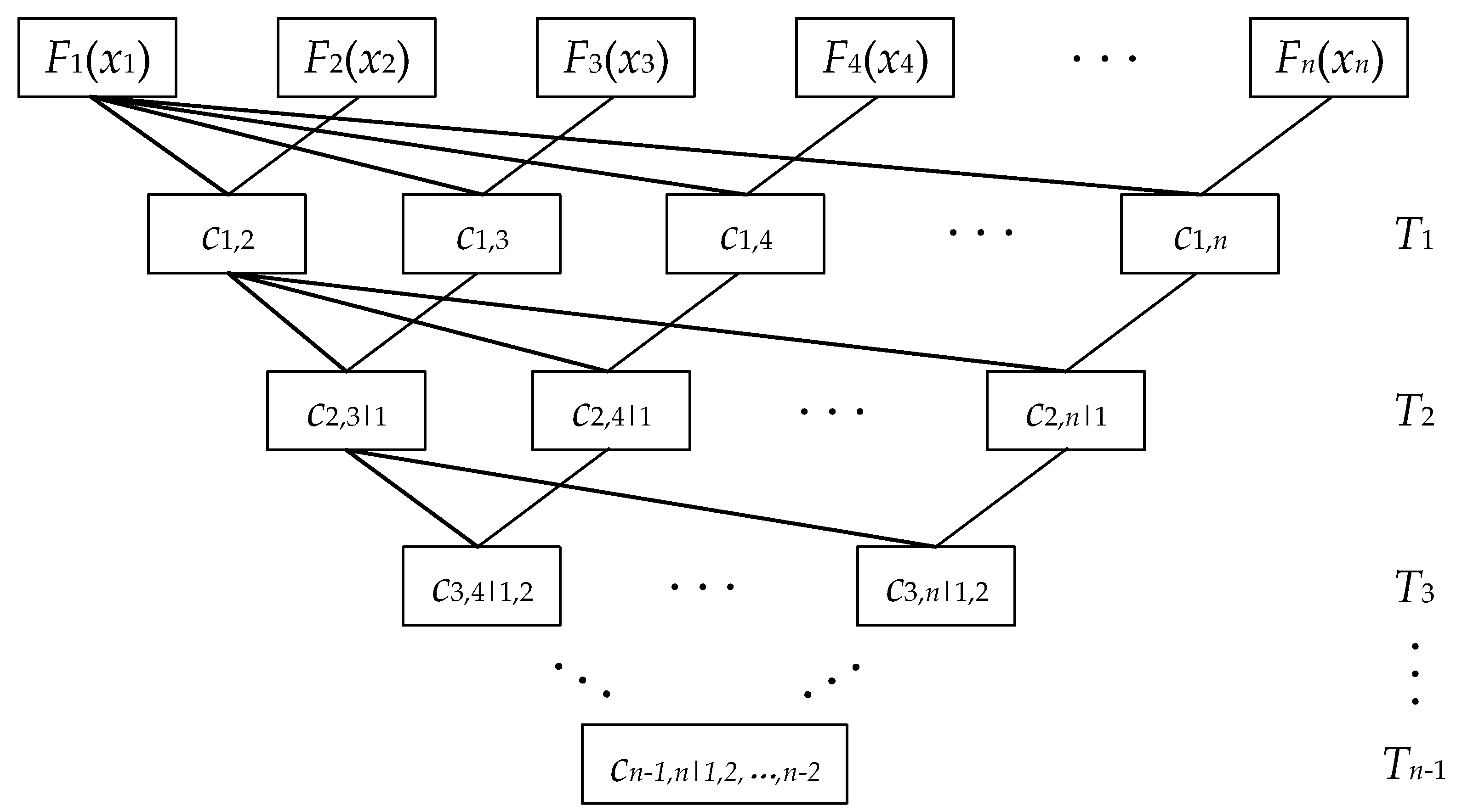
where f_k(x_k) denotes the probability density function of X_i, k = 1, 2,…, N, f_{k|1, 2,…, k−1}(x_k|x₁, x₂,…, x_k−1) denotes the condition probability density function, k = 2, 3,..., N. Equation (4) can be decomposed into many forms. Thesis [21] introduces the vine copula function to describe different decomposition methods. Common vine models include C-vine and D-vine. The structure of C-vine is shown in Figure 1, and this paper uses C-vine to decompose Equation (4). The decomposed expression is as follows,

$$f_{1,2,\dots ,N}(x_1,x_2,\dots ,x_N)={\displaystyle \prod _{k=1}^N{f}_k(x_k)}\cdot {\displaystyle \prod _{i=1}^{N-1}{\displaystyle \prod _{j=1}^{N-i}{c}_{i,i+j|1,\dots ,j-1}(F_{i|}{}_{1,2,\dots ,i-1}(x_i|x_1,\dots ,x_{i-1}),F_{i+j|}{}_{1,2,\dots ,i-1}(x_{i+j}|x_1,\dots ,x_{i-1}))}}$$

(5)

where F_k(x_k) denotes the edge cumulative distribution function of X_i, k = 1, 2,…, N, and F_{k|1, 2,…, k−1}(x_k|x₁, x₂,…, x_k−1) denotes conditional cumulative distribution function, k = 2, 3,..., N.

Vine copula is used to convert the joint probability density function of wind speed random variables into the edge probability density function of a region and a number of two-dimensional copula functions. Copula functions could be classified into an Ellipse function family (Ellipse-copula) and Archimedean function family (Archimedean-copula). Among them, the Elliptic function family includes the normal copula function and t copula function, and the Archimedean function family includes the gumbel copula function, clayton copula function and frank copula function [22]. Different copula functions have different function structures, and their tail characteristics are suitable for describing different dependent relationships. The probability density function and tail characteristics of different copula types are shown in

Table 1. Probability density function and tail characteristics of different copula types.

Copula	Probability Density Function	Tail Characteristics
Normal	$C_n(u,v|{\rho }_n)={\displaystyle {\int }_{-\infty }^{{\varphi }^{-1}(u)}{\displaystyle {\int }_{-\infty }^{{\varphi }^{-1}(v)}\frac{1}{2\pi \sqrt{1-{\rho }_n^2}}}}\cdot \exp (-\frac{s^2-2{\rho }_{n}sr+r^2}{2-2{\rho }_n^2})dsdr$	Symmetrical and progressively independent tail
t	$C_t(u,kv|{\rho }_t,k)={\displaystyle {\int }_{-\infty }^{{\varphi }^{-1}(u)}{\displaystyle {\int }_{-\infty }^{{\varphi }^{-1}(v)}\frac{1}{2\pi \sqrt{1-{\rho }_t^2}}}}\cdot {[1+\frac{s^2-2{\rho }_{t}sr+r^2}{2-2{\rho }_t^2}]}^{-(k+2)/2}dsdr$	Symmetrical tail
Gumbel	$C_g(u,v|{\rho }_g)=\exp \{-{[{(-\ln u)}^{{\rho }_g}+{(-\ln v)}^{{\rho }_g}]}^{1/{\rho }_g}\}$	Asymmetrical tail and sensitive to the upper tail
Clayton	$C_c(u,v|{\rho }_c)=\max [(u^{-{\rho }_c}+v^{-{\rho }_c}-1{)}^{-1/{\rho }_c},0]$	Asymmetrical tail and sensitive to the lower tail
Frank	$C_f(u,v|\alpha )=-\frac{1}{{\rho }_f}\ln [1+\frac{(e^{-u}-1)(e^{-v}-1)}{e^{-{\rho }_f}-1}]$	Symmetrical and progressively independent tail

.

This five type of copula functions have different tail characteristics. It is of great significance to find which type is more suitable to describe wind speed joint distribution. Before selecting the optimal copula function, the correlation coefficient ρ of each copula function need to be determined based on the initial sample. For the method of obtaining ρ, there are methods such as maximum likelihood estimation, distribution estimation, semi-parametric estimation and non-parametric estimation. This paper selects a widely used maximum likelihood estimation method, which is as follows:

$$L(\rho )={\displaystyle \sum \ln c(\widehat{f}(x_1),\widehat{f}(x_2))}$$

(6)

$$\widehat{\rho }=\arg \max L(\rho )$$

(7)

where $\widehat{f}(x_1)$ and $\widehat{f}(x_2)$ are edge distribution function of x₁ and x₂, which could be calculated using Equation (3), $\widehat{\rho }$ is the estimated value of correlation coefficient ρ, and the copula model can be obtained by bringing $\widehat{\rho }$ and raw data into the copula function in Table 1.

For selecting the optimal copula function, this paper compares the Euclidean distance of the empirical copula function and the evaluated copula function (including normal copula, t copula, gumbel copula, clayton copula and frank copula). The method of calculating the Euclidean distance is as follows,

$$d_{Eucl}={\displaystyle \sum _{t=1}^T\sqrt{{[x_A(t)-x_B(t)]}^2+{[y_A(t)-y_B(t)]}^2+{[z_A(t)-z_B(t)]}^2}}$$

(8)

where A denotes the evaluated copula function, B denotes the empirical copula function, T denotes the sample size, x, y and z denote three-dimensional coordinates.

4. Voltage State Assessment

In this section, probabilistic load flow based on the semi-invariant method and wind speed independent transformation based on the Rosenblatt transformation are described. Then, a voltage state assessment index is established, and a voltage state assessment procedure is proposed.

4.1. Probabilistic Load Flow Based on Semi-Invariant Method

In this paper, voltage state assessment is based on probabilistic load flow. Two main random factors considered in probabilistic load flow calculation include load and wind turbine output. Among them, the probabilistic model of load adopts the truncated normal distribution in [23], and we suppose the loads in different nodes are independent. The vine-copula model is adopted to describe the probabilistic characteristics of wind farm output.

The probabilistic load flow can be calculated using semi-invariant and Gram-Charlier series expansion methods, which linearize the load flow equation at a reference operation point, and obtain the sensitivity matrix of state vector (such as voltage) to random perturbation vector (such as power input). The linearization method of load flow equation at the reference operation point is as follows:

$$V=V_0+\Delta V=V_0+S_0\cdot \Delta W$$

(9)

where V denotes the node voltage vector, V₀ denotes the node voltage vector at reference operation point, $\Delta V$ denotes the node voltage change vector, S₀ denotes the sensitivity matrix of voltage to power input, $\Delta W$ denotes the random perturbation vector of power input in different nodes.

Equation (9) is a linear transformation of the random variables. The distribution of $\Delta V$ could be obtained from the distribution of $\Delta W$ by convolution calculation. Assuming that the random perturbation vector of power input ($\Delta W$) in different nodes is independent (we have already suppose the load in different nodes are independent, so random perturbation vector of load is in different nodes are independent, although wind speed and wind farm output are correlated, we would transform them to independent random variable in Section 3.2), convolution could be reduced to a few semi-invariant algebra operations using the nature of the semi-invariant, and we will obtain the semi-invariants of $\Delta V$ in different orders. After that, the probability density function of the state variables could be calculated by using the Gram-Charlier series expansion. Let ${\gamma }_{\Delta V}^{(k)}$ denote k-order semi-invariant of $\Delta V$, then the probability density function and distribution function could be expressed as follows using Gram-Charlier series expansion,

$$f_{\Delta V}(\Delta V)=\varphi (\Delta V)+\frac{A_1\cdot {\varphi }^{(1)}(\Delta V)}{1!}+\frac{A_2\cdot {\varphi }^{(2)}(\Delta V)}{2!}+\dots +\frac{A_n\cdot {\varphi }^{(n)}(\Delta V)}{n!}$$

(10)

$$F_{\Delta V}(\Delta V)={\displaystyle {\int }_{-\infty }^{+\infty }[\varphi (\Delta V)+\frac{A_1\cdot {\varphi }^{(1)}(\Delta V)}{1!}+\frac{A_2\cdot {\varphi }^{(2)}(\Delta V)}{2!}+\dots +\frac{A_n\cdot {\varphi }^{(n)}(\Delta V)}{n!}]d\Delta V}$$

(11)

where $\varphi (•)$ denotes probability density function of standard normal distribution, ${\varphi }^{(n)}(\Delta V)$ is the n-order derivative of $\varphi (•)$, A₁, A₂,…, A_n denote the coefficients of the Gram-Charlier series, which are expressed as follows (we only show the first eight orders and this could meet the engineering accuracy requirements),

$$\{\begin{array}{ll}{A}_1=0& A_5=-{\gamma }_{\Delta V}^{(5)}\\ A_2=2& A_6={\gamma }_{\Delta V}^{(6)}+10{({\gamma }_{\Delta V}^{(3)})}^2\\ A_3=-{\gamma }_{\Delta V}^{(3)}& A_7=-({\gamma }_{\Delta V}^{(7)}+35{\gamma }_{\Delta V}^{(3)}{\gamma }_{\Delta V}^{(4)})\\ A_4={\gamma }_{\Delta V}^{(4)}& A_8={\gamma }_{\Delta V}^{(8)}+56{\gamma }_{\Delta V}^{(3)}{\gamma }_{\Delta V}^{(5)}+35{({\gamma }_{\Delta V}^{(4)})}^2\end{array}$$

(12)

4.2. Wind Speed Independent Transformation

The wind speed joint distribution model in Section 3.3 describes the correlation among the wind speed in different regions. However, the probabilistic load flow calculation based on semi-invariant method requires input variables to be independent. Therefore, the wind speed with correlation needs to be transformed into independent variables. The commonly used methods are Rackwitz-Fiessler transformation, Nataf transformation and Rosenblatt transformation [24]. Among them, Rackwitz-Fiessler transformation assumes that the correlation between variables is unchangeable, or ignores the change in correlation, which would result in large errors. Nataf transformation uses a correlation coefficient matrix to describe the correlation relationship, which cannot capture the nonlinear relationship between variables. When the variables do not obey the normal distribution, the method may lead to a large error. The Rosenblatt transformation is a method to transform a set of non-normal correlated/non-correlated random variables into a set of equivalent normal independent random variables, and this method is not easily affected by the type of variable distribution and whether the correlation is linear or not. This paper selects the Rosenblatt transformation to transform the correlated wind speed into independent variables.

As for wind speed random variables X = (X₁, X₂,…, X_N) in multiple regions, assuming that the joint cumulative distribution function is F_{1, 2,…, N}(x₁, x₂,…, x_N), Besides, another set of independent standard normal variable Y = (Y₁, Y₂,…, Y_N). The relationship between X and Y is as follows:

$$\{\begin{array}{l}\varphi (y_1)=F_1(x_1)\hfill \\ \varphi (y_2)=F_{2|1}(x_2|x_1)\hfill \\ \cdots \hfill \\ \varphi (y_N)=F_{N|1,2,\dots ,N}(x_N|x_1,x_2,\dots ,x_N)\hfill \end{array}$$

(13)

Invert Equation (13), an independent standard normal variable Y can be obtained, which is expressed as follows:

$$\{\begin{array}{l}{y}_1={\varphi }^{-1}[F_1(x_1)]\hfill \\ y_2={\varphi }^{-1}[F_{2|1}(x_2|x_1)]\hfill \\ \cdots \hfill \\ y_N={\varphi }^{-1}[F_{N|1,2,\dots ,N-1}(x_N|x_1,x_2,\dots ,x_{N-1})]\hfill \end{array}$$

(14)

Equation (14) is called the Rosenblatt transformation. Through this transformation, the correlated wind speed random variables are transformed to independent standard normal random variables. The Rosenblatt inverse transform of Equation (13) is as follows:

$$\{\begin{array}{l}{x}_1=F_1^{-1}[\varphi (y_1)]\hfill \\ x_2=F_{2|1}^{-1}[\varphi (y_2)|x_1]\hfill \\ \cdots \hfill \\ x_N=F_{N|1,2,\dots ,N-1}^{-1}[\varphi (y_N)|x_1,x_2,\dots ,x_{N-1}]\hfill \end{array}$$

(15)

The expression of $F_{i|1,2,\dots ,i}(x_i|x_1,x_2,\dots ,x_i)$ could be calculated using recursion, where i = 1, 2,…, N. Using Equation (5) and Equation (6), let N = 2, we know that:

$$f_{2|1}(x_2|x_1)=\frac{f_{1,2}(x_1,x_2)}{f_1(x_1)}=\frac{c_{1,2}\cdot f_1(x_1)\cdot f_2(x_2)}{f_1(x_1)}=c_{1,2}\cdot f_2(x_2)$$

(16)

$$F_{2|1}(x_2|x_1)={\displaystyle {\int }_{-\infty }^{x_2}{f}_{2|1}(x_2|x_1)}d{x}_2={\displaystyle {\int }_{-\infty }^{x_2}{c}_{1,2}\cdot f_2(x_2)d{x}_2}$$

(17)

Next, Using Equation (5), Equation (6) and Equation (16), let N = 3, we know that:

$$f_{3|1,2}(x_3|x_1,x_2)=\frac{f_{1,2,3}(x_1,x_2,x_3)}{f_1(x_1)\cdot f_{2|1}(x_2|x_1)}=\frac{c_{1,2}\cdot c_{1,3}\cdot c_{2,3|1}\cdot f_1(x_1)\cdot f_2(x_2)\cdot f_3(x_3)}{f_1(x_1)\cdot c_{1,2}\cdot f_2(x_2)}=c_{1,3}\cdot c_{2,3|1}\cdot f_3(x_3)$$

(18)

$$F_{3|1,2}(x_3|x_1,x_2)={\displaystyle {\int }_{-\infty }^{x_3}{f}_{3|1,2}(x_3|x_1,x_2)}d{x}_2={\displaystyle {\int }_{-\infty }^{x_3}{c}_{1,3}\cdot c_{2,3|1}\cdot f_3(x_3)d{x}_3}$$

(19)

Using this method, we could deduce the expression of $F_{i|1,2,\dots ,i}(x_i|x_1,x_2,\dots ,x_i)$ [24], where I = 1, 2,…, N,

$$\{\begin{array}{l}{F}_1(x_1)={\displaystyle {\int }_{-\infty }^{x_1}{f}_1(x_1)d{x}_1}\hfill \\ F_{2|1}(x_2|x_1)={\displaystyle {\int }_{-\infty }^{x_2}{c}_{1,2}{f}_2(x_2)d{x}_2}\hfill \\ ⋮\hfill \\ F_{i|1,2,\dots ,i}(x_i|x_1,x_2,\dots ,x_i)={\displaystyle {\int }_{-\infty }^{x_i}{c}_{1,i}{c}_{2,i|1}\cdots c_{i-1,i|1,2,\dots ,i-2}{f}_i(x_i)d{x}_i}\hfill \\ ⋮\hfill \\ F_{N|1,2,\dots ,N}(x_N|x_1,x_2,\dots ,x_N)={\displaystyle {\int }_{-\infty }^{x_N}{c}_{1,N}{c}_{2,N|1}\cdots c_{N-1,N|1,2,\dots ,N-2}{f}_N(x_N)d{x}_N}\hfill \end{array}$$

(20)

The Rosenblatt transformation establishes the link relationship between correlated wind speed random variables and independent standard normal variables. We could use some sampling method to select some wind speed variables first, and transform them to independent standard normal variables using Equation (14).

4.3. Voltage State Assessment Method

4.3.1. Voltage State Assessment Index

In order to evaluate the voltage state comprehensively and accurately, three indexes are defined, including system voltage average beyond limits probability, node voltage confidence interval and node voltage exponential entropy.

(1) System voltage average beyond limits probability.

In order to evaluate the voltage beyond limits situation with large-scale wind power integration, we need to take the voltage beyond limits situation of all nodes in the system into account. Assuming we have calculated power flow for K times, and we could know the times that the voltage of node i is out of range through defining qualified voltage interval, let it be k_i. and the voltage beyond limits probability of node i can be expressed as follows:

$$P_i^{\mathrm{beyond}}=\frac{k_i}{K}$$

(21)

Assuming there are S nodes in the system, and the system voltage average beyond limits probability can be expressed as follows:

$${\overline{P}}_{}^{\mathrm{beyond}}={\displaystyle \sum _{i=1}^S\frac{P_i^{\mathrm{beyond}}}{S}}$$

(22)

(2) Node voltage exponential entropy.

In order to evaluate the complexity of node voltage, exponential entropy is introduced. Firstly, we need to divide the voltage into L interval, which is $[{\tilde{V}}_{\min },{\tilde{V}}_1),[{\tilde{V}}_1,{\tilde{V}}_2),\dots ,[{\tilde{V}}_{L-1},{\tilde{V}}_{\max }]$. As for node i, count the number that V_i lies in each interval, which is $l_i^1,l_i^2,\dots ,l_i^L$ (assuming we have calculated power flow for K times). The node voltage exponential entropy could be expressed as follows:

$$E_i={\displaystyle \sum _{j=1}^L{b}_i^j\cdot \exp (1-b_i^j)}$$

(23)

$$b_i^j=\frac{l_i^j}{K}$$

(24)

4.3.2. Voltage State Assessment Procedure

The core of voltage state assessment with large-scale wind power integration is to establish wind speed joint distribution model of multiple regions using the vine-copula function, and generate independent samples which satisfy the correlated conditions. Then, the semi-invariants of node voltage are obtained on the basis of the linear power flow equation and homogeneity/additivity of semi-invariants, Finally, the probability density function and distribution function of node voltage is calculated by the Gram-Charlier series expansion method. The calculation steps are as follows:

(1) Calculate the distribution function of wind speed of each region using non-parametric kernel density estimation according to historical measurement data of wind speed.

(2) Select the appropriate copula function according to Section 3.3 according to the relationship between wind speeds in different regions, and establish their wind speed joint distribution model using vine copula.

(3) A sampling technique (such as Monte Carlo sampling, random sampling) is used to generate correlation wind speed samples according to the vine copula function.

(4) Convert the correlated wind speed samples to independent wind speed samples using the Rosenblatt transform.

(5) Calculate node voltage using probabilistic load flow based on semi-invariant method.

5. Simulation Results

In this section, the case study of IEEE 24 power system and the east Inner Mongolia power system for voltage state assessment with large-scale wind power integration are provided. The proposed method is achieved by programing in Matrix Laboratory (MATLAB, 2015b, The MathWorks, Inc., Natick, MA, USA).

5.1. Case Study of IEEE 24-Node Power System

5.1.1. Case Illustration and Wind Speed Samples

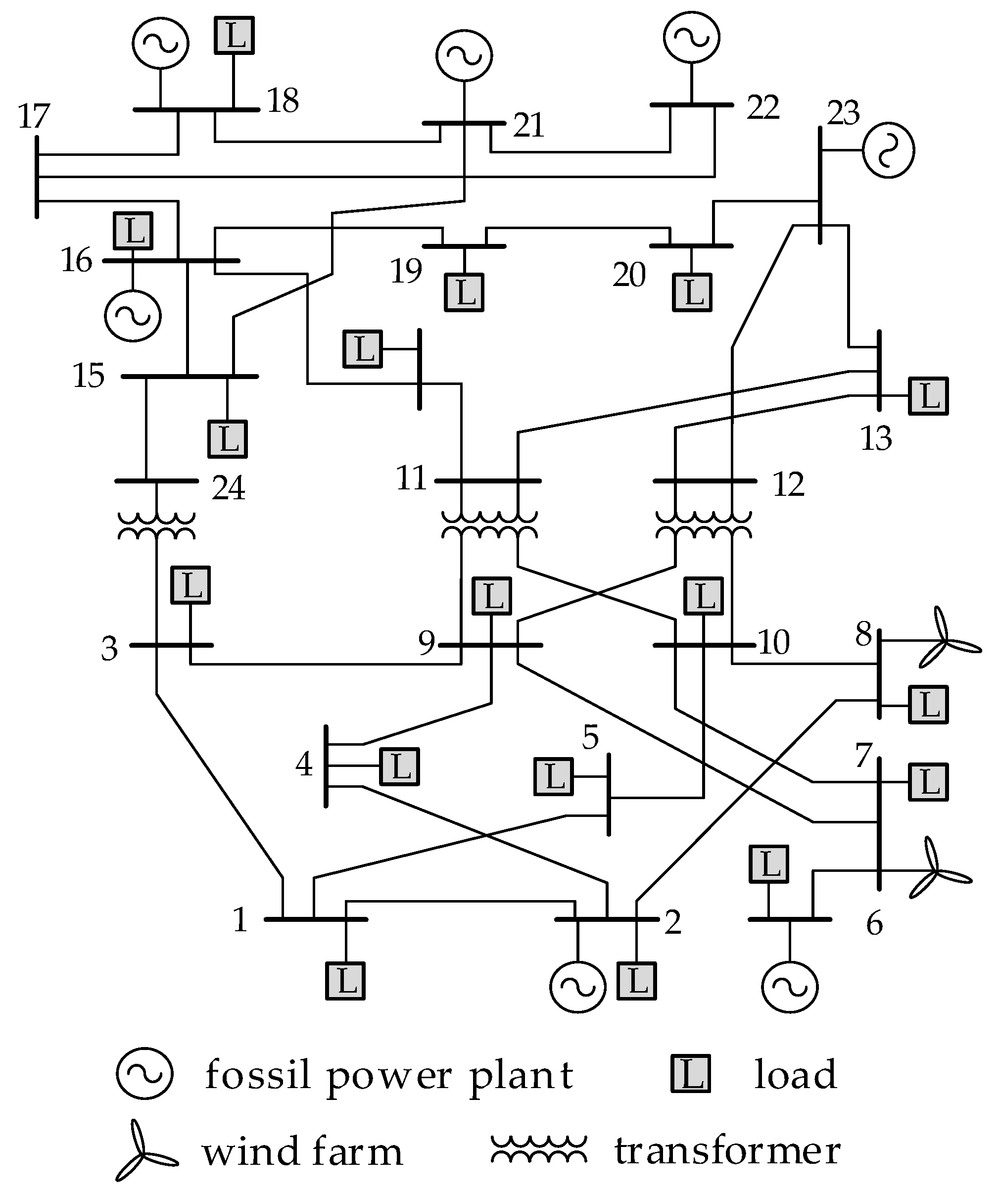
This paper uses a modified IEEE 24-node power system [25] for example analysis, which is shown in Figure 2. To verify the effectiveness of the algorithm, two wind farms are added to node 7 and 8, respectively. Supposing the wind speeds of node 7 and 8 obey normal distribution, the expectations of which are 8 m/s and 9 m/s and variances are 2 m/s and 2.2 m/s. The correlation coefficient of wind speed in node 7 and 8 is 0.99. Generally, the higher correlation coefficient of wind speed in different wind farms is, the variation trend would be more similar in these wind farms, which is to say that if the wind speed in node 7 is huge, then the wind speed in node 8 would be huge also. Therefore, if we choose the correlation coefficient of wind speed in node 7 and 8 as 0.99, which is a strong correlation relationship, then the voltage fluctuation of the power system is the most serious under this circumstance, as the system voltage average beyond limits would be more likely to occur. According to the wind speed joint distribution of nodes 7 and 8, 8000 wind speed samples are generated randomly in each wind farm. The power factor of the wind turbine is 0.98, the rated, cut-in and cut-out wind speed of the wind turbine is 15 m/s, 3 m/s and 25 m/s, respectively. Considering the rated, cut-in and cut-out wind speeds, the active and reactive power of the wind turbine can be calculated using Equations (1) and (2) according to wind speed. In reality, the uncertainty of the load is much less than that of wind speed, so we did not take the uncertainty of the load into consideration, and regard them as determined values.

5.1.2. Effectiveness Verification of the Proposed Method

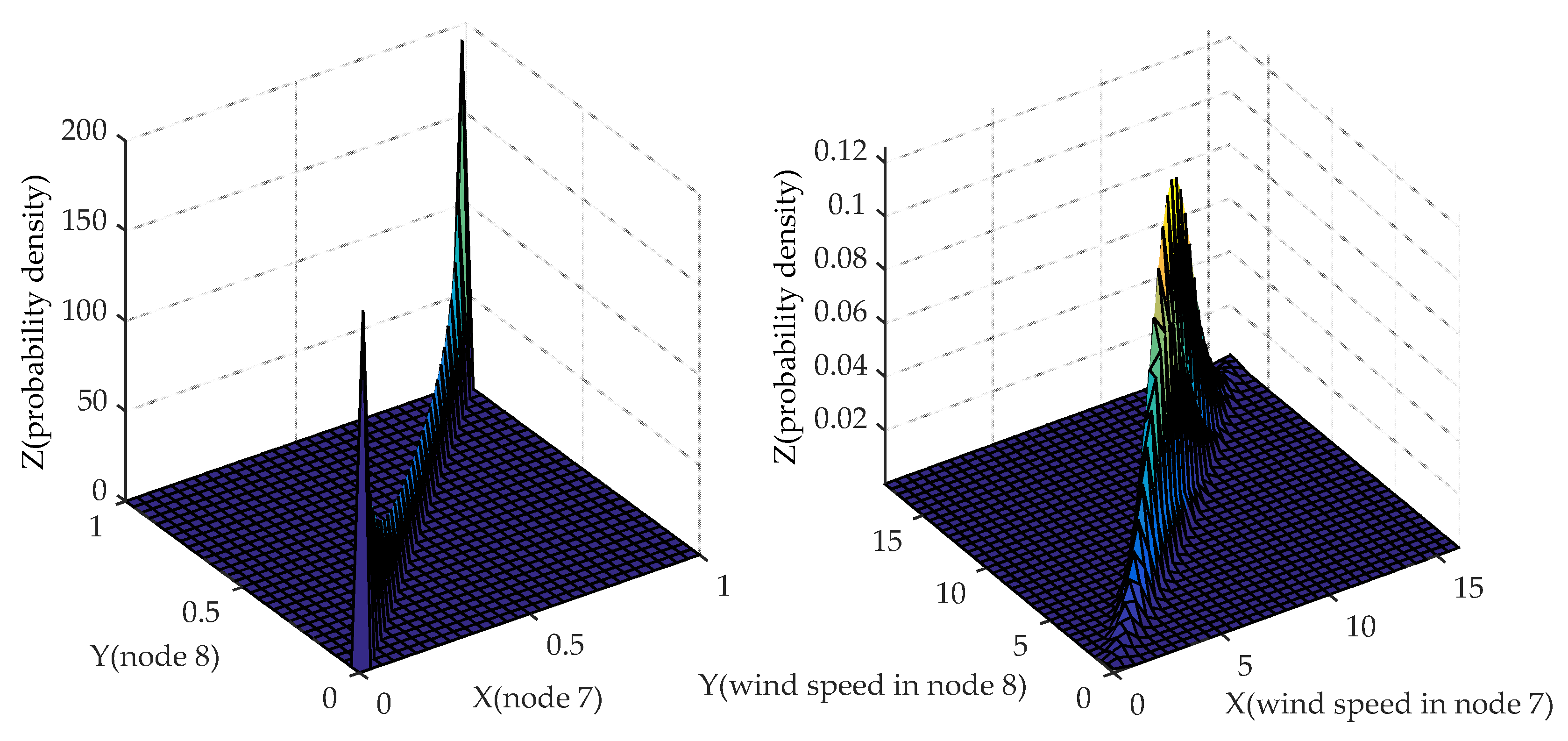
According to the 8000 generated wind speeds in Section 5.1.1, non-parametric kernel density estimation is used to obtain the probability density function of these wind speed samples, and their joint probability density function is shown in Figure 3. In this figure, the x-z and y-z planes denote the probability density function of wind speed in node 7, respectively. Apparently, the probability density function of wind speed in nodes 7 and 8 obey normal distribution because the sample number is huge, which verifies the effectiveness of using non-parametric kernel density estimation to obtain the probability density function of wind speed. In this case, we suppose that the wind speeds in node 7 and 8 obey the normal distribution in Section 5.1.1. Therefore, we select the normal copula function to establish their wind speed joint distribution model; the copula function and the joint probability density function solved through this copula are shown in Figure 4.

In order to verify the validity of joint probability density function in Figure 4, we design a method that calculates the similarity of joint probability density function between Figure 3 and Figure 4. Extract R x-axis and y-axis coordinates randomly in Figure 3 and Figure 4, and let their z-axis coordinates are $z_{ij}$ and ${\widehat{z}}_{ij}$, where i = 1, 2,…, R, j = 1, 2,…, R. Calculate the error using the formula in Equation (25), the smaller error is, the more similar joint probability density function between Figure 3 and Figure 4 is. Let R = 500, 1000, 1500, 2000, 2500, and the average error and maximum error of probability density in Figure 3 and Figure 4 are shown in

Table 2. Average error and maximum error of probability density in Figure 3 and Figure 4.

R Value	500	1000	1500	2000	2500
Average error (%)	0.68	0.59	0.74	0.73	0.85
Maximum error (%)	0.72	0.68	0.79	0.78	0.91

. We can see the errors under different R values are small enough, which verifies that the joint probability density function in Figure 4 is basically the same as that in Figure 3, and this illustrates that vine-copula could effectively construct a joint probability density of multi-dimensional random variables.

$$error={\displaystyle \sum _{i=1}^R{\displaystyle \sum _{j=1}^R\left|\frac{z_{ij}-{\widehat{z}}_{ij}}{{\widehat{z}}_{ij}}\right|}}$$

(25)

Monte Carlo sampling is used in the copula-based joint probability density function to generate 10,000 wind speed samples, and the Rosenblatt transform is used to convert the correlated wind speed samples to independent wind speed samples. On this basis, we calculate node voltage using the probabilistic load flow based on the semi-invariant method (shorthand as proposed method), and the node voltage results are shown in Figure 5. In order to verify the effectiveness of this copula and the semi-invariant based probabilistic load flow calculation in this paper, we use the Monte Carlo method to sample wind speed data in Section 5.1.1 for 10,000 times (simplified Monte Carlo method), and uses these wind speed samples to calculate power load for 10,000 times (detailed Monte Carlo method). The average error and maximum error of the proposed method and Monte Carlo method are shown in

Table 3. Average error and maximum error of simplified Monte Carlo method to detailed one.

Type	Average Error		Maximum Error
	Expectation (%)	Standard Deviation (%)	Expectation (%)	Standard Deviation (%)
Voltage amplitude	0.09	0.73	0.25	1.56
Phase angle	0.07	0.15	0.32	2.44
Active power	0.11	0.94	0.45	3.21
Reactive power	0.09	0.67	0.43	1.89

. From this Table, the calculation results of the proposed and the Monte Carlo method are basically consistent, and this illustrates that the proposed method is effective in the statistical characteristics of the output variables.

In order to verify the accuracy of the proposed method in the probability distribution characteristics of the output variables further. Taking the voltage amplitude of node 3 and node 4, the active power of branches 21-15 and 3-1, and the reactive power of branch 19-16 and 23-20 as examples, this paper calculates their distribution function using the proposed method and Monte Carlo method. The distribution functions are shown in Figure 6. From this figure, the distribution curve of these two methods are close to each other. Through verification, the distribution function of output variables in other nodes or branches using these two methods are very similar, and the maximum relative error is 2.14%, which illustrates that the proposed method could accurately obtain probability distributions, and further proves that the proposed method has higher precision.

In order to verify the novelty of the study compared with other studies, the traditional three point estimate method taking no account of wind speed correlation in [26] (traditional three point estimate method), and the three point estimate method considering wind speed correlation in [19] (improved three point estimate method) are used to sample wind speed. Then, the expectation and standard deviation of voltage amplitude and phase angle with Monte Carlo method are compared. Together with the proposed method, the average error of these three methods and the Monte Carlo method are shown in

Table 4. Average error comparison of three methods.

Method	Statistic	Voltage Amplitude	Phase Angle
Traditional three-point estimate method	Expectation	1.58	2.43
	Standard deviation	5.67	7.44
Improved three-point estimate method	Expectation	0.18	0.32
	Standard deviation	1.15	2.61
Proposed method	Expectation	0.09	0.07
	Standard deviation	0.73	0.15

. In this table, the error of the traditional three point estimate method is the largest among the three method. The reason lies in that this method take no account of wind speed correlation, which has a significant influence on the calculation results. The improved three point estimate method takes wind speed correlation into consideration, but the error is still larger than the proposed method in this paper. The method only uses the correlation coefficient as the description index of the correlation of wind speeds. In the actual situation, the correlation between wind speeds is complex and variable. Therefore, it is difficult to fully describe the relationship between these wind speeds. In fact, the linear correlation coefficient, Spearman correlation coefficient [27,28] etc. cannot fully describe the correlation between random variables; copula-based joint probability distribution is the best description.

5.2. Case Study of East Inner Mongolia Power System

5.2.1. Case Illustration and Wind Speed Data

The East Inner Mongolia region includes Chifeng region (region A), Tongliao region (region B), Hulunbeier region (region C) and Xing’an League region (region D). The East Inner Mongolia Power Grid has formed a network with 500 kV grid as the backbone network frame, 220 kV grid to achieve full coverage of the county, 110 (66) kV grid in chain ring or radiation form. By the end of 2018, the East Inner Mongolia Power Grid has 670 substations of 66 kV and above, and the transformer capacity is 65.09 million kVA and the total length of line is 37,819 km [25]. The wind speed is taken from the measured data of region A to region D. The power factor, rated wind speed, cut-in wind speed and cut-out wind speed of the wind turbine are the same as those in Section 4.1. Supposing the wind speed base value is 15 m/s, and standard the wind speed of region A to region D. Divide the standardized wind speed 0–1 to 20 intervals, and the length of each interval is 0.05, calculate the frequency and probability density the wind speed in region A to region D in each interval, which is shown as the blue bar chart in Figure 7. On this basis, non-parametric kernel density estimation is used to obtain the probability density function of wind speed in region A to region D, which is shown as the red line in Figure 7.

5.2.2. Wind Speed Joint Distribution Model of Region A to Region D

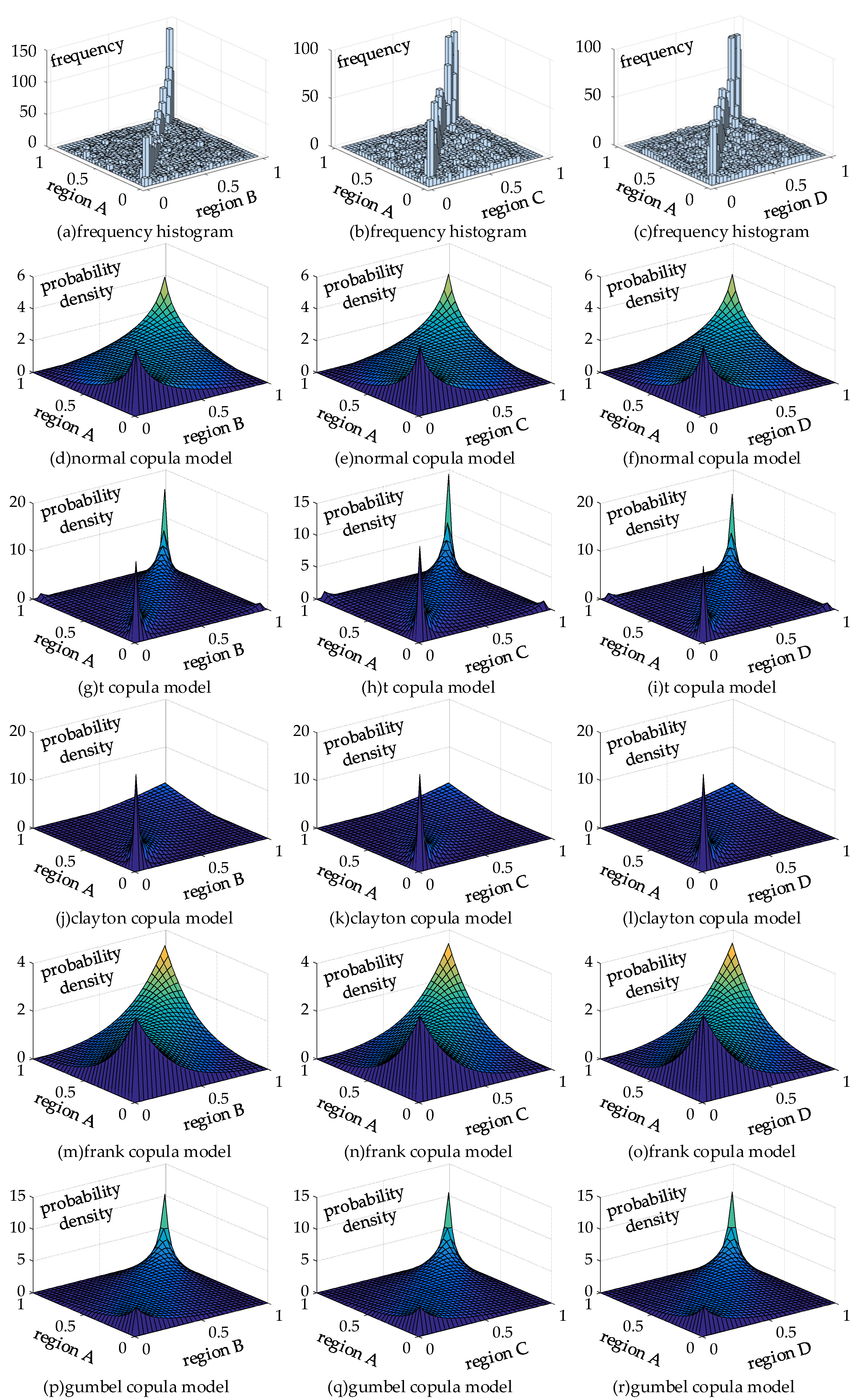
This paper uses C-vine to decompose joint distribution, and region A is regarded as the root node. The maximum likelihood estimation method is used in non-parametric kernel density estimation based probability density function of the two regions to obtain the correlation coefficient. The correlation coefficient of different copulas is shown in

Table 5. Correlation coefficient of different copulas.

Copula Type	Region A and B		Region A and C		Region A and D
Normal copula	1.00	0.38	1.00	0.40	1.00	0.39
	0.38	1.00	0.40	1.00	0.39	1.00
t copula	1.00	0.49	1.00	0.47	1.00	0.47
	0.49	1.00	0.47	1.00	0.47	1.00
Clayton copula	0.48		0.49		0.50
Frank copula	0.31		0.31		0.32
Gumbel copula	0.42		0.43		0.43

. On this basis, the probability density function of different copula types are shown in Figure 8.

In order to select the optimal copula function, this paper compares the Euclidean distance of empirical copula function and the evaluated copula function (including normal copula, t copula, gumbel copula, clayton copula and frank copula). The calculation results are shown in

Table 6. Euclidean distance of empirical copula function and the evaluated copula function.

Copula Type	Normal	t	Gumbel	Clayton	Frank
Region A and B	2.511	2.006	1.572	5.899	2.916
Region A and C	2.489	1.717	1.500	6.251	2.920
Region A and D	2.679	1.862	1.616	6.526	3.104

. From this table, we can see which Euclidean distance of the empirical copula function and gumbel copula in two different regions is smallest, so we select the gumbel copula as the optimal copula function.

5.2.3. Voltage State Assessment of East Inner Mongolia Power System

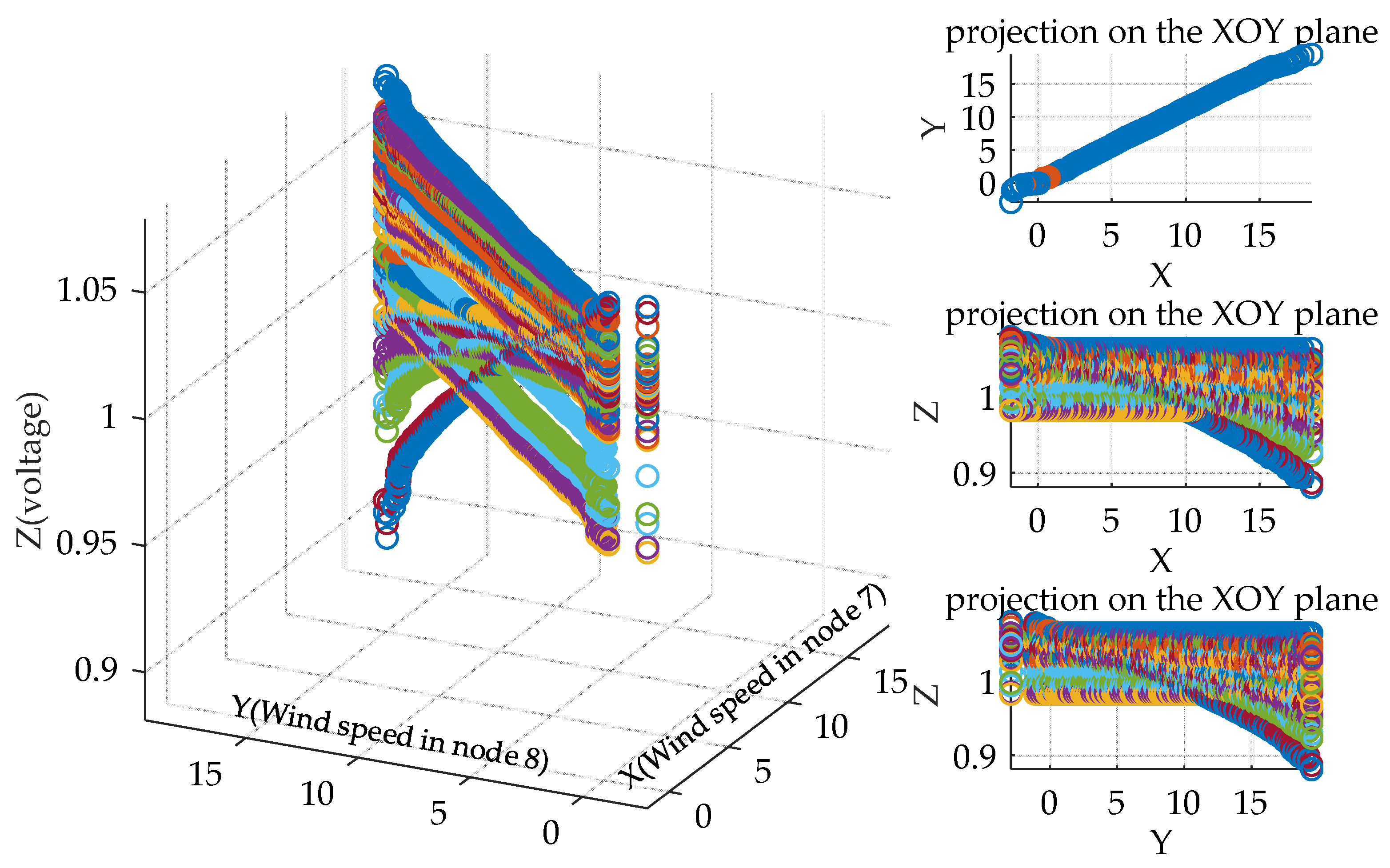
In this Section, a voltage state assessment of the East Inner Mongolia power system is evaluated. The number of wind farms in the power system is 32. Monte Carlo sampling is used for 3000 times to generate correlation wind speed samples according to the vine copula function, and the correlated wind speed samples are converted to independent wind speed samples using the Rosenblatt transform. On this basis, power flow is calculated using probabilistic load flow. The voltage amplitude results are shown in Figure 9. In this figure, we could see there exists voltage beyond limits circumstance when large-scale wind power integrated in the power system. Through verification, voltages beyond limit occur when the wind speed is huge, especially at the nodes at which wind power accessed rises more obviously as the wind speed increases; except for the nodes that wind power accessed, the nodes with load accessed are subject to voltage beyond limit circumstance as the wind speed increases, this is because the voltage adjustment ability of these nodes are weak. With the change of wind speed, the power flow value and direction are easily to change, and the voltage of these load nodes varies according to load regulation effect. The voltage of the nodes without wind power accessed, but with large capacity thermal power units, do not rise obviously or remain constant, the reason lies in that large capacity thermal power units bear the adjusting role in the power system; with a change of wind power or load, these node must adjust their output so as to meet the power supply and demand balance, so the voltage adjusting ability is ascendant in this node, and the probability of voltage beyond limits in these nodes is small.

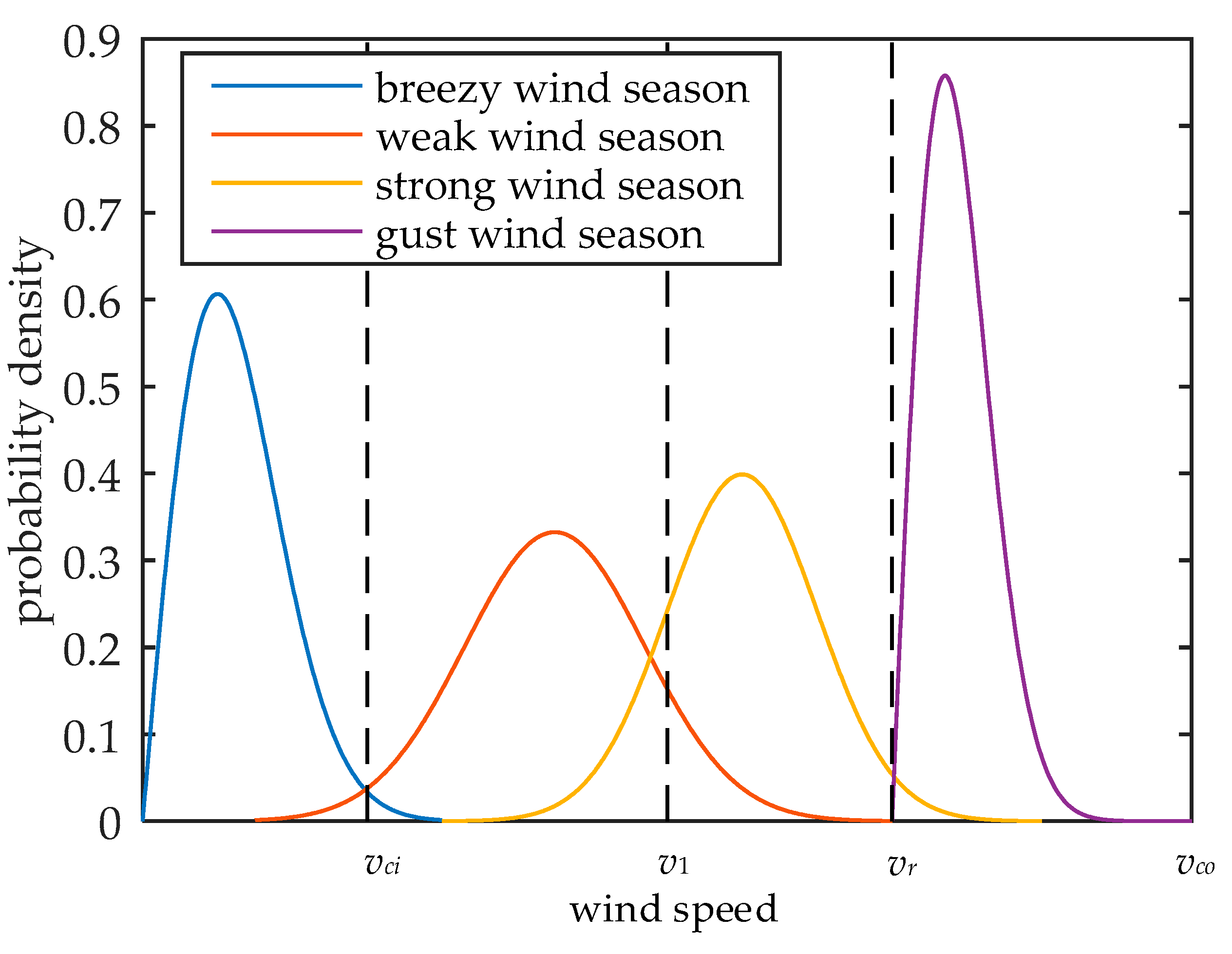
In order to evaluate the voltage state comprehensively and accurately, the power flow of wind speed distribution in different wind seasons is calculated. The wind speed distribution in different wind seasons generally includes breezy wind season, weak wind season, strong wind season and gusty wind season. Among them, gusty wind season and breezy wind season cover the windiest circumstances and constitute the weakest situation with respect to wind speed as the system will run in an extreme state. Weak wind and strong wind seasons constitute the most common situations at which the wind speed occurs, so the voltage average beyond limits problem must be studied in these two wind seasons. Therefore, this paper focuses solely on these specific wind seasons. The definition of these four wind seasons are shown in

Table 7. Definition of different wind seasons.

Wind Season	Definition
Breezy wind season	Average wind speed is below the cut-in wind speed of the turbine
Weak wind season	Average wind speed is between the cut-in wind speed and middle wind speed (between cut-in and rated wind speed) of the turbine
Strong wind season	Average wind speed is between the middle wind speed and cut-out wind speed of the turbine
Gust wind season	Average wind speed is beyond the cut-out wind speed of the turbine

.

Now, non-parametric kernel density estimation is applied to fit the wind speed distribution of these four wind seasons using wind speed samples. The Gaussian kernel function is selected as the kernel function, and the expression is shown in Equation (26), where X_i is the wind speed samples. If the window width of the Gaussian kernel function is 1, then the non-parametric kernel density estimation of the wind speed in different wind seasons can be expressed as Equation (27). Using Equations (26) and (27) to calculate the probability density function, region A is shown in Figure 10.

$$K(\cdot )=\frac{1}{\sqrt{2\pi }}\exp [-\frac{{(x-X_i)}^2}{2}]$$

(26)

$${\widehat{f}}_w(v)=\frac{1}{N}{\displaystyle \sum _{i=1}^N\frac{1}{\sqrt{2\pi }}\exp [-\frac{{(x-X_i)}^2}{2}]}$$

(27)

In order to obtain the typical system voltage beyond limits probability without reference to the randomness of wind speed, we calculate the wind speed expectation of these four wind seasons, and calculate the system voltage beyond limits probability, which is shown in

Table 8. System voltage average beyond limits probability results.

Wind Season	Breezy	Weak	Strong	Gust
System voltage beyond limits probability	0.62%	3.79%	12.73%	13.97%

. From this table, the system voltage average beyond limits probability rises with wind speed, especially in the gusty wind season. The reason lies in the increase of wind speed, when active power increases according to Equation (1). At the same time, the constant power factor control is applied to the wind turbine in this paper according to Equation (2). Therefore, the reactive power would increase with the increase of active power, and the voltage, especially the nodes with wind power accessed, would occur in the form of a voltage beyond limits circumstance.

Using the same method to obtain a wind speed joint distribution model of region A to region D, and the probabilistic load flow is calculated. On this basis, supposing system voltage beyond limits is 1.1. The system voltage average beyond limits probability is calculated, which is shown in

Table 9. System voltage average beyond limits probability results.

Wind Season	Breezy	Weak	Strong	Gust
System voltage average beyond limits probability	0.84%	4.65%	12.55%	13.63%

. From this table, system voltage average beyond limits probability rises with wind speed increases, especially in gust wind season, the system voltage average beyond limits probability reaches 13.63%. This result is the same as that we analyze in Figure 9, and this further indicates that the increase in wind speed would bring a voltage average beyond limits.

In order to calculate the node voltage exponential entropy in this power system, suppose L in Equation (23) is 30. Considering the number of the nodes is too huge, we select some node to display their node voltage exponential entropy, including the nodes containing wind power, the nodes containing thermal power and nodes only containing load. The results are shown in

Table 10. Node voltage exponential entropy results.

Node Type	Node Number	Breezy	Weak	Strong	Gust
Nodes containing wind power	1	1.98	2.41	2.04	1.82
	2	1.93	2.44	1.99	1.81
	3	2.02	2.43	2.03	1.77
Nodes containing thermal power	1	1.04	1.06	1.02	1.02
	2	1.04	1.07	1.03	1.04
	3	1.05	1.06	1.03	1.02
Nodes only containing load	1	1.27	1.62	1.53	1.39
	2	1.22	1.65	1.48	1.34
	3	1.28	1.58	1.56	1.35

. From this table, the voltage exponential entropy of different nodes is smallest in the breezy wind season, and largest in the weak wind season, which does not demonstrate sustained growth with an increase in wind speed, the reason being that the wind speed in the weak wind season is from v_ci to v₁, which is the widest range. Therefore, the voltage uncertainty in weak wind season is maximum. Besides, the voltage exponential entropy of nodes containing wind power is largest in different wind seasons, and nodes containing thermal power is smallest, nodes only containing load is between them. The reason lies in that the voltage regulation capability of wind turbines is poor, and the fluctuation of wind speed makes the voltage of this node fluctuate greatly. However, the voltage regulation capability of thermal power turbines is excellent, which could keep the voltage of this node constant.

6. Conclusions

This paper presents a vine-copula based voltage state assessment method with large-scale wind power integration. A wind speed joint distribution model of multiple regions based on vine-copula is established first, and a probabilistic load flow based on the semi-invariant method and wind speed independent transformation based on the Rosenblatt transformation are described. On this basis, a voltage state assessment index is established, and a voltage state assessment procedure is proposed. Based on the Matrix Laboratory, the case study of IEEE 24 power system and the east Inner Mongolia power system for voltage state assessment with large-scale wind power integration are provided.

(1)

This paper selected the vine-copula function to describe joint probability density of wind speeds with correlation and randomness, and the result is basically the same as that of an actual joint probability density function, and the error is under 1%, which could illustrate vine-copula’s effectiveness to construct a joint probability density of multi-dimensional random variables.

(2)

The node voltage calculation method using probabilistic load flow based on the semi-invariant method and the Monte Carlo method are basically consistent, where the expectation average error is under 0.2% and the standard deviation average error is under 1%, and this could illustrate that the proposed method is effective in the statistical characteristics of the output variables.

(3)

This paper firstly selected the vine-copula function and probabilistic load flow to assess the voltage state, and the precision of the voltage distribution function is very high compared with the traditional and improved three point estimate methods, which further proves that the proposed method has higher precision.

References

1. Adnan, R.M.; Liang, Z.; Yuan, X.; Kisi, O.; Akhlaq, M.; Li, B. Comparison of LSSVR, M5RT, NF-GP, and NF-SC Models for Predictions of Hourly Wind Speed and Wind Power Based on Cross-Validation. Energies 2019, 12, 329. [Google Scholar] [CrossRef]
2. He, P.; Arefifar, S.A.; Li, C.; Wen, F.; Ji, Y.; Tao, Y. Enhancing Oscillation Damping in an Interconnected Power System with Integrated Wind Farms Using Unified Power Flow Controller. Energies 2019, 12, 322. [Google Scholar] [CrossRef]
3. Bokde, N.; Feijóo, A.; Villanueva, D.; Kulat, K. A Review on Hybrid Empirical Mode Decomposition Models for Wind Speed and Wind Power Prediction. Energies 2019, 12, 254. [Google Scholar] [CrossRef]
4. Shen, X.; Zhou, C.; Fu, X. Study of Time and Meteorological Characteristics of Wind Speed Correlation in Flat Terrains Based on Operation Data. Energies 2018, 11, 219. [Google Scholar] [CrossRef]
5. Li, Y.; Zhou, M.; Wang, D.; Huang, Y.; Han, Z. Universal Generating Function Based Probabilistic Production Simulation Approach Considering Wind Speed Correlation. Energies 2017, 10, 1786. [Google Scholar] [CrossRef]
6. Xiong, Q.; Chen, W.; Zhang, X. Scenario Probabilistic Load Flow Calculation Considering Wind Farms Correlation. Power Syst. Technol. 2015, 39, 2154–2159. [Google Scholar]
7. Wei, Y.; Zhang, S. Copula Theory and its Ap-plications in Financial Analysis; Tsinghua University Press: Beijing, China, 2008. [Google Scholar]
8. Xie, Z.; Ji, T.; Li, M. Quasi-Monte Carlo Based Probabilistic Optimal Power Flow Considering the Correlation of Wind Speeds Using Copula Function. IEEE Trans. Power Syst. 2017, 33, 2239–2247. [Google Scholar] [CrossRef]
9. Widen, J.; Shepero, M.; Munkhammar, J. Probabilistic Load Flow for Power Grids with High PV Penetrations Using Copula-Based Modeling of Spatially Correlated Solar Irradiance. IEEE J. Photovoltaics 2017, 7, 1740–1745. [Google Scholar] [CrossRef]
10. Ning, Z.; Kang, C.; Liu, J. Mid-short-term risk assessment of power systems considering impact of external environment. J. Mod. Power Syst. Clean Energy 2013, 1, 118–126. [Google Scholar] [Green Version]
11. Aas, K.; Czado, C.; Frigessi, A.; Bakken, H. Pair-copula constructions of multiple dependence. Insurance Math. Econ. 2013, 44, 182–198. [Google Scholar] [CrossRef]
12. Yang, H.; Zou, B. A Three-point Estimate Method for Solving Probabilistic Power Flow Problems with Correlated Random Variables. Autom. Electr. Power Syst. 2012, 36, 51–56. [Google Scholar]
13. Zou, B.; Xiao, Q. Solving Probabilistic Optimal Power Flow Problem Using Quasi Monte Carlo Method and Ninth-Order Polynomial Normal Transformation. IEEE Trans. Power Syst. 2013, 29, 300–306. [Google Scholar] [CrossRef]
14. Cai, F.; Shi, D.; Chen, J. Probabilistic load flow considering correlation between input random variables based on Copula theory. Power Syst. Prot. Control 2013, 20, 13–19. [Google Scholar]
15. Wu, W.; Wang, K.; Han, B.; Li, G. Pair Copula Based Three-point Estimate Method for Probabilistic Load Flow Calculation. Trans. China Electrotech. Soc. 2015, 30, 121–128. [Google Scholar]
16. Hamada, M. Simple and efficient method for steady-state voltage stability assessment of radial distribution systems. Electr. Power Syst. Res. 2010, 80, 152–160. [Google Scholar] [CrossRef]
17. Lee, C.; Tsai, S.; Wu, Y. A new approach to the assessment of steady-state voltage stability margins using the curve. Int. J. Electr. Power Energy Syst. 2010, 32, 1091–1098. [Google Scholar] [CrossRef]
18. Toma, R.; Gavrilas, M. Voltage stability assessment for wind farms integration in electricity grids with and without consideration of voltage dependent loads, In Proceedings of International Conference & Exposition on Electrical & Power Engineering, Iasi, Romania, 20–22 October 2016.
19. Sun, G.; Chen, S.; Wei, Z. Probabilistic Optimal Power Flow of Combined Natural Gas and Electric System Considering Correlation. Autom. Electr. Power Syst. 2015, 21, 11–17. [Google Scholar]
20. Seyit, A.; Akdağ, A. A new method to estimate Weibull parameters for wind energy applications. Energy Convers. Manage. 2009, 50, 1761–1766. [Google Scholar]
21. Bedford, T.; Cooke, R. Probability Density Decompo-sition for Conditionally Dependent Random Variables Modeled by Vines. Ann. Math. Artif. Intell. 2001, 32, 245–268. [Google Scholar] [CrossRef]
22. Xu, J.; Hong, M.; Sun, Y. Dynamic scenario generation based on empirical Copula function for outputs of multiple wind farms and its application in unit commitment. Electr. Power Autom. Equip. 2017, 37, 81–89. [Google Scholar]
23. Zhang, J. Probabilistic Assessment of Static Security and Voltage Stability of Power Systems; Tianjin University: Tianjin, China, 2007. [Google Scholar]
24. Rosenblatt, M. Remarks on a Multivariate Transformation. Ann. Math. Stat. 1952, 23, 470–472. [Google Scholar] [CrossRef]
25. State Grid Mengdong Power Company Introduction. Available online: http://www.md.sgcc.com.cn/html/main/col23/2019-01/29/20190129161027185162737_1.html (accessed on 29 January 2019).
26. Pan, W.; Liu, W.; Yang, Y. Point Estimate Method for Probabilistically Optimal Power Flow Computation. In Proceedings of the 21st Conference on Software Engineering Education and Training, Charleston, SC, USA, 14–17 April; 2008; Volume 28, pp. 28–33. [Google Scholar]
27. Liu, D.; Cho, S.Y.; Sun, D.M.; Qiu, Z.D. A Spearman correlation coefficient ranking for matching-score fusion on speaker recognition. In Proceedings of the TENCON 2010–2010 IEEE Region 10 Conference, Fukuoka, Japan, 21–24 November 2010. [Google Scholar]
28. Fong, C.C.M.; De Kee, D.; Kaloni, P.N. Advanced Mathematics for Engineering and Science; World Scientific Publishing Company: London, UK, 2003. [Google Scholar]
Figure 1. The structure of C-vine.
Energies 12 02019 g001
Figure 2. A modified IEEE 24-node power system.
Energies 12 02019 g002
Figure 3. Joint probability density function of wind speed in node 7 and 8.
Energies 12 02019 g003
Figure 4. Normal copula function and the joint probability density function solved through it.
Energies 12 02019 g004
Figure 5. Node voltage results.
Energies 12 02019 g005
Figure 6. Distribution function of output variables.
Energies 12 02019 g006
Figure 7. Wind speed distribution of region A to region D.
Energies 12 02019 g007
Figure 8. Probability density function of different copula types.
Energies 12 02019 g008
Figure 9. Voltage amplitude calculation results.
Energies 12 02019 g009
Figure 10. Probability density function of region A in different wind seasons.
Energies 12 02019 g010