Complex Network Analysis of Photovoltaic Plant Operations and Failure Modes

Abstract

This paper presents a novel data-driven approach, based on sensor network analysis in Photovoltaic (PV) power plants, to unveil hidden precursors in failure modes. The method is based on the analysis of signals from PV plant monitoring, and advocates the use of graph modeling techniques to reconstruct and investigate the connectivity among PV field sensors, as is customary for Complex Network Analysis (CNA) approaches. Five month operation data are used in the present study. The results showed that the proposed methodology is able to discover specific hidden dynamics, also referred to as emerging properties in a Complexity Science perspective, which are not visible in the observation of individual sensor signal but are closely linked to the relationships occurring at the system level. The application of exploratory data analysis techniques on those properties demonstrated, for the specific plant under scrutiny, potential for early fault detection.

1. Introduction

The cumulative global photovoltaic (PV) capacity has been growing exponentially around the world over recent years. In the decade 2005–2015, the solar PV generation capacity in the EU has increased from 1.9 GW to 95.4 GW [1]. Notwithstanding this, the Europe PV market’s conditions are still substantially dependent on regional energy policies and public subsidies for renewable energies. As per the Italian market, in June 2013 the Italian public company GSE (Gestore dei Servizi Energetici) officially announced the discontinuation of the last Feed-in-Tariff incentive after its cap of 6700 million euro was reached [2]. The end of such subsidies has led to new attention being focused on PV plant performance management, lifetime and availability, with a view to reduce operating and maintenance costs [3].

Faults in PV plant components (i.e., modules, converters, connection lines), in addition to downtime correlated penalties, could result in an acceleration of system aging and as a consequence in a reduction of power plant reliability [4]. Typically, faults severity depends on various factors. These factors include the time to detect, time to repair or substitute, COE, and occurrence over time, and all of these factors can have a significant impact on profitability [5]. For these reasons, over the last decade Fault Detection and Diagnosis (FDD) in PV systems has been established as a critical field of research [6]. To mention but a few areas, research has addressed key topics like real-time monitoring, partial shading effects analysis, estimation of natural degradation rate over time and residual life for solar panels [7]. In the FDD arena, a number of studies have proposed data-driven fault detection algorithms based on statistical processing of performance parameters (e.g., power loss factor analysis studies, I-V output characteristics [8,9,10,11]) or an exponentially weighted moving average control chart [12]. In addition, model-based techniques, implementing dynamic fault trees [13] or combining PV system performance simulation (voltage ratio, performance ratio, &c) and Fuzzy and neuro-Fuzzy logic classification systems [14,15], have also been studied as methods to detect fault occurrence [16]. The open literature already offers several review papers on this field, illustrating the state-of-the-art and opportunities [4,17,18,19].

With the advent of Internet of Things, technologies for smart monitoring have found widespread applications, including in PV systems, thereby enabling decision-making processes [20]. However, monitoring systems typically employ several distributed sensors and the collection of raw data opening the field to a number of specific challenges is still unresolved, which is in part due to the different communication standards, heterogeneous structure and the huge volume of data [21,22]. As reported in a number of big data studies [23,24], traditional data analysis in statistics, management and visualization fails with sensor network data streams. High-dimensionality and heterogeneity encourage data mining and artificial intelligence solutions, such as feature extraction, classification, clustering and sampling [25,26,27,28,29,30]. Furthermore, multi-sensor data fusion techniques have been introduced to provide a robust description of an environment or process of interest by combining observations from a number of different sources [31].

In this context, complex network science emerged as an active field, cross-fertilized by natural, social and computer science, exploiting the general idea that artificial systems like biological ones (metabolic network, worldwide web, distribution network, etc.) are complex systems, composed of a large number of interacting parts (components or entities) with an articulated self-organization. The complexity of the systems, then, resides in interaction and loops among its entities [32]. Looking for example at industrial systems, constitutive elements are governed by well-defined physical laws and are included in a pre-determined process scheme. However, surrounding environments and business laws (determining the operations) influence this by-definition deterministic structure. Moving to the component level, multi-physics processes are nonlinear, as is the component matching. In a general view, these systems can evolve surfacing complex structures characterized by diversity, as well as multiple interactions within and between layers. These characteristics can make industrial systems a complex engineering system [33,34].

In this paper CNA has been used to model the sensor network of a 1 MW PV field, advocating a complex system engineering point of view [35,36]. A data fusion criterion has been developed processing the signals from the sensor equipment with a view to detect fault precursors. The sensors include PV field AC and DC electrical parameters, temperature, and solar irradiance measurements.

The paper, first, illustrates the methodology for data processing with a consideration of connectivity analysis to create the digital twin of the sensor network in the form of a functional graph. The result of these analyses is a correlation matrix that defines the graph structure in terms of the weight of the edges connecting the nodes (element/sensor signal) at a given instant from all the pairs of pre-processed sensor time series. By applying the data processing within a fixed time window, sliding over the monitoring interval, the result is a fully-connected weighted dynamic graph. Then, dynamic graph analysis is used to explore the sensor network in order to unveil hidden correlations among signal time series. The results are discussed by using exploratory data analysis to combine the most significant topological graph metrics in the identification of operational patterns of the PV plant.

2. Methodology

The field sensors are modeled using graph theory as a complex network, where the nodes are represented by the signals from sensors and the edge are evaluated with non-linear statistical correlation functions applied to the time series pairs. Specifically, the data flow is structured according to the following steps:

• data collection and pre-processing,
• connectivity analysis and graph modeling,
• pattern recognition.

At the initial stage (a), heterogeneous data acquired by the sensors are synchronized and cleaned by removing outliers. Then for stage (b), a fully-connected graph is created in which each monitored variable represents a node and all the nodes are connected to each other with directed edges. The output of this phase is a complete weighted graph model (also called functional graph) of the sensor network. After, some typical complex network measurements are applied to extrapolate synthetic properties from the functional graphs. Finally (c), these measurements were used as input for exploratory network analysis, with the aim of grouping the data as a function of multiple topological graph metrics.

The implementation of the proposed methodology has been done using Python version 3.5 [37]. In particular, a Python code has been created using Scikit-learn and NetworkX packages, respectively [38,39].

2.1. Complex Network Analysis

The CNA has its origins in graph theory and is used to describe the properties of complex systems through the mathematical study of networks. The key ingredient in the CNA is the study of the correlation among uni-variate signals recorded from different sources, as is customary for biological network analysis. For this purpose, the mutual information (MI) has been widely used [40,41,42].

In this paper we propose a novel approach based on the study of correlations between signals of m heterogeneous sensors within a fixed window of n samples. In particular, given two signals y_n,i and y_n,j, taken from the i-th and j-th component of the feature matrix Y_n,m, where (n) is spanning over time steps, the mutual information MI quantifies the level of uncertainty in y_n,i removed by the conditional knowledge of y_n,j. This measure essentially tells us how much extra information one gets from one signal by knowing the outcomes of the other one [43,44,45]. Once for each sample, a correlation matrix is obtained computing the MI in the m-dimensional feature space, while sliding the window from the beginning of the data set up to the entire monitoring interval. As a consequence, the evolution of correlation matrix is represented in the form of a functional graph consisting of a set of m nodes associated by k weighted edges representing the connecting force between the pairs of nodes.

The result of this phase is therefore a dynamic graph that contains all the information about the evolution of spatial and temporal relationships between all the entities monitored and allows the definition of parameters quantifying the characteristics of the systems [46].

In the context of CNA, the network measurements represent the most used tools for the extrapolation of synthetic information through the analysis of network topology. These measurements can be evaluated over the entire network (e.g., Shortest Path length, Diameter, Global Efficiency, Modularity, &c) or they can locally refer to nodes (e.g., Centrality Measures). This type of metric has been applied in several social networking studies to address the problem of identifying and ranking those people who exert an unequal amount of influence on the decision-making of others (also called influencers or opinion leaders) and to study the diffusion information within the network [47,48,49].

In the present approach, both the network measurements relating to the whole network (global scale) and those specific to individual nodes (local scale) were considered. Specifically, the study uses Shortest Path Length [50], Diameter and Radius of the graph [51], among the different global-scale measurements, Eccentricity and Weighted Degree Centrality of the nodes [39,52,53,54], among the local-scale measurements.

2.2. Exploratory Data Analysis

Promoted by Tukey [55], exploratory data analysis (EDA) represents a powerful tool to maximize insight into the underlying structure of a complex dataset. It facilitates the understanding of the distribution of samples and simplifies the data analysis, pointing out to special observations (outliers), clusters of similar observations, groups of related variables, and crossed relationships between specific observations and variables [56,57]. All this information in turn, can be very informative for further data modeling and it is of paramount importance to improve data knowledge. For these purposes, it encompasses a wide range of statistics and graphical tools (e.g., histogram, box plot, Pareto chart, principal component analysis, etc.) which have been commonly used for decades in various research fields such as archeology, biology, anthropology, medicine, chemometrics, &c [58,59,60].

In this paper, EDA is used to investigate the results of the complex network analysis and compare them with the sensor signals Y_n,m. In particular, the 3D scatterplot has been used for visual pattern recognition. This tool is based on a features representation in a multivariable space, allowing us to identify the dependencies between different network measurements in order to discriminate specific operational PV plant clusters.

3. Case Study

The data were collected from a PV plant with a power of 1 MWp. The solar field is connected to two inverters, each with three conversion blocks. Both inverters are grid-tied, feeding a medium voltage power distribution network. They are equipped with fully independent monitoring systems and incorporate a solar power controller to regulate the Maximum Power Point Tracking (MPPT).

Measurements were recorded every 5 min and included AC and DC electrical parameters, AC power output, ambient temperature and solar irradiance. The monitoring system is shown in Figure 1. In particular, solar radiation on the plane of the modules and ambient temperature have been measured by a pyranometer and a PT-100 RTD sensor respectively, both installed on a sensor box near the panels. Both inverters are equipped with resistive potential divider voltage sensors for DC and AC parameters measurement for each conversion block. Shunt resistors have been used to measure 12 string currents as a representative sample of the plant.

The measurements were collected in the period from May 20th to September 15th 2017. The 47 monitored variables which define the m-dimensional feature matrix Y_n,m are listed in

Table 1. Monitored PV plant variables.

Yn,1–16	Variable	Yn,17–47	Variable
1	DC Total Output Power [kW]	17	DC Voltage Inv. 1—block C [V]
2	AC Total Active Output Power [kW]	18,19,20	AC Voltage-phase 1, 2, 3 Inv. 1—block C [V]
3	Total PV Plant Energy Produced [kWh]	21	Active Output Power Inv. 2—block A [kW]
4	Ambient Air Temperature [°C]	22	DC Voltage Inv. 2—block A [V]
5	Solar Irradiance [W/m2]	23,24,25	AC Voltage-phase 1, 2, 3 Inv. 2—block A [V]
6	Active Output Power Inv. 1—block A [kW]	26	Active Output Power Inv. 2—block B [kW]
7	DC Voltage Inv. 1—block A [V]	27	DC Voltage Inv. 2—block B [V]
8,9,10	AC Voltage-phase 1, 2, 3 Inv. 1—block A [V]	28,29,30	AC Voltage-phase 1,2,3 Inv. 2—block B [V]
11	Active Output Power Inv. 1—block B [kW]	31	Active Output Power Inv. 2—block C [kW]
12	DC Voltage Inv. 1—block B [V]	32	DC Voltage Inv. 2—block C [V]
13,14,15	AC Voltage-phase 1, 2, 3 Inv. 1—block B [V]	33,34,35	AC Voltage-phase 1, 2, 3 Inv. 2—block C [V]
16	Active Output Power Inv. 1—block C [kW]	36–47	String currents [A]

.

Table 2. Main characteristics of the different sensors involved.

Sensor	Type	Measurement Range	Temperature Range
Solar radiation sensor	Pyranometer	0 to 4000 W/m2	−20 to + 50 °C
Temperature sensor	RTD (PT-100)	−50 to + 300 °C	−50 to + 300 °C
Current sensors	Shunt resistor	15 A	−40 to + 125 °C
Voltage sensors	Resistive potential divider	3 to 500 V (DC)	−40 to + 85 °C

provides the specification of the sensors used in the monitoring system. As far as the dataset is concerned, the 47 monitored variables Y_n,m are used for the connectivity analysis with a sliding window set to 216 data (about 18 h) per variable, along the available 5-months records.

4. Results

Figure 2 provides the evolution of the solar irradiance and the active power of the inverter 1 (block A) gathered from the measurement system during the period of investigation.

The interest on inverter 1 is motivated by the observation of the signals revealing the occurrence of a fault in the period between 31st August and 15th September. In particular, a breakdown of switching devices occurred, which caused the failure of the block A of inverter 1 inductor. In this case the internal protection of the inverter automatically reacted by turning off the block involved in the fault. It is worth noting that the protection reacts within the sampling interval.

Detailing on a three-day period at the end of August, the trends of the active power on the 3 blocks (from A to C) of the two inverters with the irradiation are shown in Figure 3 (inverter 2) and Figure 4 (inverter 1) respectively. The plots refer to 30th August (Figure 3a and Figure 4a), 31st August (Figure 3b and Figure 4b) and September 1st (Figure 3c and Figure 4c).

In Figure 3a and Figure 4a, August 30th plots reveals the typical operation of PV plant in sunny condition, where the solar irradiance reaches the peak value of about 950 W/m² at mid-day and the active powers of all the inverters blocks follow its trend.

Looking at the monitored data on 31st August (Figure 3b and Figure 4b), it is possible to infer that the PV plant operates under cloudy weather conditions with variations of solar irradiance. In particular, while the inverter 2 (Figure 3b) appears to work in standard conditions, following the solar radiation trend, inverter 1 (Figure 4b) starting from 13:30 features the collapse of active power on block A, which then extends to 1st September (see Figure 4c) and gives evidence of fault occurrence.

To give more hints on this fault event, Figure 5 compares the signals Y_n,7–8 and Y_n,36 gathered from inverter 1 block A (Figure 5a) and the corresponding CNA metrics. Specifically, Figure 5b illustrates the behavior of degree centralities of solar irradiance, DC voltage, AC voltage and string currents.

As confirmed by sensor signals (Figure 5a), at 13:30 the fault has an immediate effect on the string currents, while the voltages zeroed around 16:30. When looking at complex network topology measurements (Figure 5b), the fault occurrence correlates with the departure of the degree centrality of solar irradiance from those of voltage-current signals which remain correlated.

In order to understand the dynamic of the PV field operation, EDA is applied to raw data from the plant monitoring system as well as to the modeled sensor network topology variables. Figure 6, first, shows the results of the three-dimensional scatterplot of sensor signals as a function of time and solar irradiance, focusing on: the active power (Figure 6a), DC voltage (Figure 6b) and AC voltage (Figure 6c) of the inverter 1 block A. Notably, the plots refer to the sampling period from 20th May to 15th September. Data have been colored according to an agglomerative clustering.

Irrespective of the EDA variables, the analysis of the scatter plots in Figure 6a–c identify three patterns. Specifically:

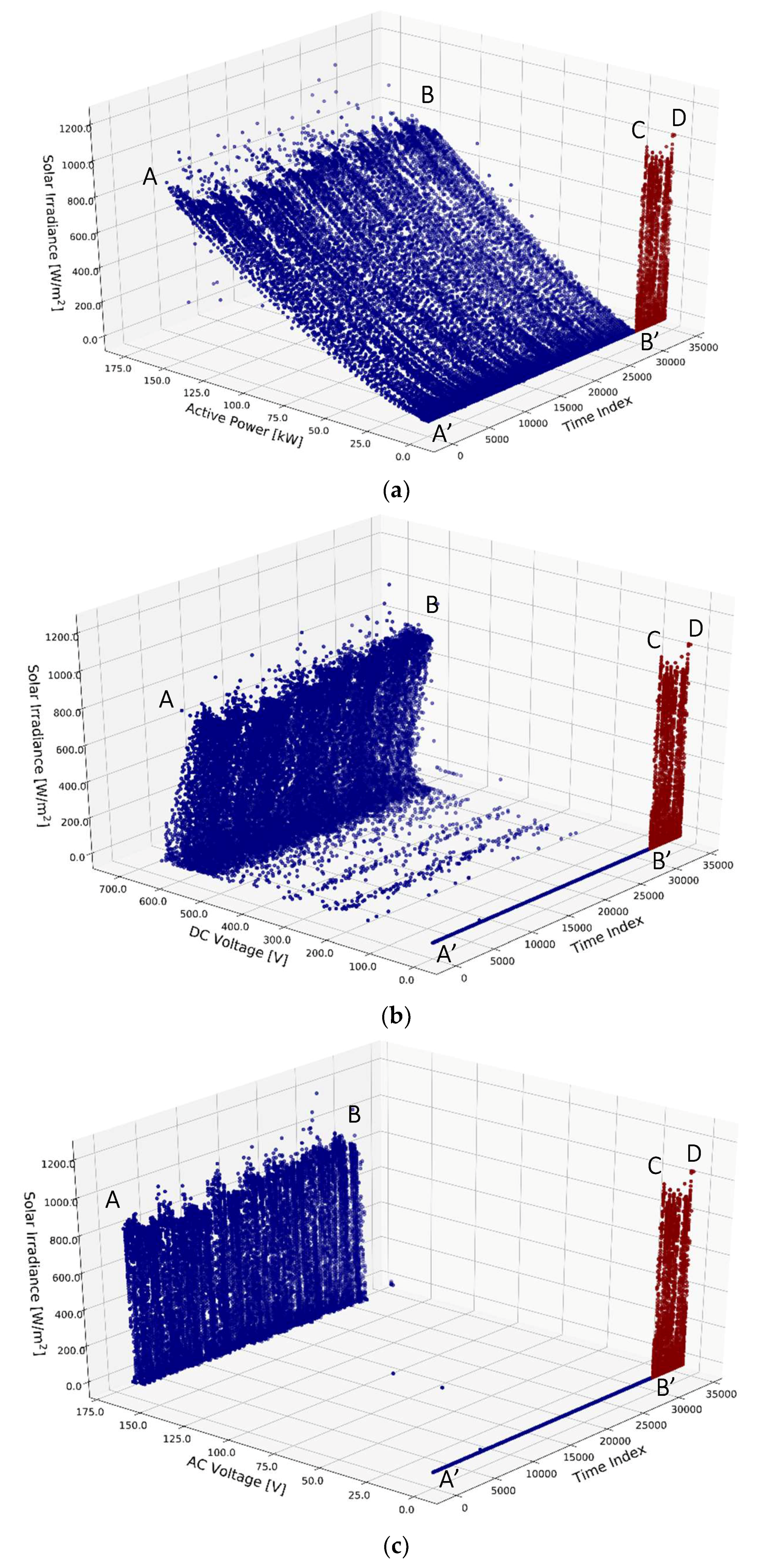
• A to B (from 00:00 of 20 May to 16:00 of 31 August), includes the sub-set of operating conditions of the inverter block with AC and DC voltages, and active power following the trend of actual solar irradiance.
• A’ to B’ (from 00:00 of 20 May to 16:00 of 31 August), includes the sub-set representative of night conditions.
• C to D (from 16:00 of 31 August to 18:00 of 15 September), then, represents the power system shutdown phase after the fault event following which AC and DC voltages, and active power zeroed.

In terms of raw data clustering, it is possible to resolve only the two behaviors which determine the operations before and after the fault event.

Figure 7 illustrates the results of EDA applied to network topology measurements. The scatter plots are created to investigate the correlation in time between a global graph measure (e.g., the graph diameter) and a local node related variable (e.g., sensor signal degree of centrality). In particular, the sensor network graph diameter is plotted against active power degree centrality (Figure 7a), AC voltage degree centrality (Figure 7b), and DC voltage degree centrality (Figure 7c).

As a first general comment, Figure 7 gives the evidence of a wealth of information emerging from the application of CNA methods. All the scatter plots demonstrate how the combination of global-local network topology measures determine the emergence of the dynamics in the PV plant operations, opening the possibility for a different performance indexing. In detail, all the plots distinguish three patterns possibly linked to the operations of the inverter block:

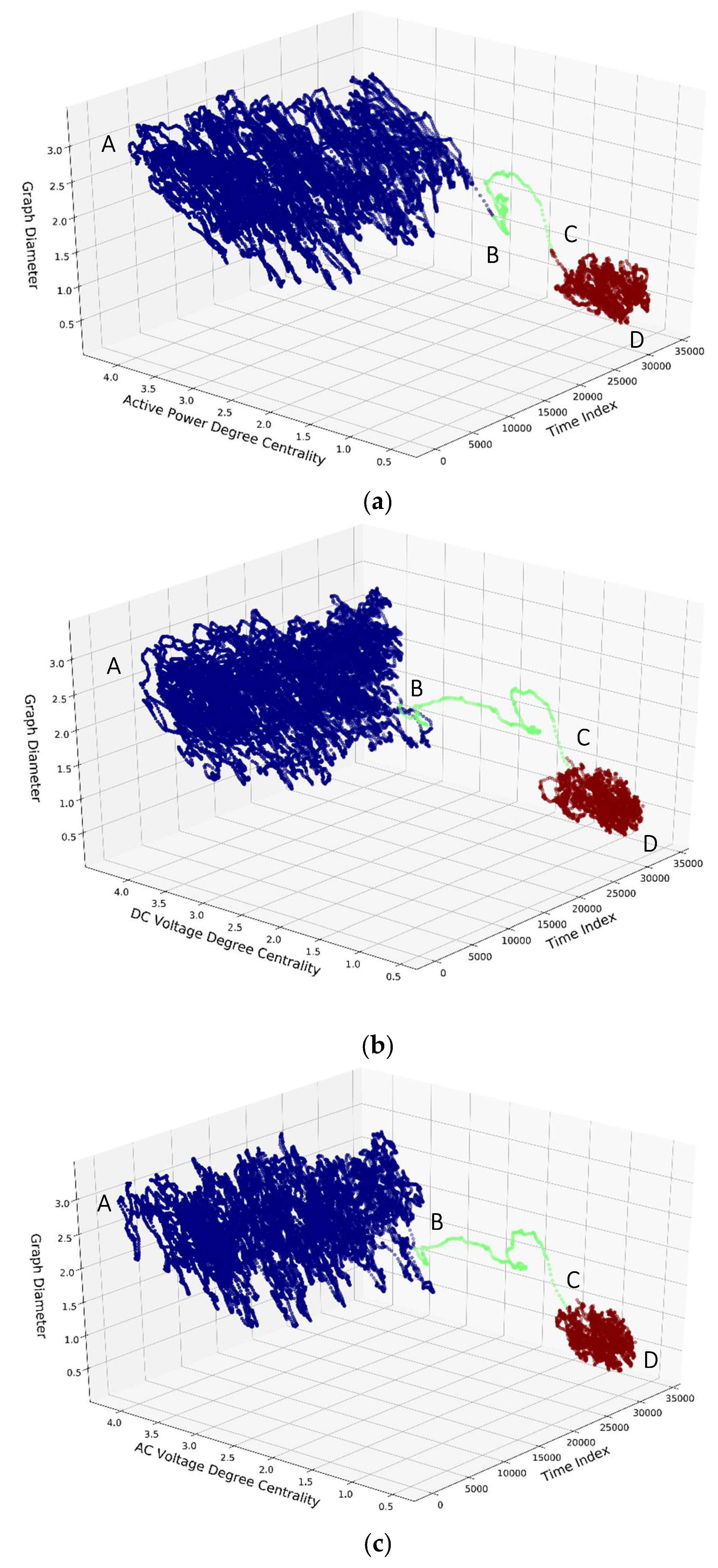
• A to B (from 00:00 of 20 May to 06:30 of 31 August), typical of the standard operation, features a degree centrality in the range 3 to 2, which is nearly proportional to the diameter of the network which experience a variation in the range 3 to 1.5.
• C to D (from 16:30 of 31 August to 18:00 of 15 September), represents the fault phase with the inverter shutdown. This cluster is characterized by low values of degree centrality (i.e., below 1) and low values of the network diameter (1.5 to 0.2).
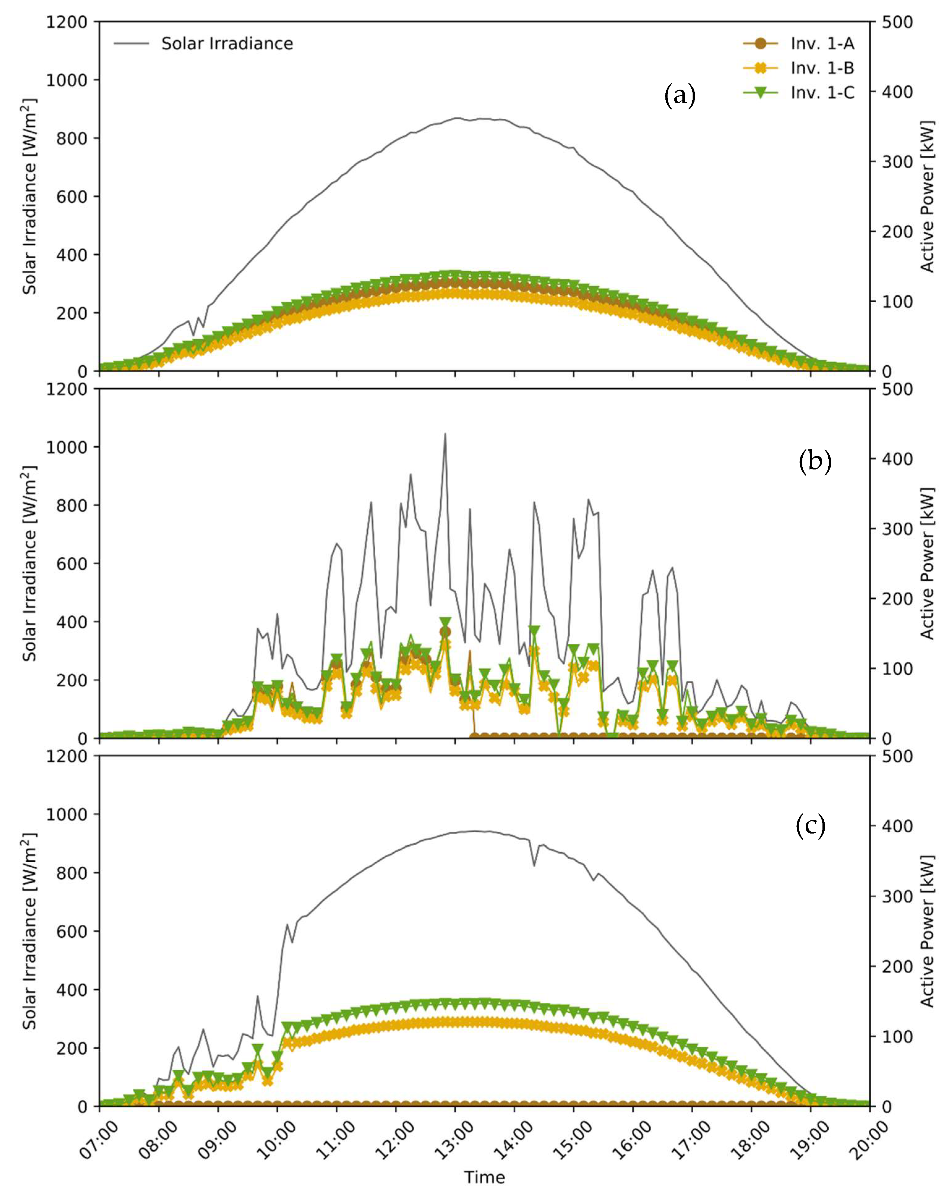
• B to C (from 06:30 to 16:30 of 31 August), finally includes the sub-set of operations that transition the inverter to fault. This cluster contains the series of points connecting the previous groups. While the network diameter ranges between 2.5 and 1.5, the degree of centralities gradually decreases from 2 to about 1 for inverter 1 block A voltages and active power. This circumstance permits us to infer that this cluster, possibly, isolates the evolution of inverter operating conditions from the precursor (6:30) to the automatic block shutdown (13:30) including also the preliminary phase of fault evolution with non-zero AC/DC voltages (16:30). As such, it demonstrates the possibility of identifying at 7 h long pre-fault event which anticipates the evolution of inverter operating conditions on 31 August.

In this case, the results of the agglomerative clustering coincide with those emerging from the scatterplots and confirm the existence of a pre-fault behavior following a nearly proportional decrease in global/local graph topology measures.

5. Conclusions

This paper proposes a sensor fusion approach based on the use of graph modeling techniques to investigate the connectivity among several key parameters of the PV plant.

The results show that the study of the properties of the graphs through the application of Complex Network Analysis techniques is able to reveal a wealth of hidden information.

As reported in Korn et al. [61] the global behavior of the system is more than the sum of its parts, so these properties can be thought of as behavior deriving from the interaction between the components that can’t be identified through their simple functional decomposition.

In particular, the visual analysis of the single topological metrics of the functional graph focused on the inverter block where the fault occurs (see Figure 4), reveals an evident variation in terms of correlation between the monitored variables, mainly associated with an anomalous deviation of the degree centrality of the solar irradiance with respect to the centrality of the key block parameters in the fault conditions.

However, by combining the multiple information deriving from the different network measurements (i.e., Degree Centrality and Network Diameter) with EDA techniques, it is possible to clearly distinguish not only the standard operation from the fault conditions, but also to isolate specific pre-fault conditions with an advance time with respect to the event of about 7 h. It is important to note that these conditions only emerge after applying CNA and are not observable with EDA techniques based on simple sensor signals. This latter type of analysis, in fact, is only able to discriminate standard operating conditions from fault conditions.

Thus, the results of this study show interesting potential in the evaluation of useful Key Performance Indicators and Control Charts based on topographic metrics of graphs for early fault detection in the PV plant.

References

1. Lacal Arantegui, R.; Jäger-Waldau, A. Photovoltaics and wind status in the European Union after the Paris Agreement. Renew. Sustain. Energy Rev. 2018, 81, 2460–2471. [Google Scholar] [CrossRef]
2. Antonelli, M.; Desideri, U. The doping effect of Italian feed-in tariffs on the PV market. Energy Policy 2014, 67, 583–594. [Google Scholar] [CrossRef]
3. Moreno-Garcia, I.M.; Palacios-Garcia, E.J.; Pallares-Lopez, V.; Santiago, I.; Gonzalez-Redondo, M.J.; Varo-Martinez, M.; Real-Calvo, R.J. Real-Time Monitoring System for a Utility-Scale Photovoltaic Power Plant. Sensors 2016, 16, 770. [Google Scholar] [CrossRef] [PubMed]
4. Mellit, A.; Tina, G.M.; Kalogirou, S.A. Fault detection and diagnosis methods for photovoltaic systems: A review. Renew. Sustain. Energy Rev. 2018, 91, 1–17. [Google Scholar] [CrossRef]
5. Richter, M.; Tjengdrawira, C.; Vedde, J.; Green, M.; Frearson, L.; Herteleer, B.; Jahn, U.; Herz, M.; Kontges, M.; Stridh, B.; et al. Technical Assumptions Used in PV Financial Models Review of Current Practices and Recommendations; Report IEA-PVPS T13-08:2017; IEA: Paris, France, 2017. [Google Scholar]
6. Houssein, A.; Heraud, N.; Souleiman, I.; Pellet, G. Monitoring and fault diagnosis of photovoltaic panels. In Proceedings of the IEEE International Energy Conference and Exhibition, Manama, Bahrain, 18–22 December 2010; pp. 389–394. [Google Scholar]
7. Spagnuolo, G.; Xiao, W.; Cecati, C. Monitoring, Diagnosis, Prognosis, and Techniques for Increasing the Lifetime/Reliability of Photovoltaic Systems. IEEE Trans. Ind. Electron. 2015, 62, 7226–7227. [Google Scholar] [CrossRef] [Green Version]
8. Muhammad, N.; Zakaria, N.Z.; Shaari, S.; Omar, A.M. Fault detection approach in photovoltaic system using Mathematical method diagnosis. J. Fundam. Appl. Sci. 2018, 10, 270–281. [Google Scholar]
9. Davarifar, M.; Rabhi, A.; Elhajjaji, A.; Dahmane, M. Real-time Model base Fault Diagnosis of Photovoltaic Panels Using Statistical Signal Processing. In Proceedings of the International Conference on Renewable Energy Research and Applications, Madrid, Spain, 20–23 October 2013; pp. 599–604. [Google Scholar]
10. Hassan Ali, M.; Rabhi, A.; Elhajjaji, A.; Tina, G.M. Real Time Fault Detection in Photovoltaic Systems. Energy Procedia 2017, 111, 914–923. [Google Scholar]
11. Chen, Y.H.; Liang, R.; Tian, Y.; Wang, F. A novel fault diagnosis method of PV based-on power loss and I-V characteristics. IOP Conf. Ser. Earth Environ. Sci. 2016, 40, 012022. [Google Scholar] [CrossRef] [Green Version]
12. Garoudja, E.; Harrou, F.; Sun, Y.; Kara, K.; Chouder, A.; Silvestre, S. Statistical fault detection in photovoltaic systems. Sol. Energy 2017, 150, 485–499. [Google Scholar] [CrossRef]
13. Chiacchio, F.; Famoso, F.; D’Urso, D.; Brusca, S.; Aizpurua, J.I.; Cedola, L. Dynamic Performance Evaluation of Photovoltaic Power Plant by Stochastic Hybrid Fault Tree Automaton Model. Energies 2018, 11, 306. [Google Scholar] [CrossRef]
14. Dhimish, M.; Holmes, V.; Mehrdadi, B.; Dales, M. Multi-layer photovoltaic fault detection algorithm. High Volt. 2017, 2, 244–252. [Google Scholar] [CrossRef]
15. Bonsignore, L.; Davarifar, M.; Rabhi, A.; Tina, G.M.; Elhajjaji, A. Neuro-Fuzzy fault detection method for photovoltaic systems. Energy Procedia 2014, 62, 431–441. [Google Scholar] [CrossRef]
16. Ventura, C.; Tina, G.M. Development of models for on-line diagnostic and energy assessment analysis of PV power plants: The study case of 1 MW Sicilian PV plant. Energy Procedia 2015, 83, 248–257. [Google Scholar] [CrossRef]
17. Abdulmawjood, K.; Refaat, S.S.; Morsi, W.G. Detection and prediction of faults in photovoltaic arrays: A review. In Proceedings of the IEEE 12th International Conference on Compatibility, Power Electronics and Power Engineering, Doha, Qatar, 10–12 April 2018; pp. 1–8. [Google Scholar]
18. Chokor, A.; El Asmar, M.; Lokanath, S.V. A Review of Photovoltaic DC Systems Prognostics and Health Management: Challenges and Opportunities. In Proceedings of the Annual Conference of the Prognostics and Health Management Society, Denver, CO, USA, 3–6 October 2016; pp. 43–54. [Google Scholar]
19. Triki-Lahiani, A.; Bennani-Ben Abdelghani, A.; Slama-Belkhodja, I. Fault detection and monitoring systems for photovoltaic installations: A review. Renew. Sustain. Energy Rev. 2018, 82, 2680–2692. [Google Scholar] [CrossRef]
20. Gubbi, J.; Buyya, R.; Marusic, S.; Palaniswami, M. Internet of Things (IoT): A vision, architectural elements, and future directions. Future Gener. Comput. Syst. 2013, 29, 1645–1660. [Google Scholar] [CrossRef] [Green Version]
21. Macaluso, I.; Galiotto, C.; Marchetti, N.; Doyle, L. A complex systems science perspective on wireless networks. J. Syst. Sci. Complex. 2016, 29, 1034–1056. [Google Scholar] [CrossRef]
22. Corsini, A.; Bonacina, F.; Feudo, S.; Marchegiani, A.; Venturini, P. Internal Combustion Engine sensor network analysis using graph modeling. Energy Procedia 2017, 126, 907–914. [Google Scholar] [CrossRef]
23. Zhou, K.; Fu, C.; Yang, S. Big data driven smart energy management: From big data to big insights. Renew. Sustain. Energy Rev. 2016, 56, 215–225. [Google Scholar] [CrossRef]
24. Yu, N.; Shah, S.; Johnson, R.; Sherick, R.; Hong, M.; Loparo, K. Big Data Analytics in Power Distribution Systems. In Proceedings of the IEEE Power & Energy Society Innovative Smart Grid Technologies Conference, Washington, DC, USA, 18–20 February 2015; pp. 1–5. [Google Scholar]
25. Daliento, S.; Chouder, A.; Guerriero, P.; Massi Pavan, A.; Mellit, A.; Moeini, R.; Tricoli, P. Monitoring, Diagnosis, and Power Forecasting for Photovoltaic Fields: A Review. Int. J. Photoenergy 2017, 2017, 1356851. [Google Scholar] [CrossRef]
26. Riley, D.; Johnson, J. Photovoltaic Prognostics and Heath Management using Learning Algorithms. In Proceedings of the 38th IEEE Photovoltaic Specialists Conference, Austin, TX, USA, 3–8 June 2012; pp. 1535–1539. [Google Scholar]
27. Chine, W.; Mellit, A.; Bouhedir, R. FPGA-Based Implementation of an Intelligent Fault Diagnosis Method for Photovoltaic Arrays. In Artificial Intelligence in Renewable Energetic Systems; Springer: Cham, Switzerland, 2018; pp. 245–252. [Google Scholar]
28. De Benedetti, M.; Leonardi, F.; Messina, F.; Santoro, C.; Vasilakos, A. Anomaly detection and predictive maintenance for photovoltaic systems. Neurocomputing 2018, 310, 59–68. [Google Scholar] [CrossRef]
29. Jiang, L.L.; Maskell, D.L. Automatic Fault Detection and Diagnosis for Photovoltaic Systems using Combined Artificial Neural Network and Analytical Based Methods. In Proceedings of the IEEE International Joint Conference on Neural Networks, Killarney, Ireland, 12–17 July 2015; pp. 1–8. [Google Scholar]
30. Mohamed, A.H.; Nassar, A.M. New Algorithm for Fault Diagnosis of Photovoltaic Energy Systems. Int. J. Comput. Appl. 2015, 114, 26–31. [Google Scholar] [CrossRef]
31. Waltz, E.; Llinas, J. Multisensor Data Fusion; Artech House: Boston, MA, USA, 1990; Volume 685. [Google Scholar]
32. Newman, M.E.J. The Structure and Function of Complex Network. Siam Rev. 2003, 45, 167–256. [Google Scholar] [CrossRef]
33. Kauffman, S.A. The Origins of Order: Self-Organization and Selection in Evolution; Oxford University Press: New York, NY, USA, 1993. [Google Scholar]
34. Asbjørnsen, O.A. Systems Engineering Principles and Practice; SKARPODD Co.: Arnold, MD, USA, 1992. [Google Scholar]
35. Pestov, I.; Verga, S. Dynamical networks as a tool for system analysis and exploration. In Proceedings of the IEEE Symposium on Computational Intelligence for Security and Defense Applications, Ottawa, ON, Canada, 8–10 July 2009; pp. 1–8. [Google Scholar]
36. Carbone, A.; Jensen, M.; Sato, A.H. Challenges in data science: A complex systems perspective. Chaos Solitons Fractals 2016, 90, 1–7. [Google Scholar] [CrossRef]
37. Python Version 3.5.6, 2018. Available online: http://www.python.org (accessed on 15 October 2018).
38. Pedregosa, F.; Varoquaux, G.; Gramfort, A.; Michel, V.; Thirion, B.; Grisel, O.; Blondel, M.; Prettenhofer, P.; Weiss, R.; Dubourg, V.; et al. Scikit-learn: Machine learning in Python. J. Mach. Learn. Res. 2011, 12, 2825–2830. [Google Scholar]
39. Hagberg, A.A.; Swart, P.J.; Schult, D.A. Exploring Network Structure, Dynamics, and Function using NetworkX. In Proceedings of the 7th Python in Science Conference, Pasadena, CA, USA, 19–24 August 2008; pp. 11–16. [Google Scholar]
40. Stögbauer, H.; Grassberger, P.; Kraskov, A. Estimating Mutual Information. Phys. Rev. E 2004, 69, 066138. [Google Scholar]
41. Kraskov, A. Synchronization and Interdependence Measures and their Applications to the Electroencephalogram of Epilepsy Patients and Clustering of Data. Ph.D. Thesis, John von Neumann Institute for Computing (NIC) Series, Jülich, Germany, 2004. [Google Scholar]
42. Mason, S.P.; Barabási, A.L.; Oltvai, Z.N.; Jeong, H. Lethality and centrality in protein networks. Nature 2001, 411, 2–41. [Google Scholar]
43. Kern, A.D.; Hahn, M.W. Comparative genomics of centrality and essentiality in three eukaryotic protein-interaction networks. Mol. Biol. Evol. 2005, 22, 803–806. [Google Scholar]
44. Wibral, M.; Lindner, M.; Pipa, G.; Vicente, R. Transfer entropy—a model-free measure of effective connectivity for the neurosciences. J. Comput. Neurosci. 2011, 30, 45–67. [Google Scholar]
45. Quiroga, R.Q.; Bhattacharya, J.; Pereda, E. Nonlinear multivariate analysis of neurophysiological signals. Prog. Neurobiol. 2005, 77, 1–37. [Google Scholar] [Green Version]
46. Guye, M.; Bettus, G.; Bartolomei, F.; Cozzone, P.J. Graph theoretical analysis of structural and functional connectivity MRI in normal and pathological brain networks. Magn. Reson. Mater. Phys. Biol. Med. 2010, 23, 409. [Google Scholar] [CrossRef]
47. Freeman, L.C. Centrality in social networks: Conceptual clarification. Soc. Netw. 1979, 1, 39–215. [Google Scholar] [CrossRef]
48. Sànchez-Hernàndez, G.; Casabayò, M.; Agell, N.; Puigbò, J.Y. Influencer detection approaches in social networks: A current state-of-the-art. Front. Artif. Intell. Appl. 2014, 269, 261–264. [Google Scholar]
49. Hacid, H.; Favre, C.; Zighed, D.A.; Guille, A. Information diffusion in online social networks: A survey. Acm Sigmod Rec. 2013, 42, 17–28. [Google Scholar]
50. Granger, C.W.J. Testing for causality: A personal viewpoint. J. Econ. Dyn. Control 1980, 2, 329–352. [Google Scholar] [CrossRef]
51. Scardoni, G.; Laudanna, C. Centralities Based Analysis of Complex Networks. New Front. Graph Theory 2012, 323–348. [Google Scholar] [CrossRef]
52. Das, K.C.; Maden, A.D.G.; Cangul, I.N.; Cevik, A.S. On Average Eccentricity of Graphs. Proc. Natl. Acad. Sci. India Sect. A Phys. Sci. 2017, 87, 23–30. [Google Scholar] [CrossRef]
53. Koschützki, D.; Schreiber, F. Centrality Analysis Methods for Biological Networks and Their Application to Gene Regulatory Networks. Gene Regul. Syst. Biol. 2008, 2, 193–201. [Google Scholar] [CrossRef]
54. Tamassia, R.; Tollis, I.G.; Di Battista, G.; Eades, P. Graph Drawing: Algorithms for the Visualization of Graphs; Prentice Hall: Upper Saddle River, NJ, USA, 1998. [Google Scholar]
55. Tukey, J.W. The Future of Data Analysis. Ann. Math. Stat. 1962, 33, 1–67. [Google Scholar] [CrossRef]
56. Yu, C.H. Exploratory data analysis in the context of data mining and resampling. Int. J. Psychol. Res. 2010, 3, 9–22. [Google Scholar] [CrossRef]
57. Seltman, H.J. Experimental Design and Analysis; Carnegie Mellon University: Pittsburgh, PA, USA, 2012. [Google Scholar]
58. Ho, T.K.; Basu, M.; Law, M.H.C. Data Complexity in Pattern Recognition; Springer Science & Business Media: Berlin, Germany, 2006. [Google Scholar]
59. Camacho, J.; Pérez-Villegas, A.; Rodríguez-Gómez, R.A.; Jiménez-Mañas, E. Multivariate Exploratory Data Analysis (MEDA) Toolbox for Matlab. Chemom. Intell. Lab. Syst. 2015, 143, 49–57. [Google Scholar] [CrossRef]
60. Komorowski, M.; Marshall, D.C.; Salciccioli, J.D.; Crutain, Y. Exploratory Data Analysis. Secondary Analysis of Electronic Health Records; Springer: Cham, Switzerland, 2016; pp. 185–203. [Google Scholar]
61. Korn, B.; Dohler, H. A System is More Than the Sum of Its Parts—Conclusion of DLR’S Enhanced Vision Project ADVISE-PRO. In Proceedings of the 25th AIAA/IEEE Digital Avionics Systems Conference, Portland, OR, USA, 15–19 October 2006; pp. 1–8. [Google Scholar]
Figure 1. Schematic block circuit diagram of the PV system with sensors and measuring points.
Energies 12 01995 g001
Figure 2. Solar irradiance and active power of the inverter 1 (block A) during the period of investigation.
Energies 12 01995 g002
Figure 3. Analysis of sensor signals of the Inverter 2 on 30st August (a), on 31th August (b) and on 1st September (c)—Solar Irradiance over the Active Power of the inverter blocks.
Energies 12 01995 g003
Figure 4. Analysis of sensor signals of the Inverter 1 on 30st August (a), on 31th August (b) and on 1st September (c)—Solar Irradiance over the Active Power of the inverter blocks.
Energies 12 01995 g004
Figure 5. Analysis of (a) sensor signals from block A of the inverter 1 compared with (b) sensor network CNA metrics on 31st August.
Energies 12 01995 g005
Figure 6. Exploratory data analysis applied to sensor signals from block A of the inverter 1. Trends of (a) active power, (b) DC voltage and (c) AC voltage (x-axis), against solar irradiance (y-axis) and time (z-axis).
Energies 12 01995 g006
Figure 7. Exploratory data analysis applied to complex network measurements from block A of the inverter 1. Trends of (a) active power, (b) DC voltage and (c) AC voltage normalized weighted degree centralities (x-axis), against network diameter (y-axis) and time (z-axis).
Energies 12 01995 g007