Spatio-Temporal Model for Evaluating Demand Response Potential of Electric Vehicles in Power-Traffic Network

Abstract

Electric vehicles (EVs) can be regarded as a kind of demand response (DR) resource. Nevertheless, the EVs travel behavior is flexible and random, in addition, their willingness to participate in the DR event is uncertain, they are expected to be managed and utilized by the EV aggregator (EVA). In this perspective, this paper presents a composite methodology that take into account the dynamic road network (DRN) information and fuzzy user participation (FUP) for obtaining spatio-temporal projections of demand response potential from electric vehicles and the electric vehicle aggregator. A dynamic traffic network model taking over the traffic time-varying information is developed by graph theory. The trip chain based on housing travel survey is set up, where Dijkstra algorithm is employed to plan the optimal route of EVs, in order to find the travel distance and travel time of each trip of EVs. To demonstrate the uncertainties of the EVs travel pattern, simulation analysis is conducted using Monte Carlo method. Subsequently, we suggest a fuzzy logic-based approach to uncertainty analysis that starts with investigating EV users’ subjective ability to participate in DR event, and we develop the FUP response mechanism which is constructed by three factors including the remaining dwell time, remaining SOC, and incentive electricity pricing. The FUP is used to calculate the real-time participation level of a single EV. Finally, we take advantage of a simulation example with a coupled 25-node road network and 54-node power distribution system to demonstrate the effectiveness of the proposed method.

1. Introduction

1.1. Motivation and Background

Persistent growth of the global economy is causing issues relating to energy supply, environmental pollution, and dependence on fossil fuels, all of which need to be addressed with a sense of urgency [1]. To better tackle these problems, many countries have been committing to support the development of electric vehicle technologies as well as provide incentives to encourage the use of EVs (e.g., battery electric vehicles (BEV) and plug-in hybrid vehicles (PHEV)) [2]. It means that more and more EVs will be connected to the grid and interact with the utility in the future. On the one hand, EVs are a flexible power load [3], they will require charging from the grid at different times and at different locations [4,5]. As a consequence, the coordination of EVs’ charging has been widely studied in the recent period [6,7]. On the other hand, it is also a kind of distributed energy storage resource. Since EVs have a lot of time to dwell in the parking lots during the day, they have great potential to participate in the power system DR service [8,9]. However, due to the flexibility and randomness of electric vehicle behavior and the uncertainty of participation in demand response [10], it is difficult to assess the potential of participation in demand response events, especially under the power-traffic hybrid network, which is important for the planning and operation of the power grid and transportation, therefore, an assessment of spatio-temporal uncertainties and user participation uncertainties in EV-DR is inevitable. It is worth noting that because different types of EVs have a different charging time, charging power, and battery capacity, we focus on BEVs in this paper.

1.2. Literature Overview

Motivated by the above reasoning, at present, many researchers have carried out EV and grid interaction related research, in particular, user-side management, EVs’ demand response. Reference [11] analyzes the users’ power transfer, reduction behavior, and the response to the demand of dispatching in the context of time-of-use electricity price and pricing strategy. In [12], an algorithm for distributed EVs’ DR to shape the daily demand profile in a day-ahead market is presented. The authors in [13] provided a collaborative evaluation of dynamic-pricing and peak power limiting-based DR strategies for home energy management (HEM). The authors in [14] make full use of the EVs’ DR capability and propose a corresponding frequency control strategy. Also, in [15], the author investigated a charging and discharging strategy for EVs that can utilize the DR capability of V2G in residential distribution networks. However, EVs’ DR capability is assumed to be activated only after the vehicles arrive home. The authors in [16] presented an intelligent energy management framework with DR capability for industrial facilities, yet the user’s willingness to participate DR program was ignored. In a recent work [17], an EV parking lot energy management system is present in consideration of the uncertainties of the arrival and departure time, and the remaining state-of-energy of EVs just before charging operation.

Valuable insights of EVs demand response works were provided in previous studies. However, it is worth mentioning that in the previously cited approaches, only the EVs’ time-varying charging/discharging characteristics were taken into account, they consider EVs as a type of fixed load or response resource, while the location of EVs is commonly disregarded. In addition, the previous studies’ take on EVs is that they can participate in DR events when EVs have objective controlled ability, ignoring the uncertainty of user participation willingness, the subjective participation degree of users is not considered in detail.

1.3. Contributions

Thus, our focus in this paper is the EV demand response potential evaluation from the perspective of spatio-temporal distribution and vehicle owner participation capability. The main contributions of this work are summarized as follows.

(1)

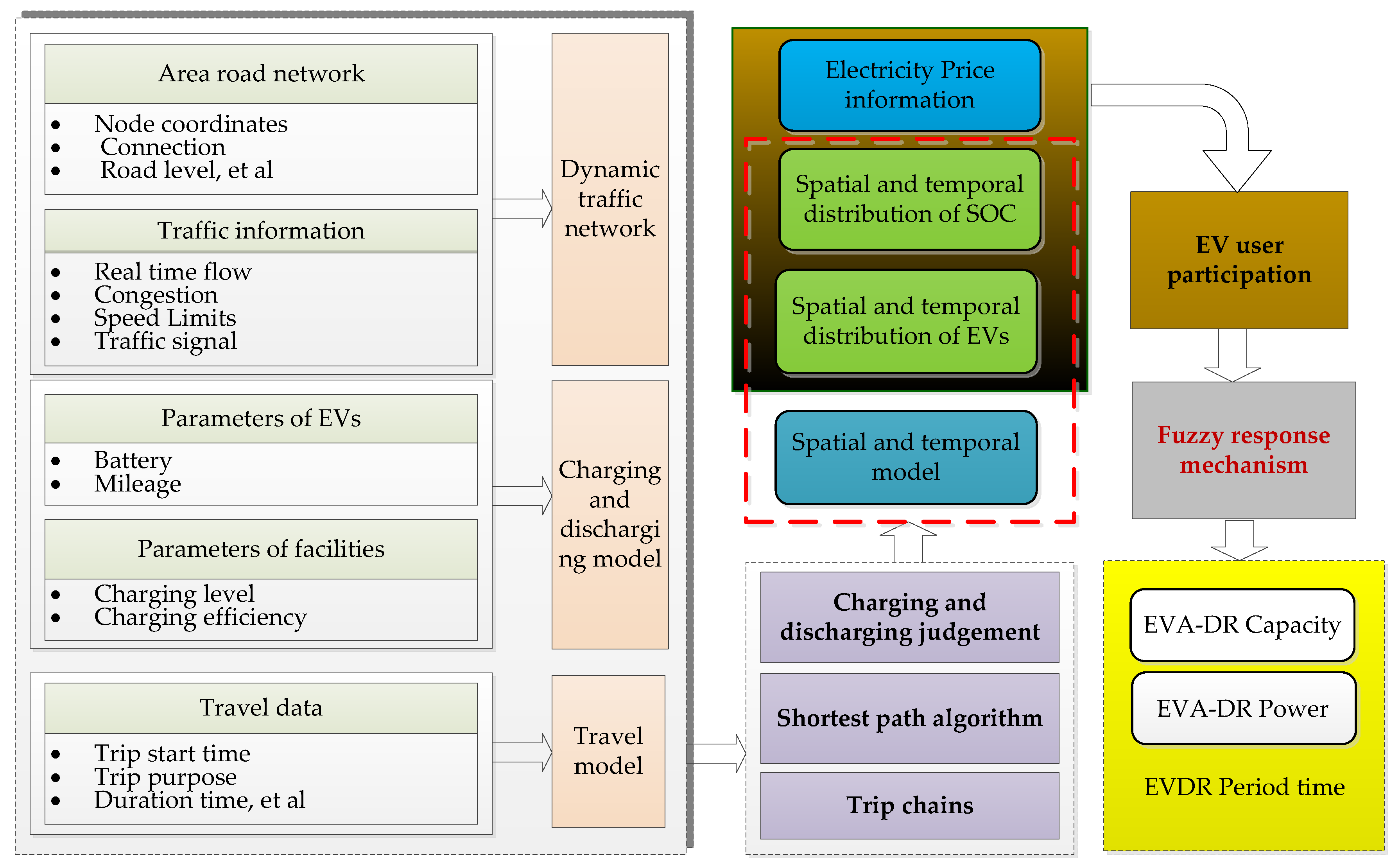
Aspects beyond the characteristics of spatial distribution of EVs and travel pattern analysis have been neglected in the existing literature, we model a dynamic traffic network considering the traffic time-varying information with randomness in travel behavior based on trip chains.

(2)

A method to analyze EVs’ objective and subjective participation in a DR event is developed.

(3)

Differently from the fixed demand response mode in the related research, we proposed a fuzzy logic-based mechanism, we modeled uncertainties that affect the estimation of demand response potential of a single EV and EVA. Three key factors—the remaining parking time, the remaining SOC, and incentive electricity pricing—are considered.

(4)

The real-time participation level of a single EV and EVA from a spatio-temporal scope in the power-traffic network are evaluated.

The remainder of this paper is organized as follows: In Section 2, we formulate the spatio-temporal model of electric vehicle travel patterns based on trip chains under dynamic road network. In Section 3, the objective participation ability as well as the subjective participation ability of EV users are considered, and the EVs DR mechanism is obtained by fuzzy algorithm. In Section 4, the case study and the results are presented, analyzed, and discussed. Conclusions are drawn in Section 5.

2. EVs Travel Model in Dynamic Traffic Network

The proposed electric vehicles aggregator demand response evaluation (EVA-DRE) method is illustrated in Figure 1. The first part of the method is EVs’ travel modeling to get the spatial and temporal distribution, which will be introduced in this section. Another part is the EV user participation modeling and response mechanism to obtain the EV-DR power and capacity.

In this section, we will provide a general method for simulating the daily travel pattern with dynamic traffic network and trip chains. First, the time-dependent dynamic road network model is established by using graph theory. Travel characteristics of EVs are then analyzed. Furthermore, the process of the travel pattern simulation is presented.

2.1. Time-Dependent Dynamic Road Network Model

During the day’s travel of a private electric vehicle, it will depart from the starting point which we assume the house, and it will pass through one or more trip destinations, including multiple trip, and the choice of each travel route will be affected by the road network and traffic conditions. Yet, the traffic conditions of the road network change over time as shown in

Table 1. Dynamic travel time of each road section.

	Time Intervals	1	2	…	k	…
Road Sections/links
1		t1(1)	t1(2)	…	t1(k)	…
2		t2(1)	t2(2)	…	t2(k)	…
…		…	…	…	…	…
r		tr(1)	tr(2)	…	tr(k)	…
…		…	…	…	…	…

. In addition, graph theory is usually adopted to describe the complicated actual road network [18]. In this work, the traffic time-varying information is considered in the road network, as in Equation (1).

$$\{\begin{array}{l}G=(V,E,W,D,T)\\ V=\{1,2,\dots ,n\}\\ E=\left\{e_{ij}\right|i,j\in V\}\\ W=\{t_r(k)|r\in E,k\in T\}\\ D=\{t_d(k)|d\in V,k\in T\}\\ T=\left\{k\right|k=1,2,\dots ,K\}\end{array}$$

(1)

where, the vertex $V$ of the graph $G$ represents the intersection of the road, and the edge $E$ of the graph represents the section between the two adjacent intersections, and the set of road weights $W$ is used for describing various road lengths, travel times, and other attributes, D is the set of the delayed time of all intersections. $t_r(k)$ is the travel time function at time slot $k$ of link r, $t_d(k)$ is the delayed time in the intersection d at time slot k; T represents the time set, and K is the total number of time intervals in a day.

2.2. Spatio-Temporal Travel Characteristics of EVs

Suppose that EV users will go to one or more destinations during a day’s travel, and the EV charging and discharging may occur in these trip destinations.

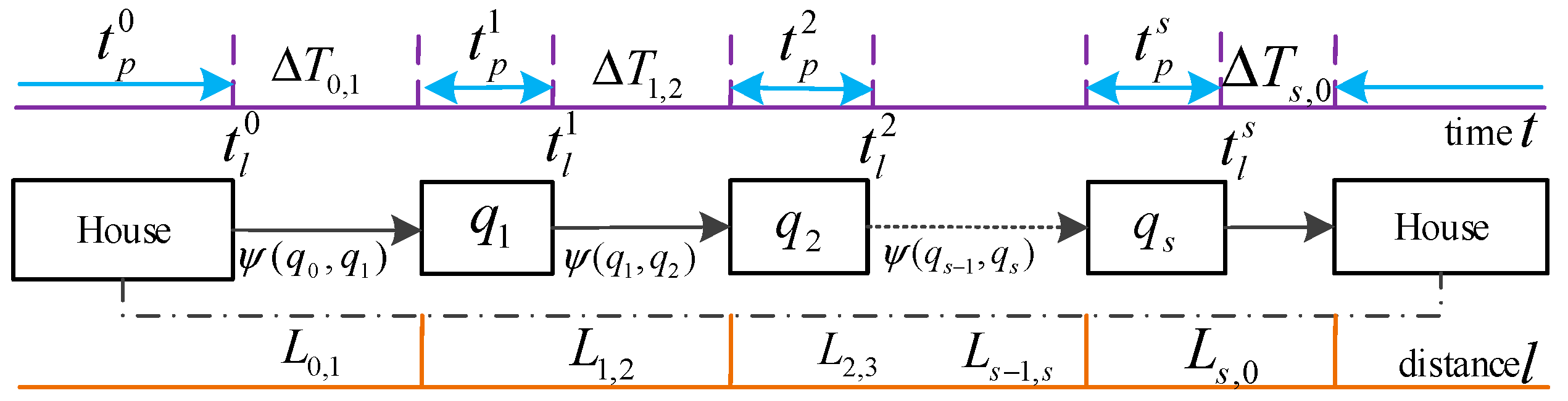
2.2.1. Trip Chains and Travel Route Planning

We use daily trip chains [19,20,21] which are created to show the whole travel routes in one day with spatial and temporal information, shown in Figure 2 and Equation (2).

$$Q=\left\{q_0(x_0,y_0),q_1(x_1,y_1),\cdots ,q_s(x_s,y_s),\cdots \right\}$$

(2)

where, $Q$ is the set for the duration trip destinations of the trip chain, $s$ is the number of the duration trip destinations, $q_0,q_1\dots q_s$ indicate all of the trip destinations, $(x_s,y_s)$ is the corresponding coordinates, $q_0$ is the first place of the trip chain which is considered to be the house in this paper.

A path among consecutive trip destinations in the trip chain is represented by $\psi (q_s,q_{s+1})$. The path set that characterizes the EV’s spatial travel process is expressed as $\Pi$ in Equation (3).

$$\Pi =\left\{\psi (q_0,q_1),\psi (q_1,q_2),\cdots ,\psi (q_s,q_{s+1}),\cdots \right\}$$

(3)

Let $t_l^i,t_p^i(i=0,1,2,\dots ,s,\dots )$ be the departure time and the parking duration time in the $i^{th}$ trip destination, respectively, and $t_p^0$ is the dwelling time in the house. In Figure 2, $L_{i,i+1}(i=0,1,2,\dots ,s-1,\dots )$ and $\Delta T_{i,i+1}$ are the travel distance and travel time between two trip destinations, respectively.

2.2.2. Departure Time of the First Trip

Here, we consider the departure time $t_l^0$ of the EVs’ first trip in a daily horizon to be randomly distributed according to probability distribution function (pdf) as

$$t_l^0~f(t_l^0)$$

(4)

2.2.3. Traveling and Traveled Time

In a completed trip, EVs will path several links and several intersections. Hence, it is necessary to draw the required time to pass each link at a certain time when calculating the travel time between two destinations. Some existing link travel time functions are discussed in [22], and the traffic time-consuming coefficient is used to calculate the travel time of the road segment under the corresponding traffic index, which is more than the time-consuming multiple in the unblocked state. The logit-based volume delay function [23] as in Equation (5) is used for depicting travel time.

$$t(s,s+1)={\displaystyle \sum _{r=1}^{n_r}{t}_r(k)}+{\displaystyle \sum _{d=1}^{m_d}{t}_d(k)}$$

(5)

where,

$$\{\begin{array}{l}{t}_r(k)=t_0·c_1·{\left[1-\frac{c_2}{1+\exp (c_3-c_4·{\theta }_r(k))}\right]}^{-1}\\ t_d(k)=t_0·p_1·\left[1+\frac{p_2}{1+\exp (p_3-p_4·{\lambda }_r(k))}\right]\\ {\theta }_r(k)=\frac{q_r(k)}{C_r},{\lambda }_r(k)=\frac{q_r(k)}{X_r}\\ t_0=\frac{l_r}{v_0},r\in E\end{array}$$

(6)

where, $t(s,s+1)$ represents the traveling time from s to s + 1; $n_r,m_d$ are the total links and the total intersections between s and s + 1, respectively; $t_0,v_0$ are the free-flow traveling time and free-flow driving speed which are related to the road grades, respectively; $l_r$ is the length of link $r$, in km; $q_r(k)$ is the real-time traffic of link $r$ at time slot k; $C_r$ and $X_r$ represent road capacity and intersection capacity of link $r$, respectively; saturation of traffic volume ${\theta }_r(k)$ and ${\lambda }_r(k)$ are used to characterize the congestion factor (traffic index), the greater the values, the more congested roads and junctions; $c_i(i=1,2,3,4)$ are the adaptive coefficients that related to road grades, $p_i(i=1,2,3,4)$ are the adaptive coefficients of the intersection related to whether there is a traffic light.

2.2.4. Arrival and Departure Time at the Destination

The arrival and departure time of every trip’s destination can be obtained by Equation (7).

$$\{\begin{array}{l}{t}_a^s=t_l^0+{\displaystyle \sum _{i=0}^{s-1}t(i,i+1)}+{\displaystyle \sum _{i=1}^{s-1}{t}_p^i}\\ t_l^s=t_a^s+t_p^s\end{array}$$

(7)

where, $t_a^s$ and $t_l^s$ are the arrival and departure time at the trip destination, $t_p^s$ is the parking time.

2.2.5. Parking Times

In this paper, it is also assumed that parking duration $t_p^s$ of the EVs in non-residential areas—i.e., office, shopping mall—follows a probability distribution $t_p^s~f(t_p^s)$. In addition, the parking duration in the residential area can be obtained by Equation (8).

$$t_p^h=\{\begin{array}{l}{t}_l^h-t_a^h,\hspace{1em}\hspace{1em}0<t_a^h<0.5K\\ t_l^h-t_a^h+K,\hspace{1em}0.5K\le t_a^h\le K\end{array}$$

(8)

where, $t_p^s$ and $t_p^h$ represent the parking time at trip destination s and in the house, respectively; $t_a^h,t_l^h$ are the arrival and departure times at the house, respectively.

2.2.6. Route Planning

When the vehicle travels from the current location (source point) to a destination (destination point), the vehicle users tend to select the route in advance, and the users will choose different road resistances according to their different preferences, such as driving distance, travel time, road quality, congestion situation, travel expenses, etc. We assume that the user considers ‘travel time’ as the important basis for route selection. Therefore, the minimum travel time, which includes road travel time and traffic light delay time, is set as the target for the shortest path planning, i.e., Dijkstra’s algorithm [24].

2.3. EV Battery SOC Estimate

When EVs arrive at a destination, when there is no demand response event, the user will decide whether to replenish the energy for their EV according to the current battery SOC and the next trip, is defined as,

$$\{\begin{array}{l}S(t_a^s)·E_m-{\displaystyle \sum _{r=1}^{n_{s,s+1}}{\omega }_r·l_r}\le {\zeta }_0·E_m\\ S(t_a^s)=S(t_a^{s-1})-({\displaystyle \sum _{r=1}^{n_{s-1,s}}{\omega }_r·l_r)/E_m}\end{array}$$

(9)

where, $S(t_a^s)$ is the SOC at arrival time of destination s; $E_m$ is the battery capacity of EV m, in kWh; ${\omega }_r$ is the energy consumption per kilometer, in kWh/km; ${\zeta }_0$ is preset by EV user; $n_{s-1,s}$ and $n_{s,s+1}$ represent the number of links between two trip destinations. Likewise, the battery state of leaving the trip destination is obtained.

$$\{\begin{array}{l}S(t_l^s)=\{\begin{array}{l}S(t_a^s),\gamma =0\\ \min \left\{S(t_a^s)+\Delta S(t_p^s),S_{set},S_{up}\right\},\gamma =1\\ \max \left\{S(t_a^s)+\Delta S(t_p^s),S_{set},S_{low}\right\},\gamma =-1\end{array}\\ \Delta S(t_p^s)=\gamma ·\delta ·\frac{P_c^s·t_p^s}{E_m}\end{array}$$

(10)

where, $S(t_l^s)$ is the SOC at the departure time; $P_c^s$ is the rated charging power; $\gamma$ is a flag sign, 0, 1, and −1 are no charging, charging and discharging, respectively; $\delta$ is the charging/discharging efficiency; $S_{set}$ is the SOC of the departure time set by EV user; $S_{up}$ and $S_{low}$ represent the upper limit considering the battery life and the minimum limit to support the next trip, respectively.

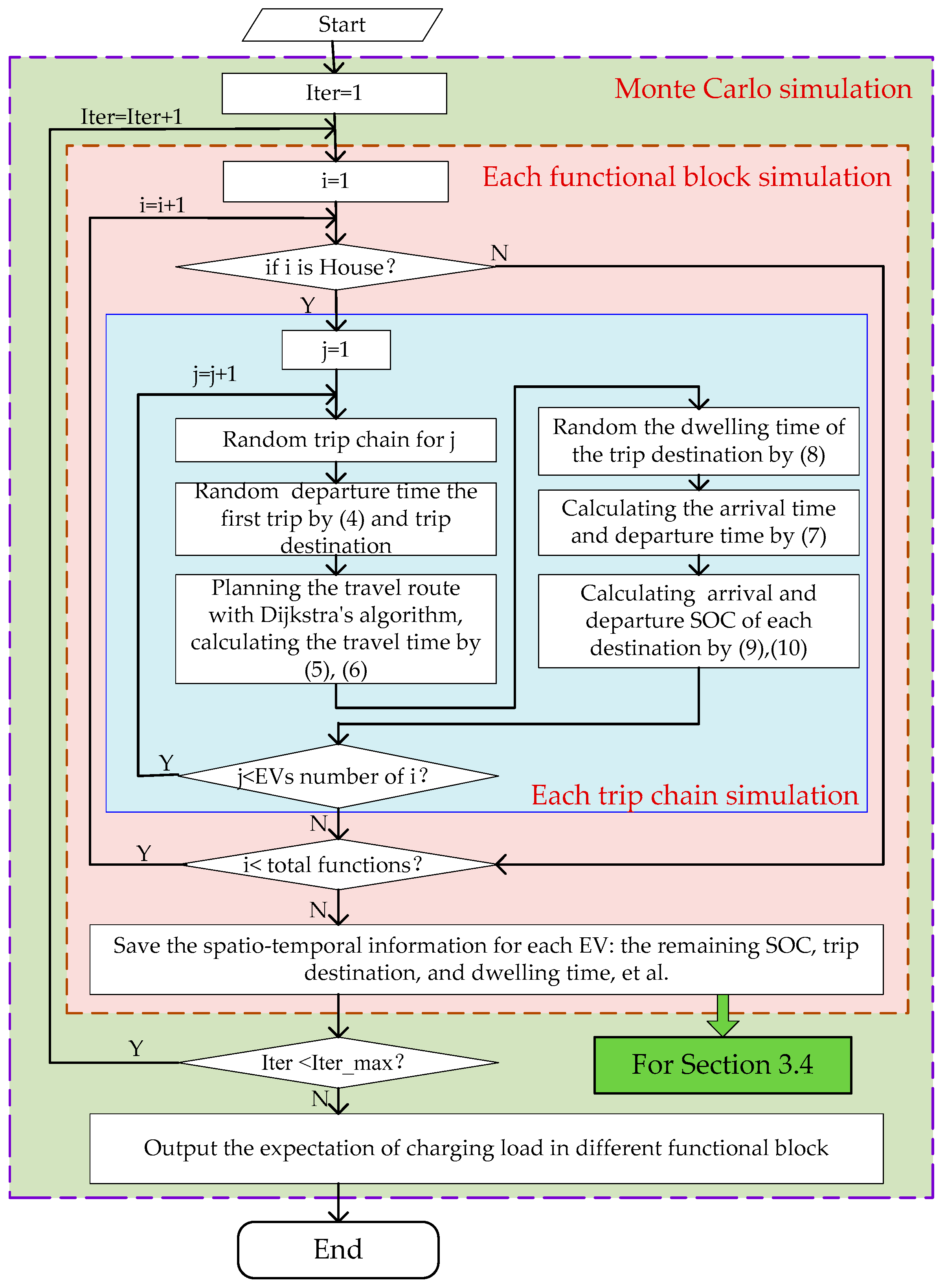
2.4. Travel Pattern Simulation

The temporal and geographical information of EVs in a travel day can be obtained by performing the following six key steps:

Step 1.

Obtain the survey results of residents from the transportation department and analyze the structure type of the vehicles’ trip chains.

Step 2.

The space movement state of the vehicle is determined according to the trip chain structure that the travel destinations of the vehicle are clear.

Step 3.

The first departure time of the vehicle is extracted by Equation (4) according to the type of travel chain Equation (2).

Step 4.

The travel path space and time between two consecutive trip destinations are determined by the path planning algorithm and Equations (3), (5), and (6).

Step 5.

Extract the dwell time of the different destinations according to Equation (8). The arrival and departure time are calculated by Equation (7).

Step 6.

The state of charge of the battery in each destination is judged and calculated by Equations (9) and (10).

Through Step 1 to Step 6, we can obtain the spatio-temporal characteristics of each EV in a travel day, including the remaining SOC, the travel destination, and its dwell time. The simulation flowchart is shown in Figure 3. Monte Carlo simulation will be carried out with EVA-DRE process which will be presented in Section 3.4.

3. Methodology for EVA-DRE

Having obtained the modeling of EVs travel pattern in the dynamic road network, including spatial and temporal information and SOC distribution, analyzing the user participation ability is of importance to evaluate the demand response potential upon each destination. A fuzzy rule response mechanism with three key factors are then considered in this section. The temporal and geographical distribution of single EV and EVA demand response capacity is obtained by Monte Carlo simulation.

3.1. User Participation of EVs DR

EV users usually exhibit complete rationality, limited rationality and satisfactory decision-making in the process of charging and discharging power consumption. When EVs arrive at a destination, it is only possible to participate in the actual DR event when they objectively have the DR capability. Otherwise, even if the EV user has a strong willingness to participate, it is unable to participate in the DR event. Here, the DR participation is divided into three categories: (1) participate in adjusting the charging time (delayed charging), (2) participate in the discharge case, (3) have no DR capability.

3.1.1. Objective Participation Ability

We introduce the objective participation ability $K_m^s(t)$ here to show the actual participation of EVs DR, which is presented as Equation (11) and illustrated in detail as

Table 2. Objective participation ability of EVs under different situation.

	Situation	Remaining SOC	Whether to Meet the Next Trip Demand	Dwelling Time	Enough Time to Replenish	Objective Participation Ability
Cases
A		Sufficient	Yes	-	-	1
B		Insufficient	No	Long	Yes	1
C		Insufficient	No	Short	No	0

.

$$\{\begin{array}{l}{K}_m^s(t)=\{\begin{array}{l}1, \mathrm{A} or \mathrm{B}\\ 0, \mathrm{C}\end{array}\\ \mathrm{A}:\Delta S\ge S_{lim}\\ \mathrm{B}:\Delta S<S_{lim} \& t_{ch}^s<\Delta T_{sur}^s\\ \mathrm{C}:\Delta S<S_{lim} \& t_{ch}^s\ge \Delta T_{sur}^s\\ \Delta S=S(t_a^s)-S(t(s,s+1))\\ t_{ch}^s=\frac{\Delta S\times E_m}{\delta \times P_c^s}\end{array}$$

(11)

where, $\Delta S$ is the current available SOC; $S(t(s,s+1))$ is the SOC consumed by the vehicle from s to s + 1; $S_{lim}$ is the minimum residual capacity level to prolong battery life; $\Delta T_{sur}^s$ indicates the remaining time of the vehicle to the next trip; $t_{ch}^s$ is the required charging time. EVs in cases of A and B have the capability of objective participation, but for C, regardless of parking time or SOC, it mismatches for its next trip driving requirement, thus, EVs in case C should charge the battery immediately. The charging power can be calculated by Equation (12).

$$\{\begin{array}{l}{P}_C^s(t)=P_c^s{\displaystyle \sum _{m=1}^{N^C(t)}\zeta (t)}\\ \zeta (t)=\{\begin{array}{l}1,t_a^s<t<t_a^s+t_{ch}^s\\ 0,\mathrm{else}\end{array}\end{array}$$

(12)

where, $P_C^s(t)$ is the total charging power of EVs in case C of time t at the destination of s; $N^C(t)$ is the number of EVs in case C at time t.

3.1.2. Subjective Participation Willingness

For different EV owners, they will make different decisions whether to participation in a DR event always based on the current state of charge, electricity price, and remaining travel time. Even the same electric vehicle owner may have different decision-making results due to random factors such as mood at the time.

We define ${\rho }_m(t)$ as subjective participation, to characterize the subjective willingness of EV users to participate in a DR event. Then, the subjective participation degree of A, B, and C in Section 3.1.1 can be described as Equation (13).

$$\{\begin{array}{l}A:0\le {\rho }_m^{del}(t)\le 1,0\le {\rho }_m^{v2g}(t)\le 1\\ B:0\le {\rho }_m^{del}(t)\le 1,0\le {\rho }_m^{v2g}(t)\le 1\\ C:{\rho }_m^{del}(t)=0,{\rho }_m^{v2g}(t)=0\end{array}$$

(13)

where ${\rho }_m^{del}(t)$ and ${\rho }_m^{v2g}(t)$ are the delayed and V2G participation degree of EV users, respectively.

Meanwhile, the subjective participation is limited by objective responsiveness, and it is to be satisfied as

$${\rho }_m(t)=f({\alpha }_m(t),{\beta }_m(t),{\gamma }_m(t)||K_m^s(t))$$

(14)

where, three essential factors ${\alpha }_m(t)$, ${\beta }_m(t)$, and ${\gamma }_m(t)$ are considered, which represent the remaining parking time, the remaining SOC, and the incentive price at the current time, respectively. It should be mentioned that, Equation (14) is an uncertainty function, thus, to focus on the uncertainty of EVs DR participation, fuzzy algorithm is used to calculate EV user demand responsiveness.

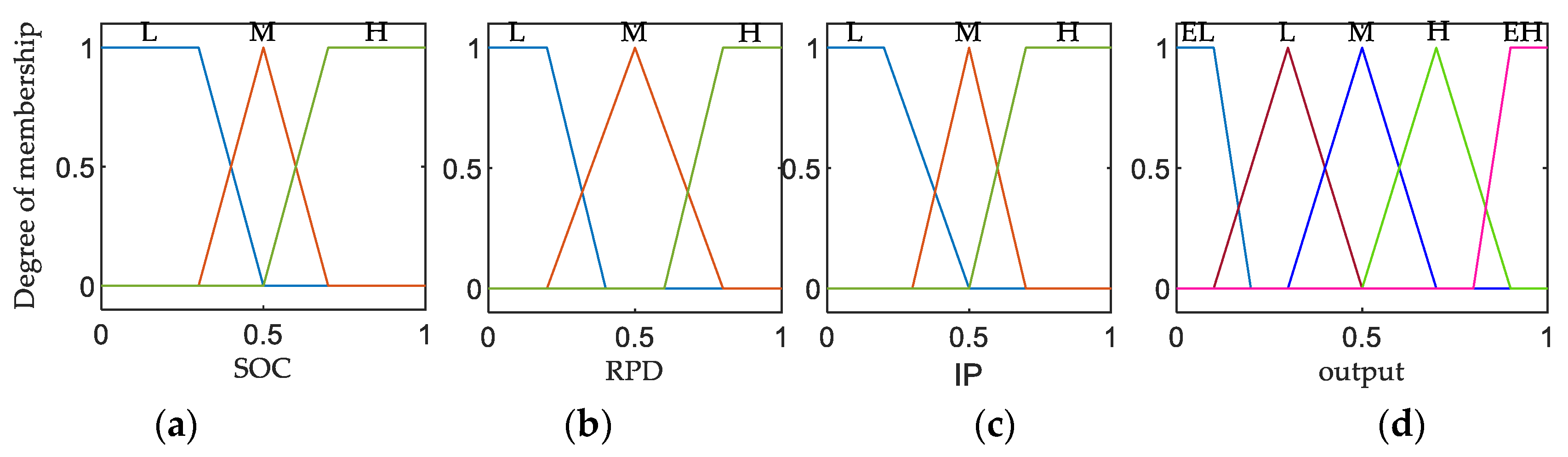
3.2. Responsive Mechanism Based on Fuzzy Rules

Firstly, based on the known remaining parking time and the remaining SOC from Section 2, and the incentive price are extracted to build the inputs for the fuzzy evaluator at each sampling period, these three factors should be normalized by Equation (15). Secondly, the fuzzification of the inputs is implemented based on the input membership functions and the output membership functions, which are shown in Figure 4a–c, respectively. Thirdly, the Mamdani fuzzy reasoning is carried out. The rule base is shown in

Table 3. Rule base and defuzzification.

If SOC Is	AND RPD Is	AND IP Is	Then the Participation of EVs DR Is	If SOC Is	AND RPD Is	AND IP Is	Then the Participation of EVs DR Is
L	L	L	EL	H	M	L	M
L	L	M	L	H	M	M	H
L	L	H	M	H	M	H	EH
M	L	L	L	L	H	L	L
M	L	M	M	L	H	M	H
M	L	H	M	L	H	H	H
H	L	L	L	M	H	L	M
H	L	M	M	M	H	M	H
H	L	H	H	M	H	H	EH
L	M	L	L	H	H	L	M
L	M	M	M	H	H	M	H
L	M	H	H	H	H	H	EH
M	M	L	L
M	M	M	M
M	M	H	H

, the fuzzy rules can be tuned with real tested results under different scenarios.

$$x^{\ast }=\frac{x-x_{\min }}{x_{\max }-x_{\min }}$$

(15)

3.3. EVA-DR Energy and Capacity

After obtaining the demand response potential of a single EV, then we construct an aggregation model of EVs’ DR. From a spatial perspective, if multiple functional blocks are powered by a certain grid node, all vehicles supplied electricity by the node are referred to herein as electric vehicle clusters which are managed by EVA. The response capability of delayed charging power and the participating discharge power at the sampling period is given by Equation (16).

$$\{\begin{array}{l}EV{A}^{del}(\mathrm{i},t)={\displaystyle \sum _{m=1}^{E{V}_{num,i}}{\rho }_m^{del}(t)·P_c^s}\\ EV{A}^{v2g}(i,t)={\displaystyle \sum _{m=1}^{E{V}_{num,i}}{\rho }_m^{v2g}(t)·P_{dis}^s}\end{array}$$

(16)

where, $E{V}_{num,i}$ is the number of EVs in the $i^{th}$ EVA cluster, $P_c^s$ and $P_{dis}^s$ are the rated charge and discharge power, respectively.

The DR capacity of an EVA and total EVAs are estimated by using Equations (17) and (18).

$$C(i,t)={\displaystyle \sum _{m=1}^{E{V}_{num,i}}(S(m,t)-{\xi }_m)·{\rho }_m(t)·E_m}$$

(17)

$$C_{tot}(t)={\displaystyle \sum _{i=1}^{N_a}C(i,t)}$$

(18)

where, $C(i,t)$ shows the DR capacity of the $i^{th}$ EVA at time t, $S(m,t)$ is the SOC of EV m at time t, ${\rho }_m(t)$ is the EVs participation in (13) and (14), ${\xi }_m$ is the limited SOC set by the EVs user and $N_a$ is the number of EVAs.

3.4. EVA-DRE Simulation Process

The steps for the proposed EVA-DRE method are provided as follows, and the simulation flowchart is described in Figure 5.

Step 1.

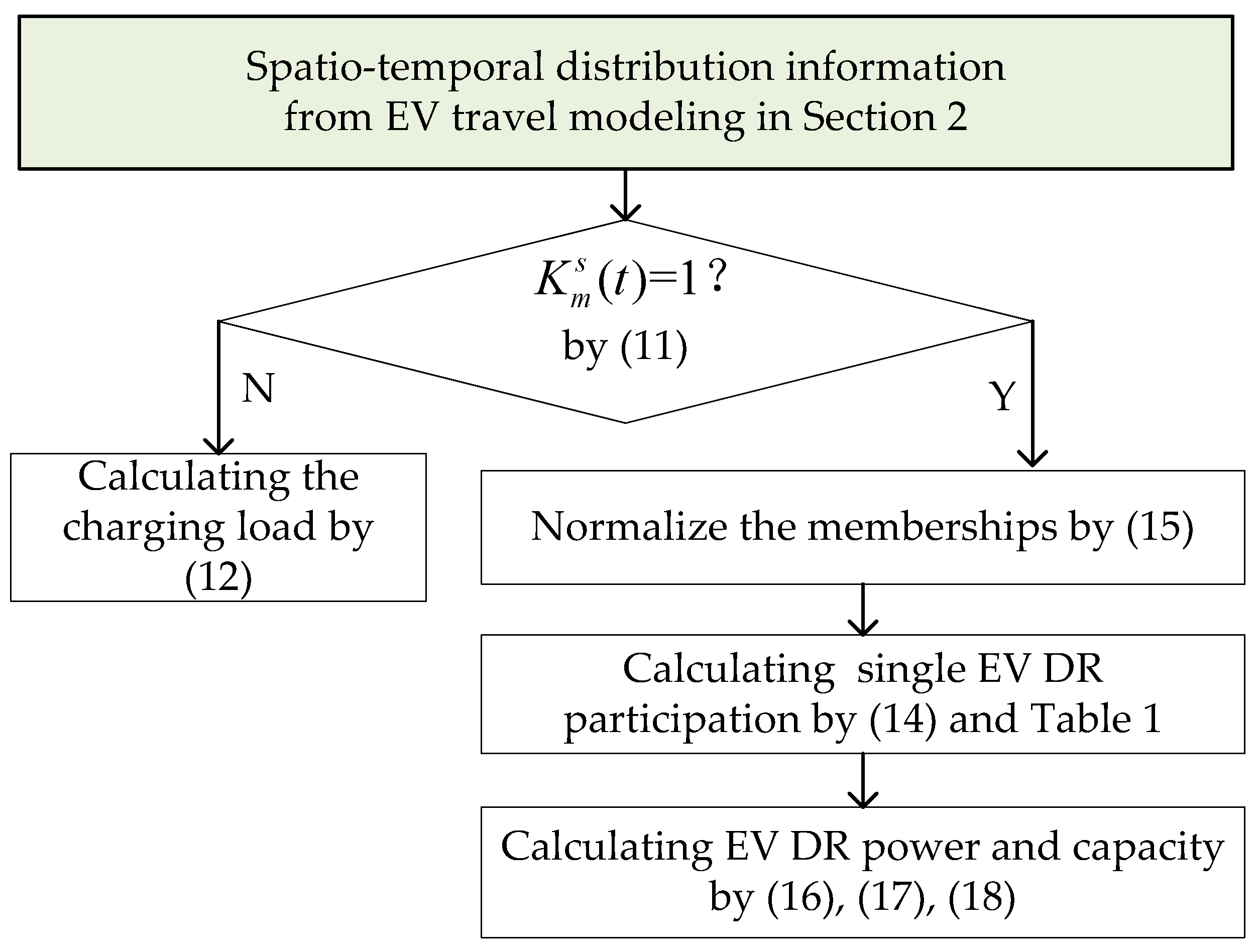
The temporal and spatial distribution of the $m^{th}$ EV and related parameters are obtained from Section 2.

Step 2.

For the participating EVs, calling the fuzzy algorithm to calculate the responsiveness of the $m^{th}$ EV.

Step 3.

Calculate the delayed charging power and V2G power and capacity of EVA according to the location of the current time of the vehicle to the corresponding EVA.

Step 4.

Accumulate the total power and capacity of EVA in the entire area.

4. Simulation Results and Analysis

In this section, we present some simulation results and the performance of the proposed method. The simulation is implemented and tested in the MATLAB software. All the results are obtained by MATLAB R2018b on a PC with Intel Core i5–4278U CPU @ 2.60 GHz, 8GB RAM memory, and 64-bit Windows 7 OS. The simulation in the case study would take 9.305 s for evaluation DR potential in each minute. In a similar fashion, to deal with large-scale dimensionality of a large scale fleet of EVs problem in [25,26,27], decentralized/distributed framework for evaluation can process.

4.1. Data Gathering and Parameter Settings

The parameters include road network information, traffic information, grid parameters, EV parameters, survey data of resident users, etc. A coupled network with 25-node road network [28] and 54-node distribution system [29] as shown in Figure 6 is used in the simulation. The road network in the region has 25 road nodes and 46 roads, 22 functional blocks, including 8 residential areas (H), 8 working places (W), 5 other functional areas (E), and 2 non-functional area (marked by Z1, Z2). Each functional area is powered by the distribution network node which is indicated by an arrow. For example, the gridlines in Figure 6 is the H7 block, which is powered by node 11.

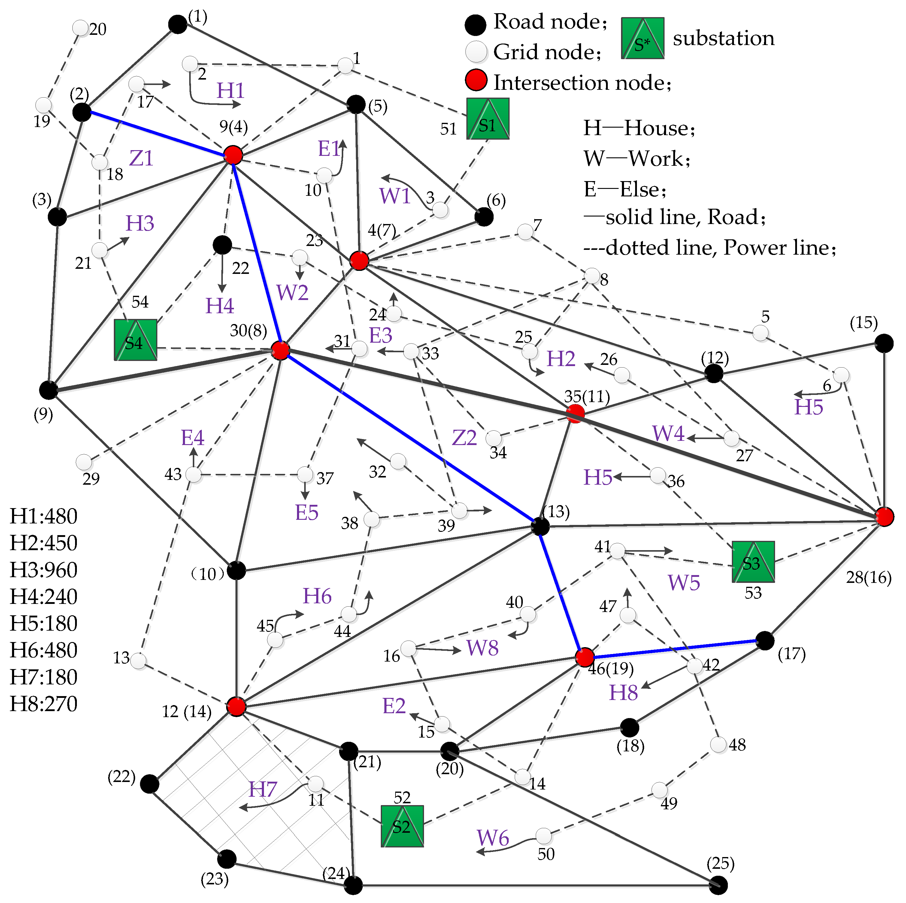
4.1.1. Detailed Road Network Information

Detailed information including links and their corresponding area, traffic light, road grade, and the length of each link are shown in

Table 4. Detailed information for the road network.

No. of Link	Original Node	Destination Node	Traffic Light	Road Grade	Length of Link	Area
1	1	5	1	3	5	0
2	1	2	1	3	4	0
3	2	3	1	3	3	0
4	2	4	1	2	4	1
5	3	4	1	3	4	0
6	3	9	1	3	4	0
7	4	5	1	3	3	0
8	4	7	1	3	5	1
9	4	8	1	2	5	1
10	4	9	1	3	7	1
11	5	6	1	3	5	0
12	5	7	1	2	5	0
13	6	7	1	3	3	0
14	7	8	1	2	3	1
15	7	11	1	3	8	1
16	7	12	1	3	9	0
17	8	9	0	1	6	1
18	8	10	1	2	6	1
19	8	11	0	1	7	1
20	8	13	1	2	7	1
21	9	10	1	3	6	0
22	10	13	1	3	6	0
23	10	14	1	2	3	0
24	11	12	1	3	2	0
25	11	13	1	3	3	1
26	11	16	0	1	7	1
27	12	15	1	3	4	0
28	12	16	1	3	4	0
29	13	14	1	3	7	0
30	13	16	1	3	7	0
31	13	19	1	2	4	0
32	14	19	1	3	7	0
33	14	21	1	3	2	0
34	14	22	1	3	4	0
35	15	16	1	3	4	0
36	16	17	1	3	4	0
37	17	18	1	3	3	0
38	17	19	1	2	3	0
39	18	20	1	3	3	0
40	19	20	1	3	3	0
41	20	21	1	3	2	0
42	20	25	1	3	4	0
43	21	24	1	3	5	0
44	22	23	1	3	3	0
45	23	24	1	3	3	0
46	24	25	1	3	8	0

. In the column of traffic light, ‘1’ denotes that there are traffic lights in the link, otherwise, there are no traffic lights in the link which is the first road grade with high free flow speed. In the column of area, ‘1’ and ‘0’ indicate the central area and other area of the city, respectively.

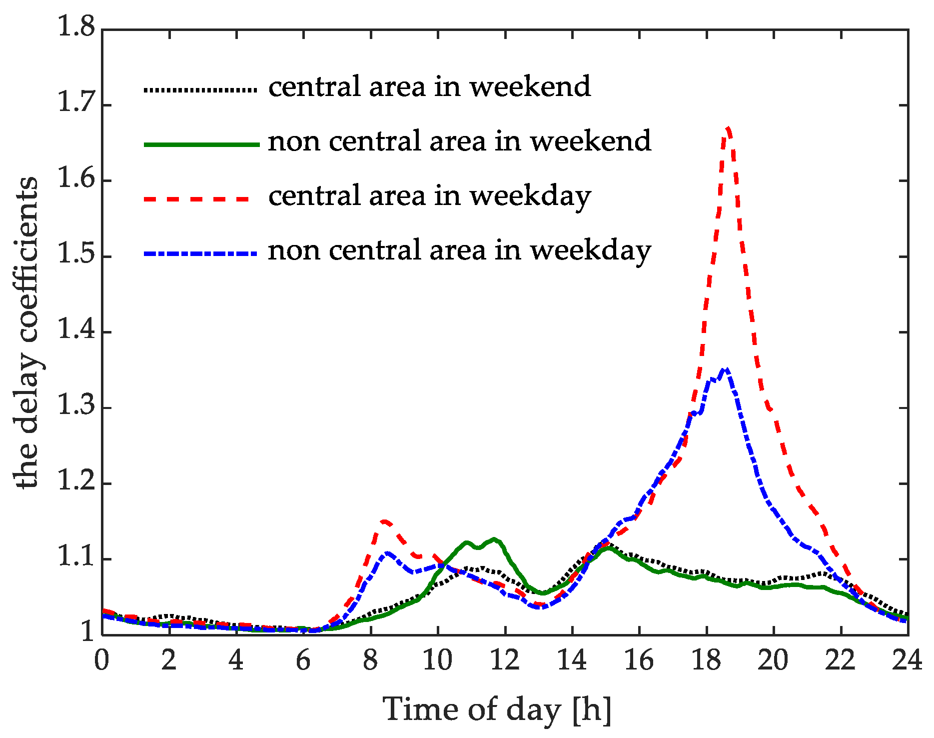
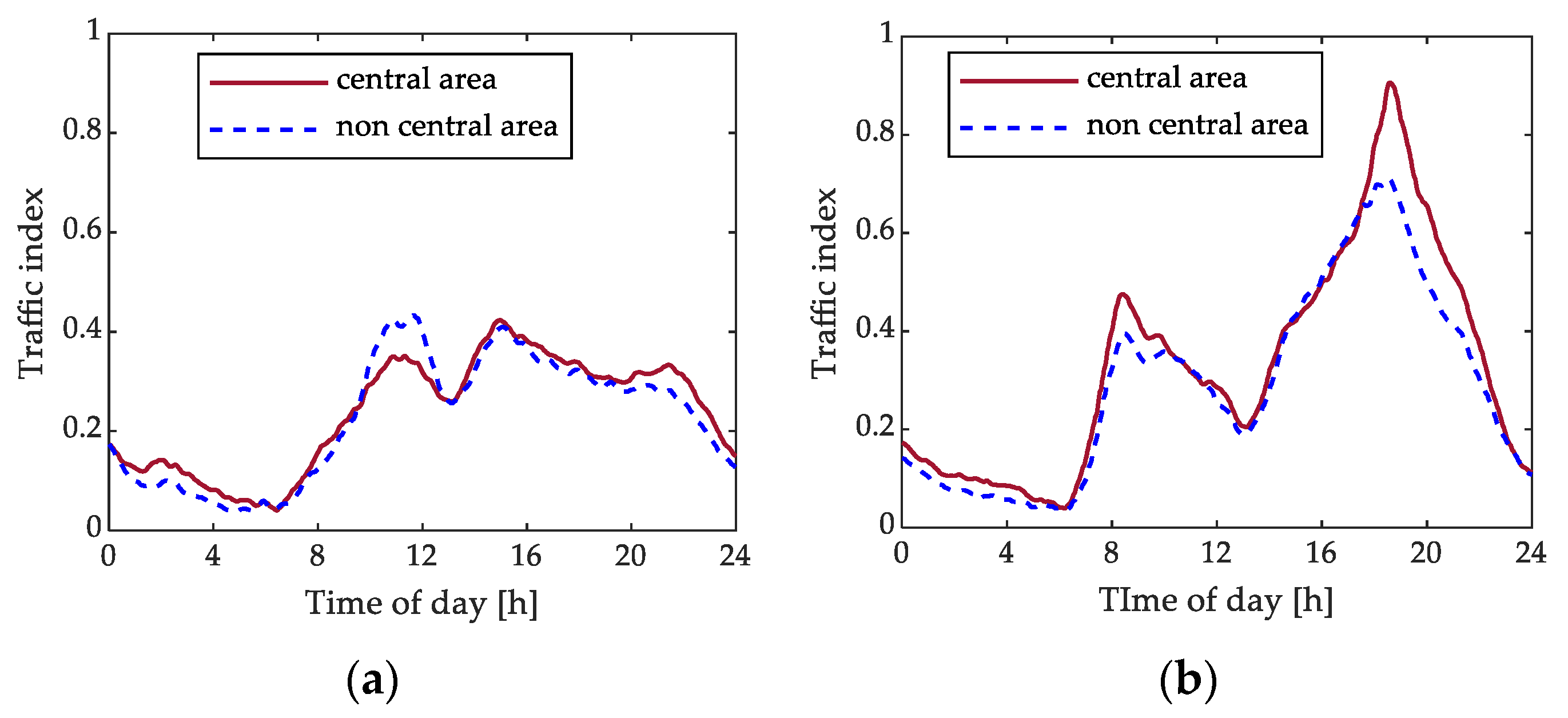
4.1.2. Traffic Information

In this paper, all the road sections are divided into four grades. In Figure 6, the thick black solid line is the fast track (FT), the blue sub-solid line is the main road (MR), and the rest are the secondary roads (SR). The branch roads (BR) are not reflected in the topological map which located in each functional area. Traffic lights are provided at the intersections of MR and SR. Different road grades have different free flow speeds, as shown in

Table 5. Free-Flow Speed in Different Urban Road Hierarchies.

Road Grade	FT	MR	SR	BR
Free-flow speed (km/h)	80	60	40	30

.

The road traffic status is divided into five levels including smooth, basically smooth, slow, medium congested, and congested. The traffic index is shown in

Table 6. Urban Traffic Index in Different Traffic Conditions.

Status	Congested	Medium Congested	Slow	Basically Smooth	Smooth
Index	0.8–1.0	0.6–0.8	0.4–0.6	0.2–0.4	0.0–0.2

.

Dynamic road network parameters are updated in real time, and the weekday and weekend traffic index of Shenzhen City in southern China are used as shown in Figure 7.

4.1.3. EVs Parameters

In our simulations, the initial and final locations of the EVs are considered to be parked in residential areas in a day. The number of EVs in each residential area (H) is shown as H1~H8 in Figure 6. The BEV Nissan Leaf, with lithium-ion battery capacity of 24 kWh, is chosen as the typical private BEV used in the simulation. The initial and limited SOC is set to 0.9 and 0.3, respectively.

4.1.4. Resident Travel Parameters

The dataset for analyzing vehicle travel behavior is mainly derived from the National Household Travel Survey (NHTS) [30]. Wednesday and Sunday data are used for weekdays and weekends, respectively. A Gaussian distribution is considered for the first trip departure time with the mean and variance presented in

Table 7. Parameters of start time and dwell time of each trip purpose for different trip chains.

	Parameters	Trip Chains Penetration		First Departure Time		Parking (Dwelling) Time
Type of Trip Chains		Workday	Weekend	Workday	Weekend	Workday		Weekend
H-W-H		40%	10%	$(457,{142}^2)$	$(550,{184}^2)$	$(544,{122}^2)$		$(504,{152}^2)$
H-E-H		20%	70%	$(635,{220}^2)$	$(744,{225}^2)$	$(222,{208}^2)$		$(144,{158}^2)$
H-W-E-H		20%	10%	$(432,{74}^2)$	$(544,{132}^2)$	$(450,{179}^2)$	$(57,{84}^2)$	$(393,{227}^2)$	$(82,{114}^2)$
H-E-W-H		20%	10%	$(601,{198}^2)$	$(712,{210}^2)$	$(550,{184}^2)$	$(179,{216}^2)$	$(94,{104}^2)$	$(102,{128}^2)$

, four types of trip chains are used for simulation as shown in Table 7.

4.1.5. Incentive Price Information

The incentive price parameter is assumed as

Table 8. Peak-Valley Time-of-Use Incentive Price (yuan/kWh).

Type	Time Slot	Incentive Price
Flat period	7:00–10:00 & 15:00–18:00 & 21:00–23:00	0.6832
Peak period	10:00–15:00 & 18:00–21:00	1.0558
Valley period	23:00-Next day 7:00	0.3105

.

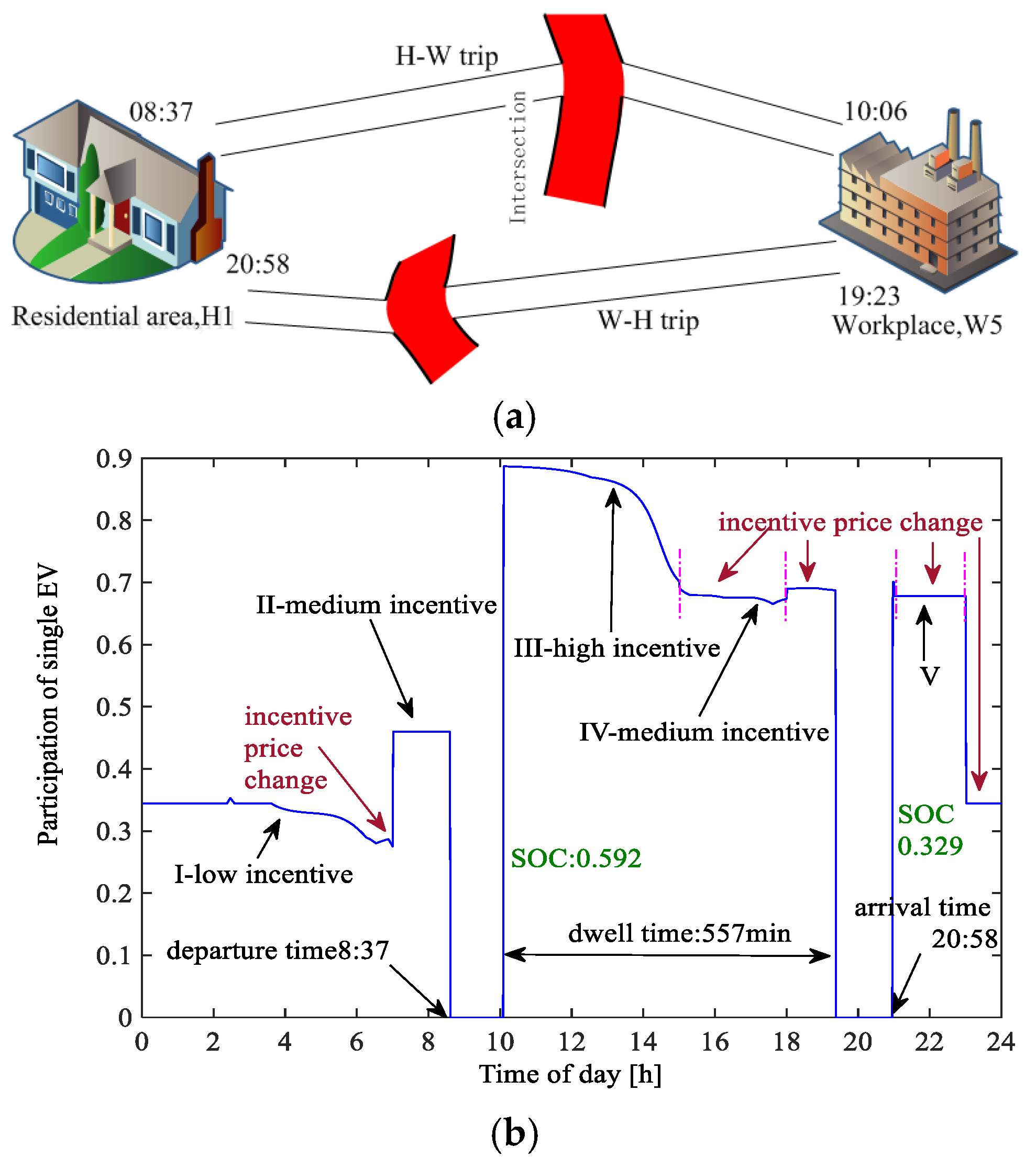
4.2. Simulation Result of a Single EV DR Potential

With the time of use incentive price in Table 8, we report the simulation result of a single vehicle in a workday as shown in Figure 8a. Considering the fuzzy participation response mechanism, its response curve is shown in Figure 8b.

It can be seen from Figure 8a that the EV arrived at the working place after leaving the house for 89 min and returned home after 557 min of parking. The return journey took 95 min. The path planned by the minimum travel time algorithm for the two trips is as shown in (19).

$$path\{\begin{array}{l}(H_1\to W_6):(1,2,4,8,11,13,19,20,25)\\ (W_6\to H_1):(25,20,19,13,8,4,2,1)\end{array}$$

(19)

where, the numbers in the brackets represent the road nodes. We can see that the round-trip routes between the two trip destinations are different. The lengths of the road segments are 34 km and 31 km, respectively, but the travel distance for calculating the power consumption is 37.01 km and 31.47 km. This is due to the large area of the functional block used in this simulation, a random length $5\times abs(2\times rand(1,1)-1)km$ is added in the calculation to reflect the mileage in each functional area. Additionally, although the ‘W-H’ trip’s driving distance was short, the traveling time was longer, which was caused by the time-consuming increase in travel time.

Figure 8b shows that the EV did not have response ability during the two-way travel period, and the lower response in the I-zone due to the low compensation of the incentive price and the closer to the departure time of the next trip. However, notwithstanding its departure time is much closer, the responsiveness in the second zone increases. This is because the increase in the incentive price has stimulated user participation.

The responsiveness of the two initial parking periods in the workplace and the residential area is relatively high, as shown in the zone III and zone V. Zone III is in a state where the incentive price is much higher, and the battery charge rate is also high. Its responsiveness is the highest throughout the day, but it gradually decreases with the declining of the remaining travel time. In zone IV, the responsiveness is further reduced due to the drop of the compensation price.

4.3. Validations

To validate the proposed method, four cases are simulated for sensitivity analysis.

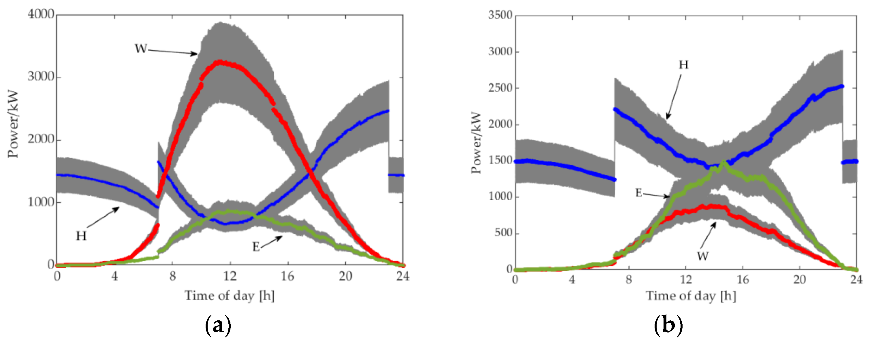
4.3.1. Workdays VS Weekends

Firstly, the simulated result for the delay coefficients of the central urban and non-central areas on weekdays and weekends are shown in Figure 9. Compared with Figure 7, the trend of the two curves is basically the same which indicates that the traffic congestion caused delays, especially during peak hours, the travel time of the central urban area is nearly 1.7 times that of the free-flow speed.

Secondly, Table 7 shows that there is a big difference in user travel pattern between weekdays and weekends. The traffic status is also significantly different as shown in Figure 7. With the incentive price of Table 8, the corresponding V2G powers of each region are shown in Figure 10.

4.3.2. DRN VS Static Road Network (SRN)

Table 9. Participation Simulation Results in Different Road Networks.

Road Network		Travel Route	Arrival Time	Arrival SOC	Participation
SRN	19:00	Path_S	20:28	0.3667	0.8806
	23:00	Path_S	23:48	0.3667	0.4143
DRN	19:00	Path_19	21:23	0.35	0.8437
	23:00	Path_23	00:31	0.3167	0.3661

displays the participation results in the dynamic road network and static road network. It is to see that the travel route, arrival time, arrival SOC, and the DR participation are different.

$$\{\begin{array}{l}\mathrm{Path}\_\mathrm{S}=(25,20,21,14,10,9,3,2,1)\\ \mathrm{Path}\_19=(25,20,21,14,10,8,4,2,1)\\ \mathrm{Path}\_23=(25,20,19,13,8,4,2,1)\end{array}$$

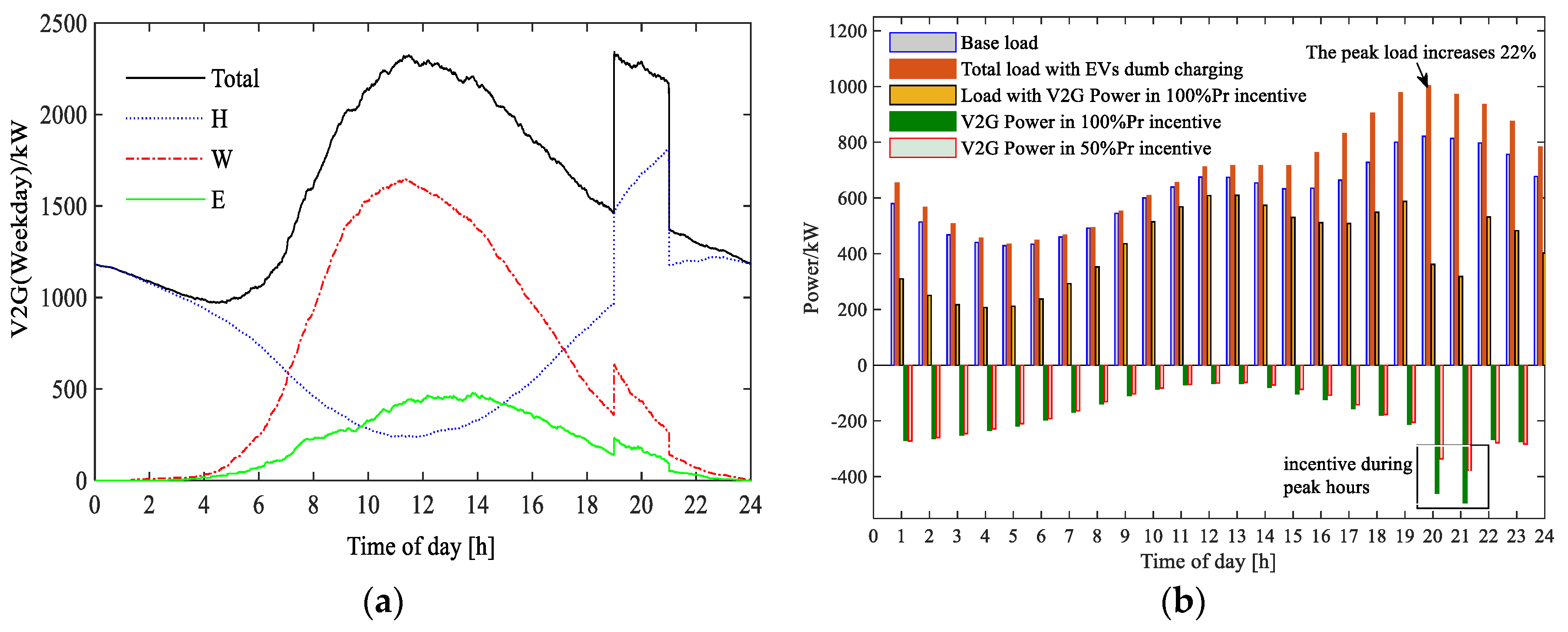
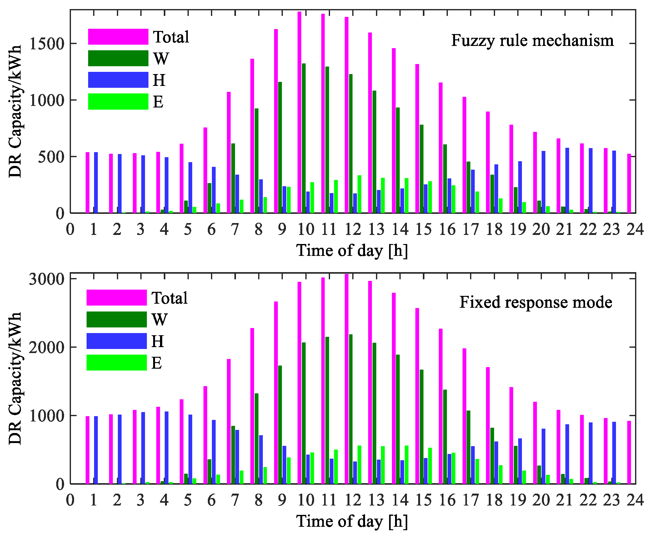
4.3.3. Different Response Mechanism

Figure 11 shows the EVA-DR capacity under the proposed EVA-DRE method and the fixed response mode that EVs will participation in DR when SOC is greater than 0.3 during the parking period. From Figure 11, the capacity of fixed response mode is much larger than the proposed method.

4.3.4. Different Incentive Price

We conducted the sensitivity analysis on the different incentive signals for the EVA-DR potential in our case study, the result is shown in Figure 12.

Taking EVs’ demand response participation in the peak load hours as an example, the V2G incentive compensation for the peak load period (19:00–21:00) is set as 50%Pr, and V2G response power result is shown in Figure 12a. It is apparent that in the case of non-peak time uncompensated electricity price incentives, the regional V2G response capacity is significantly reduced, while during the peak hours, especially in residential areas, user participation is high due to compensation incentives, and EVs usually have returned home during this period, thus, the V2G response capacity increases dramatically.

Figure 12b provides the original load curve of the residential area H4 (powered by node 22, peak load 825 kW), the load curve with EVs charging randomly, and then we simulate the response curve of EVA-DR in the H4 functional area under different incentive signals. Figure 12b shows that the ‘peak-to-peak’ effect is formed with the disordered charging during the peak load period. After the demand response project is implemented, EVA-DR effectively reduces the peak load.

5. Conclusions

We have proposed a novel quantitative evaluation method for obtaining spatio-temporal projections of demand response potential from electric vehicles. The dynamic traffic network model taking over the traffic time-varying information, trip chains, the shortest path planning algorithm, and Monte Carlo simulation are employed to derive the spatio-temporal distribution of EVs dumb charging load and battery state of charge. Investigating EV users’ willingness to participate in the DR event, a fuzzy logic-based user participation response mechanism is developed that takes into account various realistic factors such as the remaining dwell time, the remaining SOC and the incentive electricity pricing. Compared to the related literature, numerical results obtained in different cases of analysis demonstrate that the approach can achieve a reasonable spatio-temporal distribution of EVs dumb charging load, delayed charging, V2G power, and capacity. It can provide a reference for both the utilities and EVAs through the prediction of charging load and potential of electric vehicles participating in a DR event. At the same time, the proposed evaluation method can be used in regions with different sizes.

Our future work will enhance the EV user’s decision-making process considering different battery degradation functions, investigate the pricing strategy of incentive pricing, extend the simulation analysis by presenting more realistic scenarios and comparisons with other similar approaches, and finally, large-scale dimensionality of a large scale fleet of EVs will be investigated.

References

1. Boulanger, A.G.; Chu, A.C.; Maxx, S.; Waltz, D.L. Vehicle electrification: Status and issues. Proc. IEEE 2011, 99, 1116–1138. [Google Scholar] [CrossRef]
2. Islam, N.; Bloemink, J. Bangladesh’s energy crisis: A summary of challenges and smart grid-based solutions. In Proceedings of the 2018 2nd International Conference on Smart Grid and Smart Cities (ICSGSC), Kuala Lumpur, Malaysia, 12–14 August 2018; pp. 111–116. [Google Scholar]
3. Gerossier, A.; Girard, R.; Kariniotakis, G. Modeling and forecasting electric vehicle consumption profiles. Energies 2019, 12, 1341. [Google Scholar] [CrossRef]
4. Canizes, B.; Soares, J.; Costa, A.; Pinto, T.; Lezama, F.; Novais, P.; Vale, Z. Electric vehicles’ user charging behaviour simulator for a smart city. Energies 2019, 12, 1470. [Google Scholar] [CrossRef]
5. Ammous, M.; Belakaria, S.; Sorour, S.; Abdel-Rahim, A. Optimal cloud-based routing with in-route charging of mobility-on-demand electric vehicles. IEEE Trans. Intell. Transp. Syst. 2018, 1–13. [Google Scholar] [CrossRef]
6. Stüdli, S.; Crisostomi, E.; Middleton, R.; Shorten, R. A flexible distributed framework for realising electric and plug-in hybrid vehicle charging policies. Int. J. Control 2012, 85, 1130–1145. [Google Scholar] [CrossRef]
7. Carli, R.; Dotoli, M. A decentralized control strategy for optimal charging of electric vehicle fleets with congestion management. In Proceedings of the 2017 IEEE International Conference on Service Operations and Logistics, and Informatics (SOLI), Bari, Italy, 18–20 September 2017; pp. 63–67. [Google Scholar]
8. Battistelli, C. Demand response program for electric vehicle service with physical aggregators. In Proceedings of the IEEE PES ISGT Europe 2013, Copenhagen, Denmark, 6–9 October 2013; pp. 1–5. [Google Scholar]
9. Develder, C.; Sadeghianpourhamami, N.; Strobbe, M.; Refa, N. Quantifying flexibility in EV charging as DR potential: Analysis of two real-world data sets. In Proceedings of the 2016 IEEE International Conference on Smart Grid Communications (SmartGridComm), Sydney, Australia, 6–9 November 2016; pp. 600–605. [Google Scholar]
10. Acquah, M.A.; Han, S. Online building load management control with plugged-in electric vehicles considering uncertainties. Energies 2019, 12, 1436. [Google Scholar] [CrossRef]
11. Aghaei, J.; Alizadeh, M. Critical peak pricing with load control demand response program in unit commitment problem. IET Gener. Transm. Distrib. 2013, 7, 681–690. [Google Scholar] [CrossRef]
12. Rassaei, F.; Soh, W.; Chua, K. Demand response for residential electric vehicles with random usage patterns in smart grids. IEEE Trans. Sustain. Energy 2015, 6, 1367–1376. [Google Scholar] [CrossRef]
13. Erdinc, O.; Paterakis, N.G.; Mendes, T.D.P.; Bakirtzis, A.G.; Catalão, J.P.S. Smart household operation considering bi-directional EV and ESS utilization by real-time pricing-based DR. IEEE Trans. Smart Grid 2015, 6, 1281–1291. [Google Scholar] [CrossRef]
14. Izadkhast, S.; Garcia-Gonzalez, P.; Frìas, P.; Ramìrez-Elizondo, L.; Bauer, P. An aggregate model of plug-in electric vehicles including distribution network characteristics for primary frequency control. IEEE Trans. Power Syst. 2016, 31, 2987–2998. [Google Scholar] [CrossRef]
15. Liu, Y.; Gao, S.; Zhao, X.; Han, S.; Wang, H.; Zhang, Q. Demand response capability of V2G based electric vehicles in distribution networks. In Proceedings of the 2017 IEEE PES Innovative Smart Grid Technologies Conference Europe (ISGT-Europe), Torino, Italy, 26–29 September 2017; pp. 1–6. [Google Scholar]
16. Wang, J.; Shi, Y.; Zhou, Y. Intelligent demand response for industrial energy management considering thermostatically controlled loads and EVs. IEEE Trans. Ind. Inform. 2018, 1. [Google Scholar] [CrossRef]
17. Şengör, I.; Erdinç, O.; Yener, B.; Taşcikaraoglu, A.; Catalão, J.P.S. Optimal energy management of EV parking lots under peak load reduction based dr programs considering uncertainty. IEEE Trans. Sustain. Energy 2018, 1. [Google Scholar] [CrossRef]
18. Peng, W.; Dong, G.; Yang, K.; Su, J. A random road network model and its effects on topological characteristics of mobile delay-tolerant networks. IEEE Trans. Mob. Comput. 2014, 13, 2706–2718. [Google Scholar] [CrossRef]
19. Chen, L.; Nie, Y.; Zhong, Q. A model for electric vehicle charging load forecasting based on trip chains. Trans. China Electrotech. Soc. 2015, 30, 216–225. [Google Scholar]
20. Gong, L.; Cao, W.; Liu, K.; Zhao, J.; Li, X. Spatial and temporal optimization strategy for plug-in electric vehicle charging to mitigate impacts on distribution network. Energies 2018, 11, 1373. [Google Scholar] [CrossRef]
21. Li, M.; Lenzen, M.; Keck, F.; McBain, B.; Rey-Lescure, O.; Li, B.; Jiang, C. GIS-based probabilistic modeling of BEV charging load for Australia. IEEE Trans. Smart Grid 2018, 1. [Google Scholar] [CrossRef]
22. Castillo, E.; Calviño, A.; Sánchez-Cambronero, S.; Lo, H.K. A multiclass user equilibrium model considering overtaking across classes. IEEE Trans. Intell. Transp. Syst. 2013, 14, 928–942. [Google Scholar] [CrossRef]
23. Lu, C.; Zhao, F.; Hadi, M. A travel time estimation method for planning models considering signalized intersections. In Proceedings of the ICCTP 2010: Integrated Transportation Systems: Green, Intelligent, Reliable, Beijing, China, 4–8 August 2010; pp. 1993–2000. [Google Scholar]
24. Amini, M.H.; Karabasoglu, O. Optimal operation of interdependent power systems and electrified transportation networks. arXiv, 2018; arXiv:1701.03487. [Google Scholar]
25. Ma, Z.; Callaway, D.S.; Hiskens, I.A. Decentralized charging control of large populations of plug-in electric vehicles. IEEE Trans. Control Syst. Technol. 2013, 21, 67–78. [Google Scholar] [CrossRef]
26. Parise, F.; Colombino, M.; Grammatico, S.; Lygeros, J. Mean field constrained charging policy for large populations of Plug-in Electric Vehicles. In Proceedings of the 53rd IEEE Conference on Decision and Control, Los Angeles, CA, USA, 15–17 December 2014; pp. 5101–5106. [Google Scholar]
27. Carli, R.; Dotoli, M. A distributed control algorithm for waterfilling of networked control systems via consensus. IEEE Control Syst. Lett. 2017, 1, 334–339. [Google Scholar] [CrossRef]
28. Hodgson, M.J. A flow-capturing location-allocation model. Geogr. Anal. 1990, 22, 270–279. [Google Scholar] [CrossRef]
29. Miranda, V.; Ranito, J.V.; Proenca, L.M. Genetic algorithms in optimal multistage distribution network planning. IEEE Trans. Power Syst. 1994, 9, 1927–1933. [Google Scholar] [CrossRef]
30. U.S. Department of Transportation Federal Highway Administration. 2017 National Household Travel Survey; U.S. Department of Transportation Federal Highway Administration: Washington, DC, USA, 2017.
Figure 1. Scheme of proposed EVA-DRE method.
Energies 12 01981 g001
Figure 2. The daily trip chains.
Energies 12 01981 g002
Figure 3. Flowchart of EV travel model.
Energies 12 01981 g003
Figure 4. The membership functions. (a) State-of-charge (SOC); (b) Rest parking duration (RPD); (c) Incentive price (IP); (d) Output membership functions (EV-DR participation).
Energies 12 01981 g004
Figure 5. Flowchart of EVA-DRE method.
Energies 12 01981 g005
Figure 6. Topology coupled road network and distribution network.
Energies 12 01981 g006
Figure 7. Traffic index of (a) weekend; (b) weekday.
Energies 12 01981 g007
Figure 8. Probability of EV DR. (a) ‘H-W-H’ trip chain. (b) the demand response of a single EV.
Energies 12 01981 g008
Figure 9. Delay coefficients under different traffic index.
Energies 12 01981 g009
Figure 10. V2G Power demand response distribution of EVA-DR in weekday and weekend (a) weekday; (b) weekend.
Energies 12 01981 g010
Figure 11. EVA-DR capacity expectation with different mechanism.
Energies 12 01981 g011
Figure 12. EVA-DR under different incentives. (a) V2G power expectation under high incentive compensation of peak hours (with 33% penetration); (b) EV charge randomly and different peak price incentives (H4: 240 EVs).
Energies 12 01981 g012