A Data-Driven Workflow Approach to Optimization of Fracture Spacing in Multi-Fractured Shale Oil Wells

Abstract

A data-driven workflow approach is presented in this study for optimizing fracture spacing of multifractured horizontal wells (MFHW) in shale oil reservoirs. The workflow employs a simple well productivity model for the initial design of hydraulic fracturing well completions. This provides a transparent approach to the identification of key fracturing parameters affecting well productivity. The workflow uses transient pressure or production data to identify fracture interference. This offers a reliable and cost-effective means for assessment of well production potential in terms of optimization of fracture spacing in the MFHW. Result of a field case study indicated that three wells were drilled in an area with dense natural fractures, and the fracture spacing of MFHW in this area was short enough to effectively drain the stimulated reservoir volume (SRV), while the other three wells were drilled in an area with less natural fractures, and the fracture spacing of MFHW in this area could be shortened to double well productivity.

1. Introduction

Thanks to multifractured horizontal well (MFHW) technology, development of shale oil fields in the past five years has made United States energy self-sufficient. However, the results of the technology in other regions of the world are mixed. This is partially attributed to inadequate effort in optimizing a completed design of MHFW.

Modern MFHW techniques include simul frac, zipper frac, and modified zipper frac. Simul frac creates simultaneous hydraulic fractures in symmetric stages in two wells. Zipper frac creates alternate hydraulic fractures in symmetric stages in two wells. Modified zipper frac creates hydraulic fractures in nonsymmetric stages in two alternate wells [1]. These fracturing techniques create symmetric, transverse fractures of ideally the same length and spacing. This common structure of multifractured horizontal wells allows for using general mathematical models to predict well productivity in the stage of well completion design.

The available methods for predicting shale well productivity include analytical transient flow models [2,3,4,5,6] and numerical computer models [7,8,9,10,11]. Analytical transient flow models are mostly used in pressure transient test analyses rather than in optimizing well completion design. Numerical computer models are flexible in handling systems with nonsymmetrical fractures and multiphase flows [12]. In addition to model complicity, the uncertainty in locations of natural fractures is a concern regarding the accuracy of computer simulation results. Based on the work of Guo et al. [13], Zhang et al. [14] presented an analytical solution for estimating long-term productivity of multifractured shale gas wells by coupling the linear flow in the reservoir and the linear flow in hydraulic fractures. Li et al. [15] extended the analytical solution to shale oil wells and validated the solutions with field data from an oil well and a gas well.

The results of MFHW technology in different regions of the world are inconsistent. This is believed partially because of the lack of optimization of MHFW parameters, especially fracture spacing. Optimization of such spacing is considered as one of the most critical steps in enabling economic of horizontal wells and requires a lot of attention [7]. A data-driven workflow procedure, combined with simple well productivity models, is presented in this paper for fracture spacing optimization. This workflow procedure has the advantage of using a simple analytical well productivity model driven by real production data, making it a practical approach to optimize multistage fracturing of horizontal wells in shale oil reservoirs.

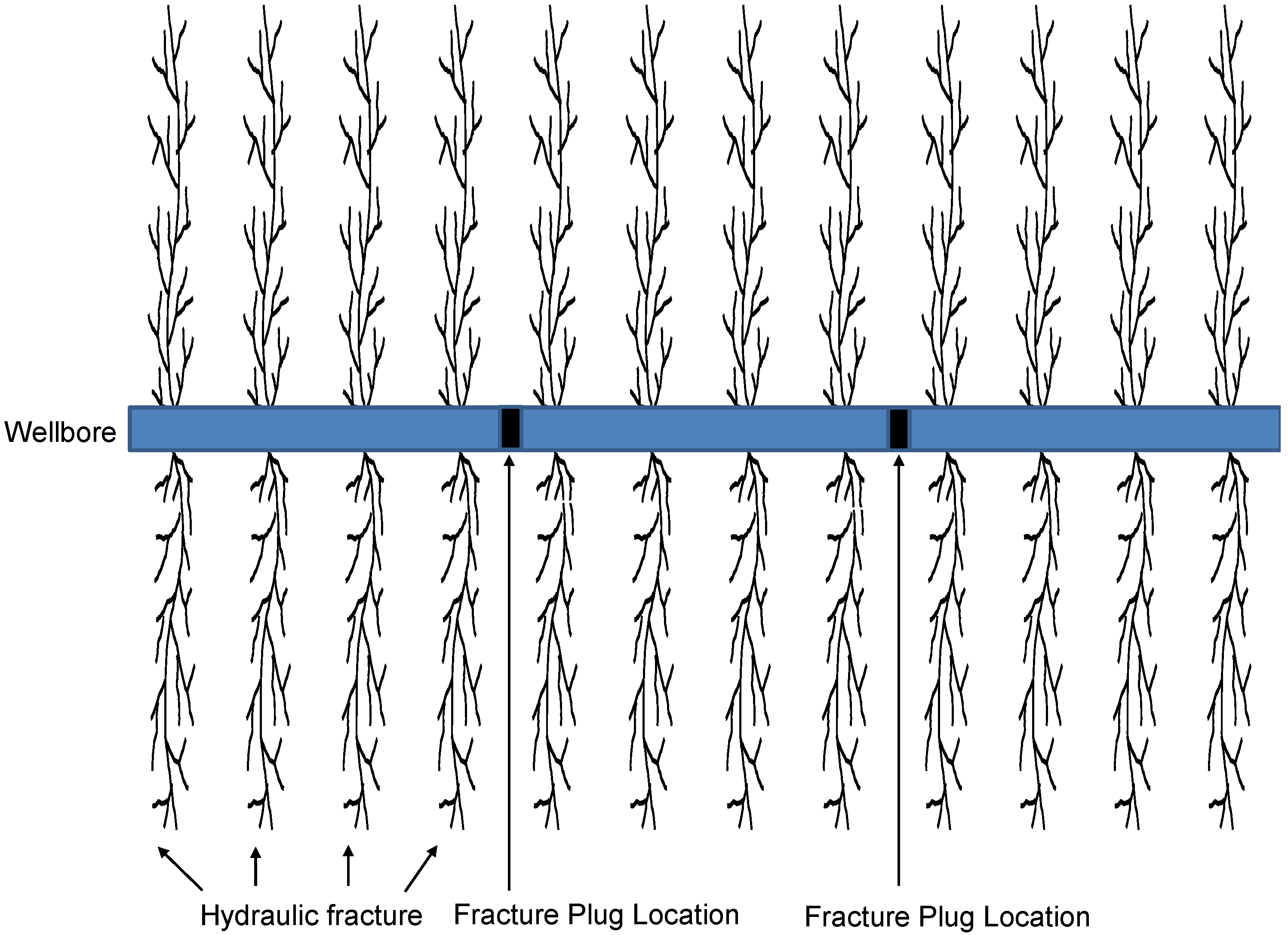
2. Concept of Fracture Spacing

Modern shale oil and gas horizontal wells are mostly fractured in multiple stages utilizing plug and perf methodology, where the stages are separated by frac plugs set inside the casing. Perforation clusters are created for each stage. The explosive energy during perforating should induce microcracks from the perforations [16]. When fracturing fluid is forced to go through the perforations, multiple fractures may be initiated from these microcracks or other heterogeneities such as natural fractures, drilling-induced fractures, rock texture, orientation and magnitude of formation stresses, etc. The orientations of fractures near the wellbore area are complicated because the wellbore and perforations alter the state of stress in this area [16].

A number of fracture propagation mechanisms may exist. Fractures may re-orientate from the perforations towards preferred fracture planes, owing to stress anisotropy. Fractures may also interact with and merge to natural fractures if the latter exists. As a result, multiple and tortuous fractures are anticipated near the wellbore area. When these initial fractures propagate away from the wellbore area, they may converge or diverge depending on stress field and natural fractures. Branching due to shale heterogeneities may develop from a single fracture. All fractures initiated from a perforation cluster should form a hydraulic fracture in the plane normal to the minimum principal stress to achieve the minimum strain energy in the shale. Twelve hydraulic fractures created from 12 perforation clusters are depicted in Figure 1. The fracture spacing is defined in this study as the distance between the centerlines of two adjoined hydraulic fractures, which are expected to be equal to the distance between the two adjoined perforation clusters.

Although well productivity models, such as those presented by Zhang et al. [14] and Li et al. [15], suggest reducing fracture spacing for maximizing well productivity, short spacing may cause early interferences between fractures as a result of fracture branching. Whether early interference exists or not depends on local geological conditions, especially natural fractures and local rock stress fields. Fracture interference can be identified by pressure transient data analyses and/or production rate transient data analyses.

3. Workflow for Optimization

The proposed workflow to optimize fracture spacing is based on industry practice [16], with the addition of data analysis, to identify fracture interference. It is summarized in the following steps:

• Design a fracturing job for the first well in the area for a desirable production rate using a well productivity model. Fracture spacing is selected based on horizontal wellbore length, volumes of fracturing fluid and proppant, and completion tools.
• Execute the fracturing job using the designed fracture spacing and other parameters.
• Run a pressure transient test on the well if possible, and put the well into production.
• Perform transient pressure or transient production rate data analyses to identify fracture interference.
• If well completion permits, refracture the well based on the identified fracture interference.
• Modify the well completion design including the fracturing treatment design and/or the spacing between perforation clusters for the next well on the basis of fracture interference in the previous well.

Some of these workflow steps are further outlined in the subsections that follow.

3.1. Fracturing Design

The physics of fluid flow in shale oil reservoirs is adequately described in the literature. The assumptions employed in this study were oversimplified, as the desorption of hydrocarbon from rock matrix and non-Darcy flow were not considered. However, it is a fact that pressure transient and production data support the mathematical models derived from Darcy’s law. This implies that fluid flow in shale oil reservoirs is dominated by Darcy’s law.

Fracturing design can be guided by mathematical models derived from Darcy’s law for shale gas and oil well production under pseudosteady flow conditions. For multifractured horizontal oil wells, Li et al.’s model for oil production rate is expressed as [15]:

$$q_o=\frac{5.91\times {10}^{-3}{n}_f{k}_m{h}_f\left(\overline{p}-p_w\right)}{B_o{\mu }_o{S}_f\sqrt{c}\left(\frac{1}{1-e^{-\sqrt{c}{x}_f}}-\frac{1}{3x_f\sqrt{c}}\right)},$$

(1)

where c is expressed as:

$$c=\frac{96k_m}{k_{f}w{S}_f},$$

(2)

where q_o is the well production rate in stb/d, n_f is the number of perforation clusters (hydraulic fractures), k_m is the matrix permeability in md, h_f is the fracture height in ft, $\overline{p}$ is the average formation pressure in psia, p_w is the wellbore pressure in psia, μ_o is the oil viscosity in cp, B_o is the oil formation factor in rb/stb, S_f is the fracture spacing in ft, e is an exponential function, x_f is the hydraulic fracture half-length in ft, k_f is the fracture permeability in md, and w is the average fracture width in inches.

Substituting Equation (2) into Equation (1) yields:

$$q_o=\frac{6.03\times {10}^{-4}{n}_f{h}_f\left(\overline{p}-p_w\right)}{B_o{\mu }_o\left(\frac{1}{1-e^{-\sqrt{c}x}}-\frac{1}{3x_f\sqrt{c}}\right)}\sqrt{\frac{k_m{k}_{f}w}{S_f}}.$$

(3)

Although Equation (3) shows that maximum well productivity can be obtained by optimizing the effects of the number of hydraulic fractures, hydraulic fracture spacing, and hydraulic fracture width, this is not true in reality as fracture complexity and additional factors such as frac hits also exist. As pointed out by Potapenko et al. [17], in most of the unconventional reservoirs where the majority of multistage wells are drilled, the fracture geometry is quite complex and interaction between fractures starts very early. In this case, spacing between perforation clusters should not have much impact on well productivity. However, in situations where a significant portion of hydraulic fractures is damaged during well startup, resulting in disconnections of such fractures from the wellbore, having small spacing between perforation clusters still appears to be beneficial because disconnected fractures still may contribute to production through other nondamaged perforation clusters [17]. The issues of fracture complexity, interaction, and disconnection are quite difficult to consider in mathematical modeling because there is a lack of data to explicitly describe their configurations and dynamics [18]. These complication issues are assumed to be negligible in the analysis that follows.

For a given horizontal wellbore length L, well operators tend to increase the number of perforation clusters during the well completion optimization process. It brings some additional considerations about fracture length, the number of frac stages, and the volume of frac treatment. The number of clusters is expressed as:

$$n_f=\frac{L}{S_f}.$$

(4)

For a given total volume of fracture proppant V_f in ft³, the following material balance holds:

$$V_f=n_f\left(2x_f\right)\left(\frac{w}{12}\right)h_f.$$

(5)

It should be mentioned that w in Equation (4) is in inches, and V_f is the bulk volume (not the physical volume) of proppant.

Substituting Equation (4) into Equation (5) and rearranging the latter gives:

$$w=\frac{6V_f{S}_f}{x_f{h}_{f}L}.$$

(6)

Substituting Equations (4) and (6) into Equation (3) results in:

$$q_o=\frac{1.48\times {10}^{-3}\left(\overline{p}-p_w\right)}{B_o{\mu }_o{S}_f\left(\frac{1}{1-e^{-\sqrt{c}{x}_f}}-\frac{1}{3x_f\sqrt{c}}\right)}\sqrt{\frac{k_m{k}_f{h}_f{V}_{f}L}{x_f}}.$$

(7)

The average reservoir pressure is [15]:

$$\overline{p}=p_e-\frac{p_e-p_w}{3x_f\sqrt{c}}\left(1-e^{-\sqrt{c}{x}_f}\right),$$

(8)

where p_e is the reservoir pressure in psia.

It can be shown that in the practical ranges of parameters the sum of the two terms in the bracket in the denominator is very close to unity. Therefore, if fracture spacing is reduced, both the number of clusters and the total fracture surface will increase. Under the assumption of reservoir linear flow (RLF) with infinite fracture conductivity, the well production rate is proportional to the total fracture surface area. This supports the concept of massive volume fracturing where many clusters with the shortest possible spacings are used for pumping massive proppant into the created hydraulic fractures.

Although cluster spacing should be theoretically as low as possible for maximizing well productivity, a minimum required cluster spacing (MRCS) has to be considered in practice if temporal change and well lifetime are not considered. MRCS is controlled by (1) well completion design and equipment limitations and (2) hydraulic fracture interference. In well completion design, frac plugs and perforation clusters themselves are spaced apart, and casing couplings have to be avoided in perforation clusters. Perf gun can carry a limited number of charges, which are used for the creation of perf clusters. Adding a higher number of perf clusters may require a higher number of perf trips, which impacts overall cost and the operational efficiency. For the concern of hydraulic fracture interferences, sever connections of hydraulic fractures from different perforation clusters are usually not desirable, although overlapping of the frac networks from different perforation clusters may be quite beneficial to well productivity. This interference can be assessed using transient pressure or transient production data analysis.

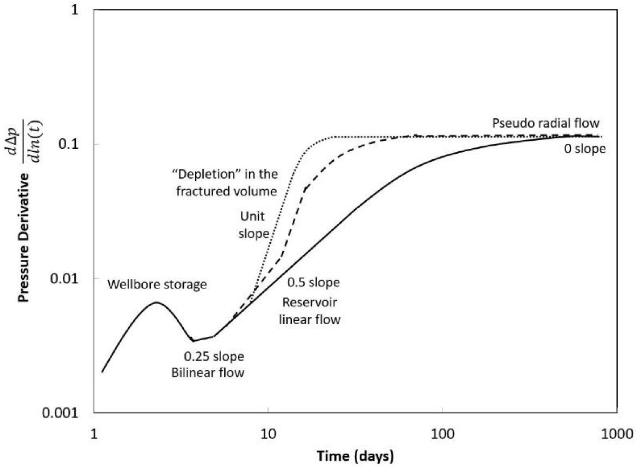
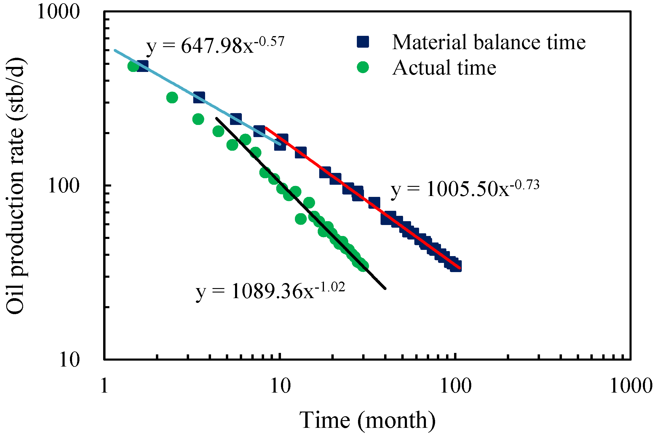
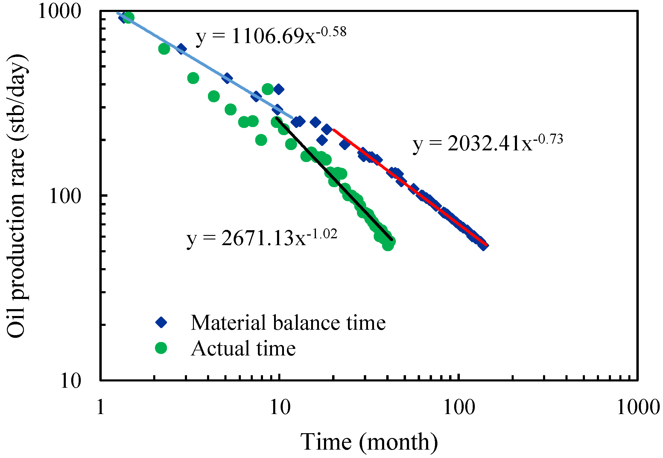
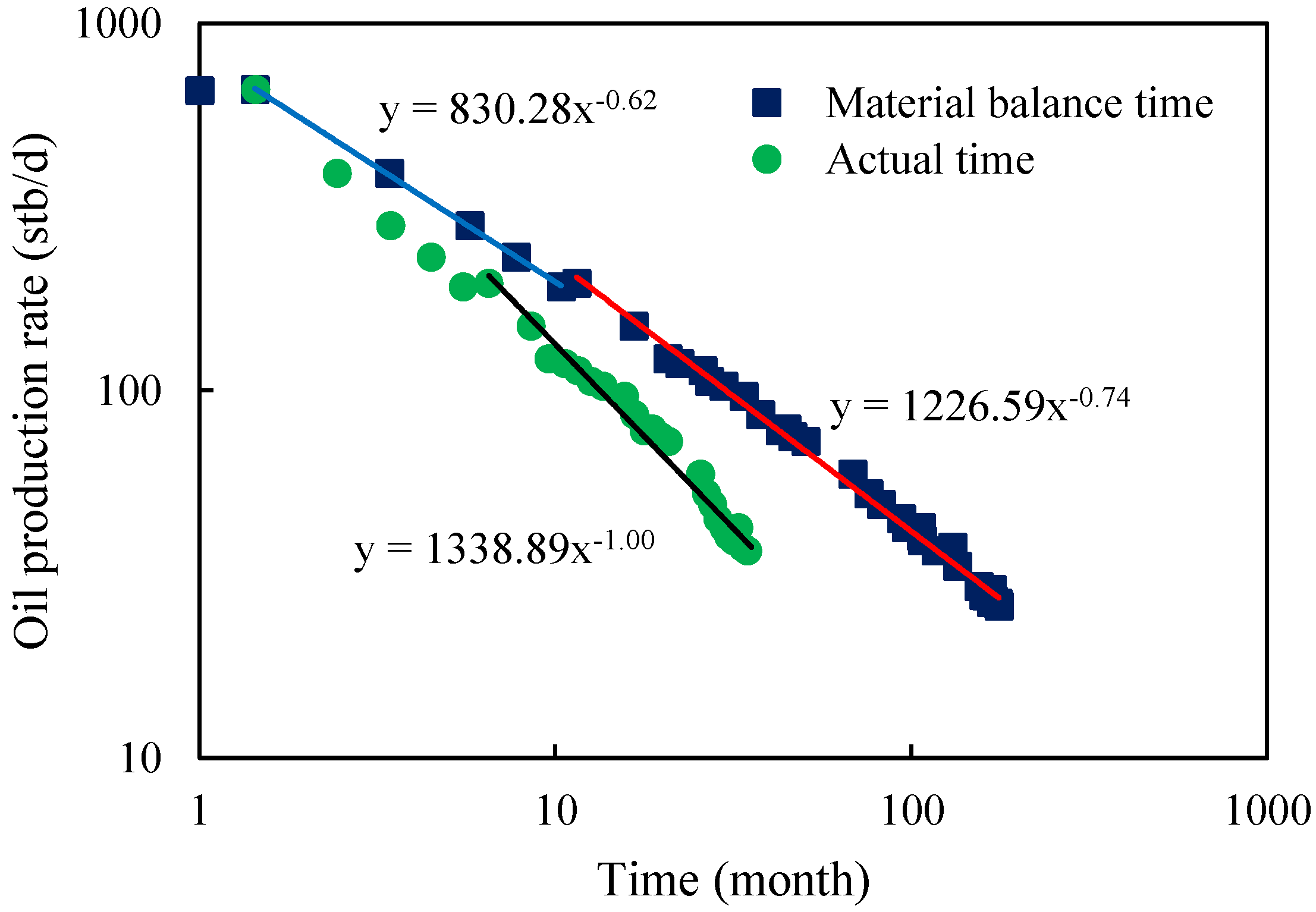
3.2. Transient Pressure Analysis for Fracture Interference Identification

The theoretical basis of pressure transient data analysis can be found in numerous references [19,20,21]. Modern computer software packages available for pressure transient and production data analyses include F.A.S.T. WellTest [22] and PanSystem [23]. Applications of the pressure transient data analysis theory to shale gas and oil wells are shown by a number of investigators such as Shan et al. [24], Pang et al. [25], and He et al. [26]. Figure 2 presents a diagnostic plot of pressure transient data for flow regime identification where the vertical axis is the pressure derivative defined by:

$$p^{\prime }=\frac{d\Delta p}{d\ln t},$$

(9)

where Δp is the pressure change, defined as reservoir pressure minus flowing bottom hole pressure for drawdown tests and shut-in bottom pressure minus the last flowing bottom hole pressure before shutting-in for pressure buildup tests. t is the test time defined as the flow time for drawdown tests and shut-in time for pressure buildup tests.

Mathematical models describing reservoir transient linear flow to fractures are found in the literature [27,28]. For a well with infinite conductivity fractures, reservoir linear flow (RLF) can be identified by the half-slope of the pressure derivative data versus time data plotted on a log–log scale. For a well with finite conductivity fractures, a bilinear flow may occur in the fracture and in the formation matrix during the initial stages. Pressure derivative data versus time data plotted on a log–log scale should show a straight line with a slope of 0.25 [29]. After the pressure change propagates to the midline between fractures, pressure derivative data versus time data plotted on a log–log scale should show a straight line with the unit slope for boundary dominated flow (BDF) during the “depletion” in the fractured volume. If a slope value greater than 0.5 is observed soon after wellbore storage, interference between fractures is indicated.

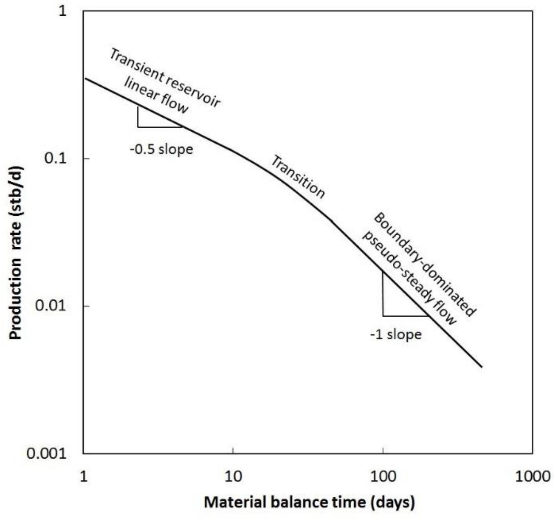
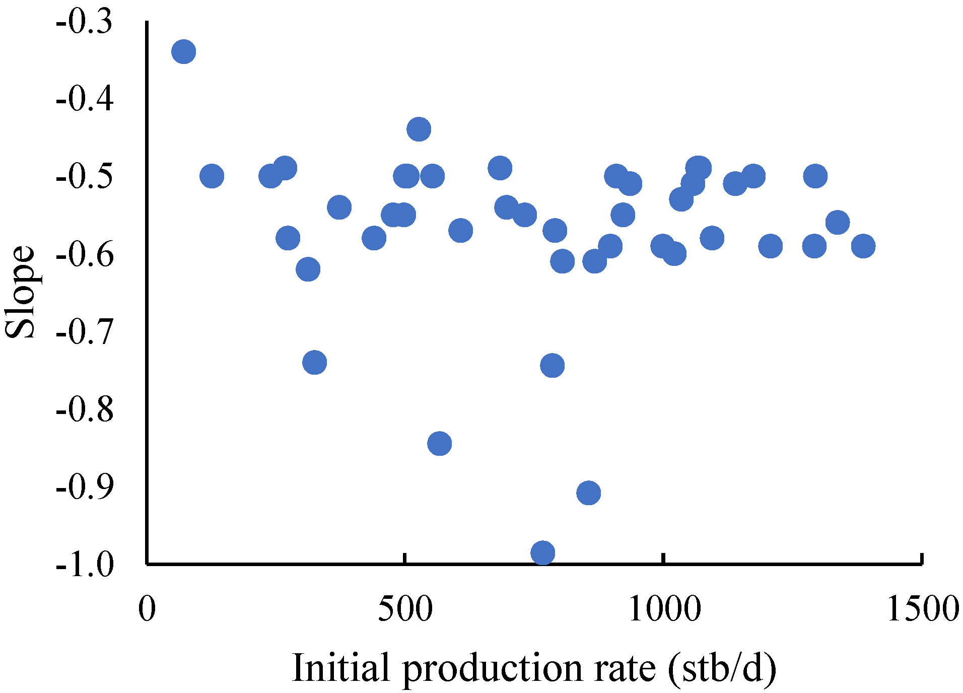
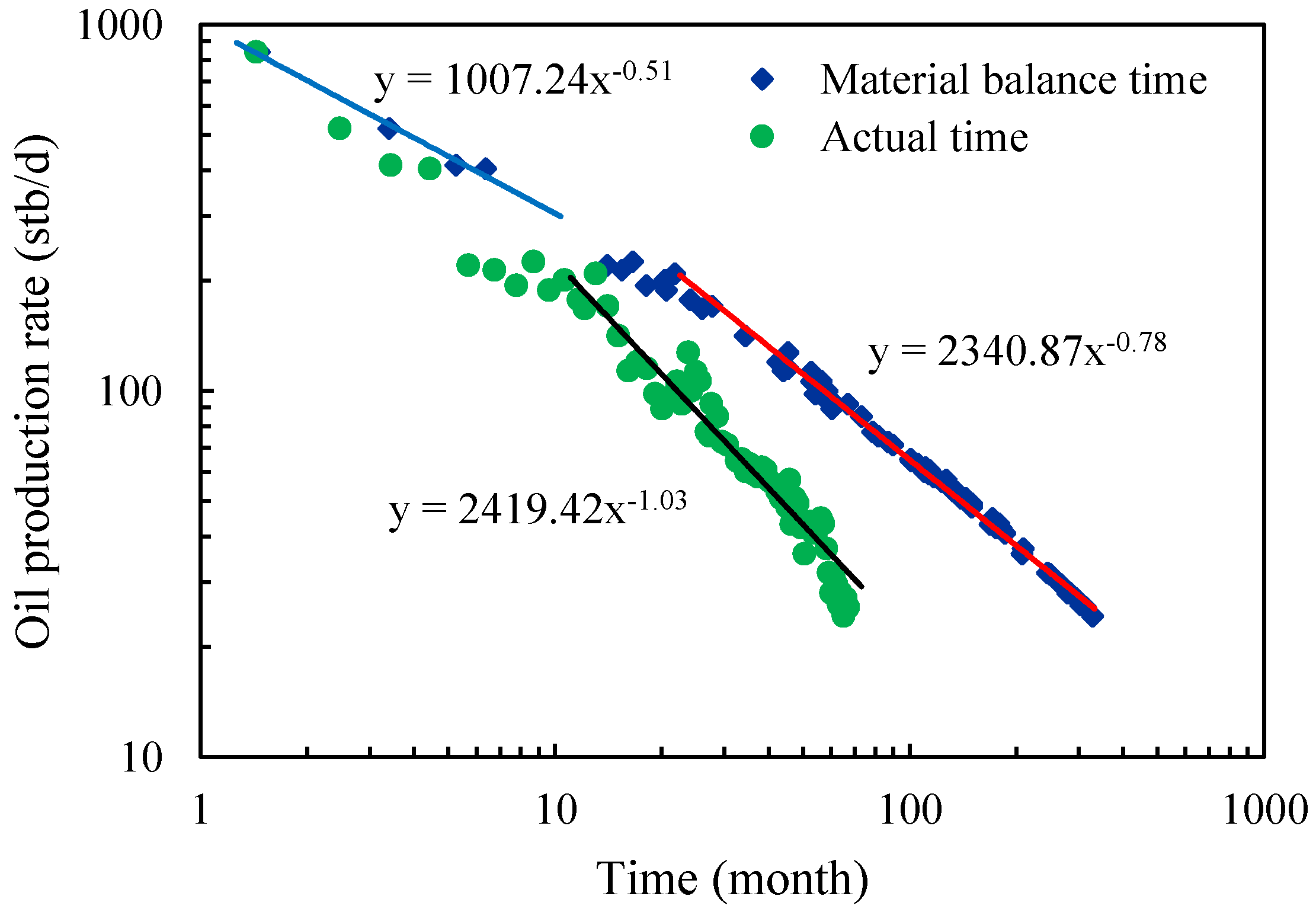
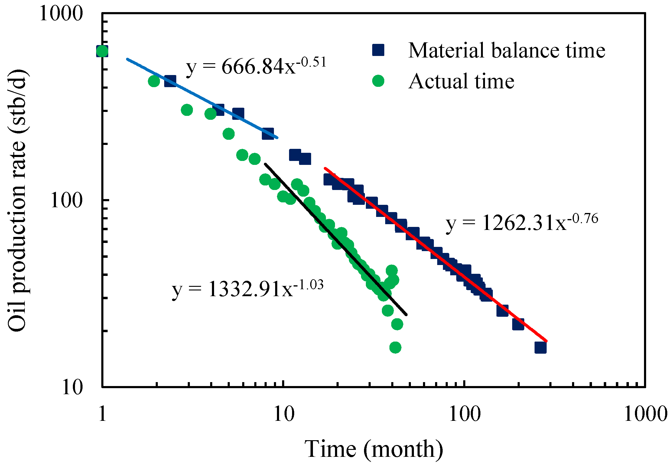
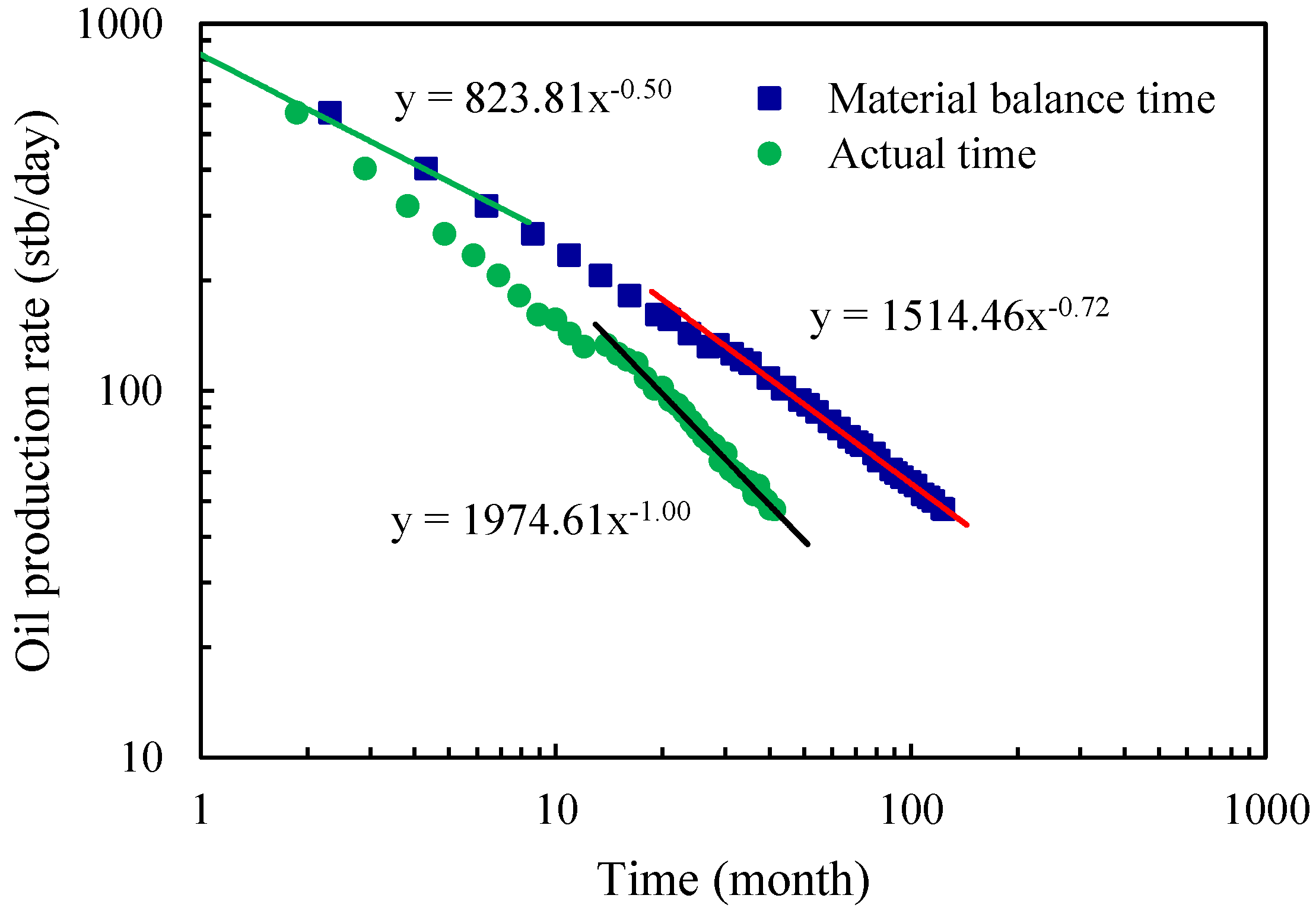
3.3. Transient Rate Analysis for Fracture Interference Identification

Applications of the transient production data analysis theory to shale oil wells are also demonstrated by previous investigators [30,31,32]. Figure 3 shows a diagnostic plot of rate transient data for flow regime identification. For a well with infinite conductivity fractures, the production rate data versus time data plotted on a log–log scale should show a straight line with a slope of −0.5 during the RLF. For a well with finite conductivity fractures, a bilinear flow may occur in the fracture and in the formation matrix during the initial stages. Rate data versus time data plotted on a log–log scale should show a straight line with a slope of −0.25. After the depth of investigation propagates to the midline between fractures, rate data versus time data plotted on a log–log scale should show a straight line with a slope of −1 for BDF. If a slope value between −0.5 and −1 is observed early on, interference between fractures is indicated.

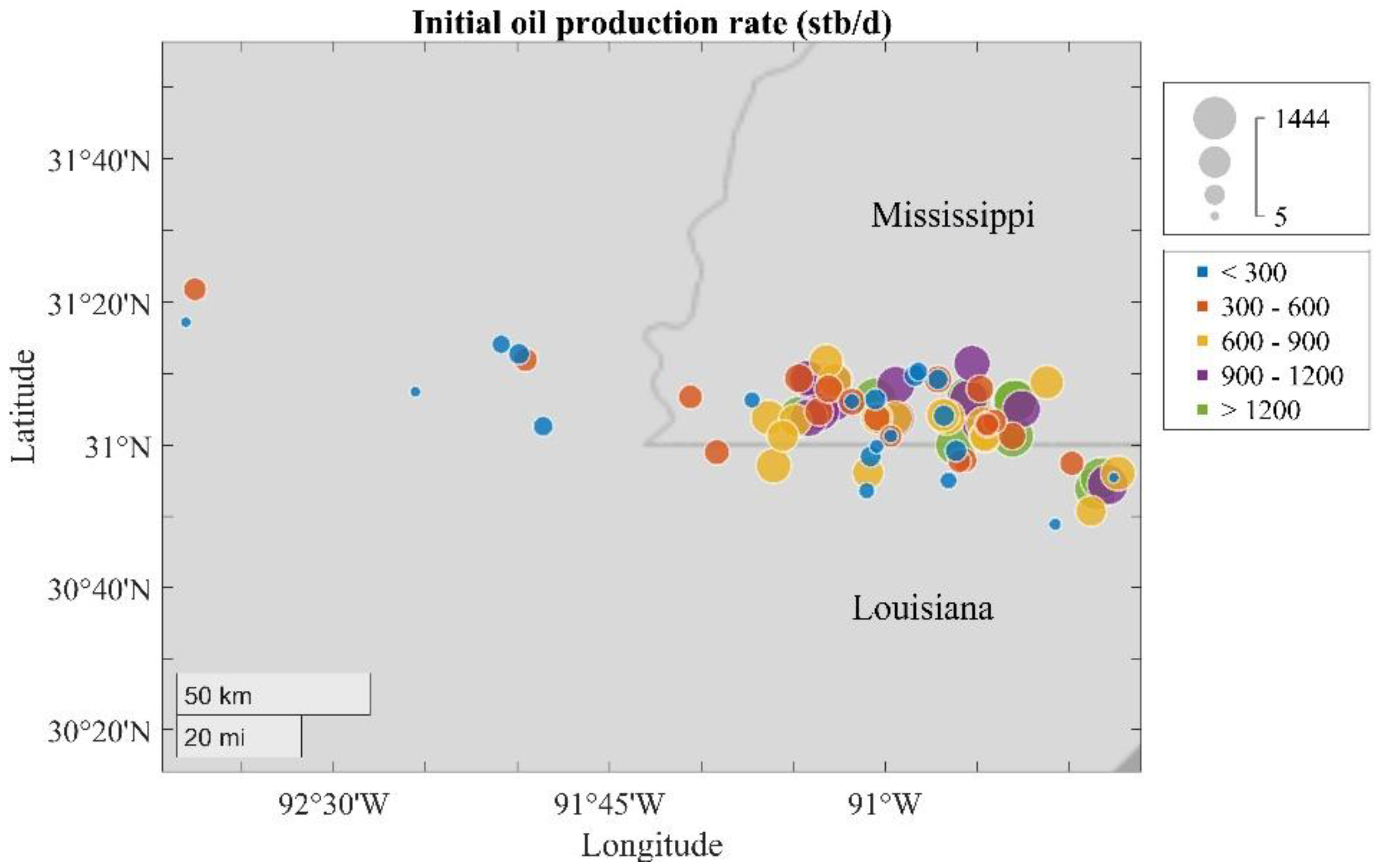
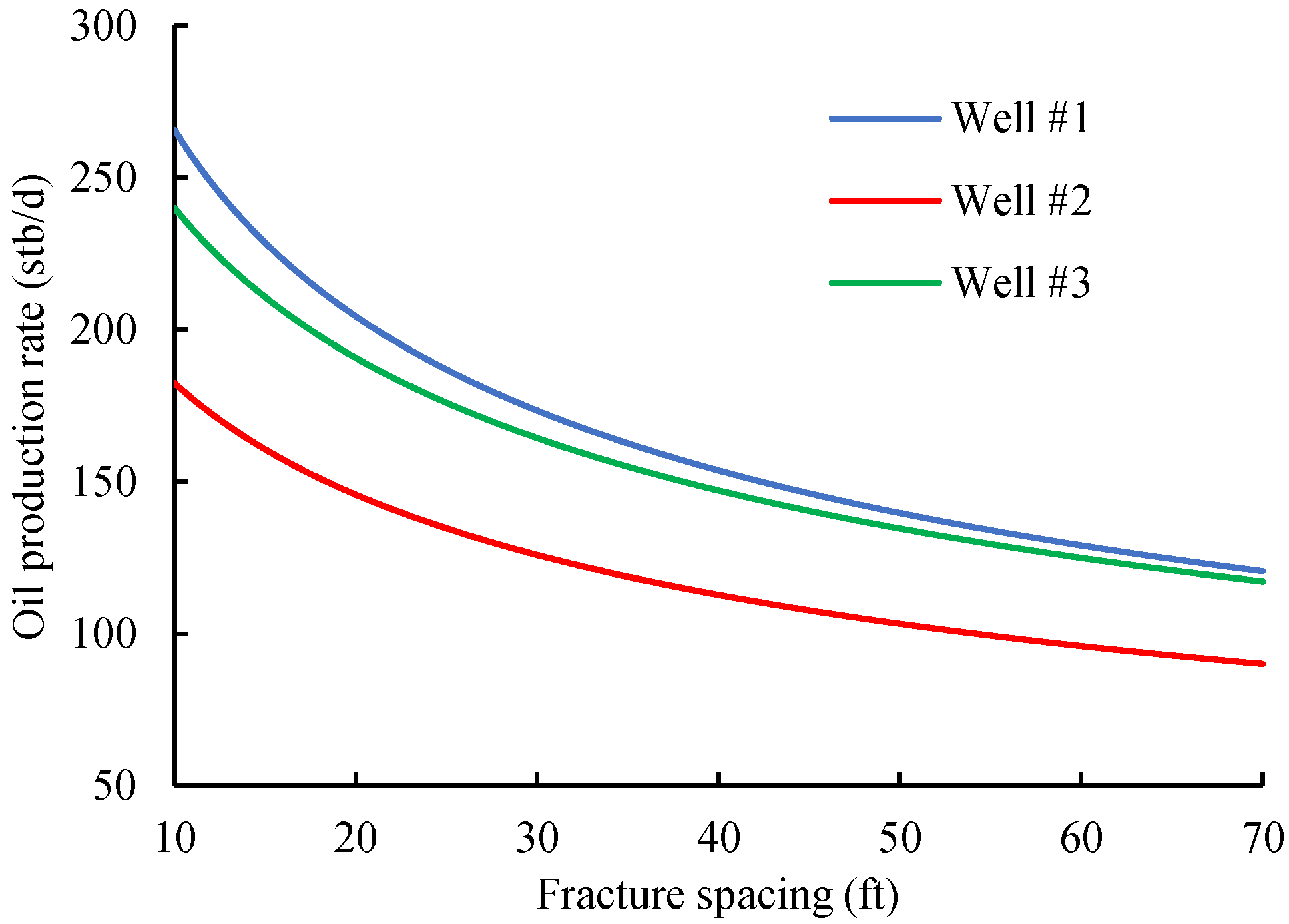
4. Field Case Studies

The Tuscaloosa Marine Shale (TMS) formation, deposited during the Upper Cretaceous, extends from Louisiana to the southern portion of the Mississippi. Little Creek Field is located in Lincoln and Pike Counties, southwestern Mississippi, on the south rim of the Mississippi Salt Basin. It is within the Upper Cretaceous Mid-Dip Tuscaloosa trend, which occurs updip of the Lower Cretaceous shelf margin. In the Mississippi, production from the Mid-Dip trend extends 150 mi (240 km) to the east-southeast from the Mississippi River in a belt 30 to 60 mi (50–100 km) wide. Reservoir rocks are fine- to medium-grained sublitharenite in the stratigraphic unit of the Lower Tuscaloosa formation in the Late Cretaceous, Cenomanian, deposited in the fluvial meander belt environment. The productive facies are point bars. Rock total porosity is 21% to 27% with 13% to 15% primary, 3% to 4% secondary dissolution, and 5% to 8% microporosity. Core porosity ranges 10% to 35% with an average value of 24%. The core permeability measured with air ranges from 0.1 to 100 md with an average value of 10 md. The initial water saturation is between 40% and 75%, averaging at 55%. The reservoir is composed of Q and Q2 sandstone members at an average depth of 10,770 ft (3283 m) in an area of 6 × 3 mi² (9.7 × 4.8 km²). The productive area is 6200 acres (2510 ha.) The hydrocarbon column height is 100 ft (30.5 m) with oil-water at 10,390 ft (3167 m) subsea. The gross sandstone thickness ranges from 15 to 85 ft (4.6–25.9 m), averaging at 40 ft (12.2 m). The average net sandstone thickness is 30 ft (9.1 m). The original reservoir pressure is 4840 psi (3.3 × 10⁴ kPa) at 10,340 feet (3152 m) subsea. The oil has an API gravity of 39° with a GOR (gas/oil ratio) of 555:1 scf/stb and formation volume factor of 1.32. Oil viscosity is up to 5 cp (5.0 × 10⁻³ Pa·s) at 200 °F (93 °C).

TMS needs to use multifractured horizontal wells to become rejuvenated into a key exploration target for the industry as a leading oil field. Production rate and cumulative production data in May 2018 were gathered from 80 TMS wells in Louisiana and Mississippi. The majority of TMS wells were characterized by transient production behaviors.

Selection of wells for analysis in this study was based on the bubble map of the initial well productivity shown in Figure 4. Wells were selected from the Louisiana side of TMS with analyzable production decline curves. Only wells with initial oil production rates between 300 and 1200 stb/d were selected so wells with severe formation damage could be excluded. Wells with abnormal water cuts and gas-oil ratios were also excluded.

Figure 5 shows the statistical results of slopes of 44 TMS wells that were used to identify RLF. It should be mentioned that 11 TMS wells were not analyzed owing to their abrupt changes in production rate over time. We saw that the slopes of 15 wells were in the range of −0.52 and −0.48. Based on the log–log plot of data from 44 oil wells in the TMS trend, a slope of −0.5 was observed for some wells but not all wells. The correlation coefficient between the initial production rate and the slope was −0.076, which meant that there was no linear correlation.

Figure 6 shows the log–log diagnostic plot of production rate data from Well #1. This well was drilled and completed with a horizontal length of 9102 ft and a 29-stage fracturing operation. Four perforation clusters were made in each stage, giving an average cluster spacing of 69 ft. Time data up to five months showed a −0.51 slope (very close to −0.5), indicating RLF. Late time production rate data versus material balance time followed a linear trend line with a slope of −0.78. A plot of the same production data versus actual production time formed a linear trend line with a slope of −1.03, indicating typical behavior for the boundary-dominated flow.

Figure 7 shows the log–log diagnostic plot of production rate data from Well #2. This well was 11,300 ft deep with an effective lateral length of 4791 ft. Time data up to five months showed a −0.51 slope (very close to −0.5), indicating RLF. RLF ended at a production rate of about 226 stb/d. Late time production rate data versus material balance time followed a linear trend line with a slope of −0.76. A plot of the same production data versus actual time formed a linear trend line with a slope of −1.03, indicating typical behavior for BDF.

Figure 8 demonstrates the log–log diagnostic plot of production rate data for Well #3. This well was drilled and completed with a 6099 ft lateral length and a 24-stage fracturing operation. Time data up to four months showed a −0.50 slope, indicating RLF. Late time production rate data versus material balance time followed a linear trend line with a slope of −0.72. A plot of the same production data versus actual production time formed a linear trend line with a slope of −1.00. The pseudosteady production rate was about 126 stb/d at the beginning of the BDF.

Table 1. Reservoir and well completion data.

Parameters	Well #1	Well #2	Well #3
Matrix permeability	0.000105 md	0.000105 md	0.000112 md
Porosity	0.08	0.08	0.08
Slope of square root time curve	0.00032	0.00042	0.00035
Pay zone thickness	135 ft	135 ft	135 ft
Reservoir pressure	6127 psia	5876 psia	6367 psia
Wellbore pressure	4124 psi	3955 psi	4286 psi
Oil formation volume factor	1.3 rb/stb	1.3 rb/stb	1.3 rb/stb
Oil viscosity	0.5 cp	0.5 cp	0.5 cp
Total compressibility	0.00001 psi−1	0.00001 psi−1	0.00001 psi−1
Number of perforation clusters	116	76	96
Perforation cluster spacing	69 ft	63 ft	58 ft
Hydraulic fracture half-length	315 ft	379 ft	321 ft
Volume of proppant	19,090,000 lbs	15,050,000 lbs	161,110,000 lbs
Time at the end of linear flow	180 d	150 d	120 d

presents a summary of the estimated reservoir and well completion/fracture data for these three wells. It was assumed that fractures were created from all perf clusters for simplicity. The fracture height used in this analysis was discounted from the pay zone thickness to the net pay. It should be mentioned that typical values were taken from the area for all wells because there was a lack of fracture job data. The formation pressure gradient and the bottom hole pressure gradient were assumed to be 0.52 and 0.35 psia/ft, respectively. Matrix permeability was estimated using the following equation [33,34]:

$$k_m=\frac{\varphi u_o{c}_t}{t_{ehs}}{\left(\frac{S_f}{2\times 0.159}\right)}^2,$$

(10)

where t_ehs is the time at the end of the half slope in days.

The average fracture spacing can be estimated using the following equations [33,34]:

$$x_f=\sqrt{\eta }\frac{31.277{\mu }_o{B}_o}{n_f{k}_m{h}_f\left(p_e-p_w\right)}\frac{1}{m},$$

(11)

$$\eta =\frac{k_m}{\varphi {\mu }_o{c}_t},$$

(12)

where η is the diffusivity in md∙psia∙cp⁻¹, m is the slope of the inverse of production rate versus $\sqrt{t}$ in day^1/2∙stb⁻¹, and c_t is the total compressibility in psi⁻¹.

Figure 9 illustrates the calculated well productivity curve generated using the data as input to Equation (7). It showed that the model-predicted well production rate at the beginning of BDF was 121 stb/d (at S_f =69 ft), which was 0.83% higher than the observed value of 120 stb/d. The production rate at the beginning of BDF of Well #1 for S_f = 15 ft was 89% higher than that for S_f = 69 ft. This was explained by Wattenbarger’s solution for the initial production rate [34]. It demonstrated that well production rate in the RLF period was proportional to the total fracture surface area. For a given horizontal wellbore length, the total fracture surface is dependent on the number of hydraulic fractures. Therefore, decreasing fracture spacing can increase production rate if the fracture half-length is held constant. Similarly, this indicated that the model-calculated well production rate at the beginning of BDF of Well #2 was 94 stb/d (at S_f = 63 ft), which was 2.08% lower than the observed value of 96 stb/d. When the fracture spacing was reduced to 15 ft, the production rate at the beginning of BDF should be 71% higher than that the original one, assuming no other complex factors were missing in the model development. Of course, the decrease in perf cluster spacing may have less than ideal impacts on well productivity as a result of other complex factors that were not considered in the model development.

Figure 10 demonstrates the diagnostic plot of production rate data for Well #4. Early production data showed a trend with a slope of −0.57, which was between −0.5 and −1, not indicating RLF. This could be due to the existence of natural fractures or the interference of hydraulic fractures. Figure 11 and Figure 12 present the diagnostic plot of production rate data for Well #5 and Well #6, respectively. Early production data showed trends with slope values of −0.58 and −0.62, respectively, not indicating RLF. This could be due to the existence of natural fractures or the interference of hydraulic fractures. The bubble map in Figure 4 was compared with geological maps for natural fracture/shale quality identification. A further examination of locations of Wells #4, #5, and #6 confirmed that these wells were drilled in an area where multiple natural fractures were found. It was generally believed that not all the hydraulic fractures were equal in length, owing to heterogeneity within the reservoir or stress shadow. Ambrose et al. [33] indicated fracture interference had a great effect on the performance of a well. They demonstrated that fracture interference tended to increase the cumulative production. However, the higher the heterogeneity, the less the recovery factor. It was therefore not recommended to reduce fracture spacing for these wells or wells in the areas.

5. Conclusions

In summary, the performances of multifracture horizontal wells (MFHW) in shale oil fields in different regions of the world are mixed. This is believed partially because of the lack of optimization of well completion parameters, especially fracture spacing. Optimization of such spacing is generally recognized as one of the most important steps in enabling economic horizontal wells and requires a lot of attention. A data-driven workflow approach is presented in this study for optimizing fracture spacing of MFHW in shale oil reservoirs. Fracture spacing should be as short as possible unless "interference" occurs, and this "interference" can be found from the pressure transient analysis. If the interference does not happen in initial stages, well productivity can be improved by shortening the fracture spacing. The following conclusions were drawn from this study.

• This workflow procedure has the advantage of using an analytical well productivity model driven by real production data, making it a practical approach to optimize MFHW in shale oil reservoirs.
• This workflow procedure employs a closed-form analytical solution and provides a transparent approach to the identification of important fracturing parameters affecting well productivity.
• This workflow procedure uses transient pressure or production data to identify fracture interference. This offers a reliable and cost-effective means for assessing well production potential in terms of optimizing fracture spacing in the MFHW.
• Results of a field case study indicated that three wells were drilled and completed with fracture spacing values that were short enough to effectively drain the stimulated reservoir volume (SRV), while the other three wells were drilled and completed with fracture spacings that could be shortened to significantly improve well productivity.

References

1. Rafiee, M.; Soliman, M.Y.; Pirayesh, E. Hydraulic fracturing design and optimization: A modification to zipper frac. In Proceedings of the SPE Easter Regional Meeting, San Antonio, TX, USA, 8–10 October 2012. [Google Scholar]
2. Ren, J.; Guo, P. A general analytical method for transient flow rate with the stress-sensitive effect. J. Hydrol. 2018, 565, 262–275. [Google Scholar] [CrossRef]
3. Xue, L.; Chen, X.; Wang, L. Pressure transient analysis for fluid flow through horizontal fractures in shallow organic compound reservoir of hydrogen and carbon. Int. J. Hydrogen Energy 2019, 44, 5245–5253. [Google Scholar] [CrossRef]
4. Bajwa, A.I.; Blunt, M.J. Early-time 1D analysis of shale-oil and-gas flow. SPE J. 2016, 21, 1254–1262. [Google Scholar] [CrossRef]
5. Abbasi, M.; Madani, M.; Sharifi, M.; Kazemi, A. Fluid flow in fractured reservoirs: Exact analytical solution for transient dual porosity model with variable rock matrix block size. J. Pet. Sci. Eng. 2018, 164, 571–583. [Google Scholar] [CrossRef]
6. Sesetty, V.; Ghassemi, A. A numerical study of sequential and simultaneous hydraulic fracturing in single and multi-lateral horizontal wells. J. Pet. Sci. Eng. 2015, 132, 65–76. [Google Scholar] [CrossRef]
7. Li, J.; Xiao, W.; Hao, G.; Dong, S.; Hua, W.; Li, X. Comparison of different hydraulic fracturing scenarios in horizontal wells using XFEM based on the cohesive zone method. Energies 2019, 12, 1232. [Google Scholar] [CrossRef]
8. Du, X.; Nydal, O.J. Flow models and numerical schemes for single/two-phase transient flow in one dimension. Appl. Math. Model. 2017, 42, 145–160. [Google Scholar] [CrossRef] [Green Version]
9. Yu, W.; Xu, Y.; Weijermars, R.; Wu, K.; Sepehrnoori, K. Impact of well interference on shale oil production performance: A numerical model for analyzing pressure response of fracture hits with complex cemeteries. In Proceedings of the SPE Hydraulic Fracturing Technology Conference and Exhibition, The Woodlands, TX, USA, 24–26 January 2017. [Google Scholar]
10. He, Y.; Cheng, S.; Rui, Z.; Qin, J.; Fu, L.; Shi, J.; Wang, Y.; Li, D.; Patil, S.; Yu, H.; Lu, J. An improved rate-transient analysis model of multi-fractured horizontal wells with non-uniform hydraulic fracture properties. Energies 2018, 11, 393. [Google Scholar] [CrossRef]
11. Sun, H.; Zhou, D.; Chawathé, A.; Du, M. Quantifying shale oil production mechanisms by integrating a Delaware basin well data from fracturing to production. In Proceedings of the Unconventional Resources Technology Conference, San Antonio, TX, USA, 1–3 August 2016. [Google Scholar]
12. Orangi, A.; Nagarajan, N.R.; Honarpour, M.M.; Rosenzweig, J.J. Unconventional shale oil and gas-condensate reservoir production, impact of rock, fluid, and hydraulic fractures. In Proceedings of the SPE Hydraulic Fracturing Technology Conference and Exhibition, The Woodlands, TX, USA, 24–26 January 2011. [Google Scholar]
13. Guo, B.; Yu, X.; Khoshgahdam, M. A simple analytical model for predicting productivity of multifractured horizontal wells. SPE Reserv. Eval. Eng. 2009, 12, 879–885. [Google Scholar] [CrossRef]
14. Zhang, C.; Wang, P.; Guo, B.; Song, G. Analytical modeling of productivity of multi-fractured shale gas wells under pseudo-steady flow conditions. Energy Sci. Eng. 2018, 6, 819–827. [Google Scholar] [CrossRef]
15. Li, G.; Guo, B.; Li, J.; Wang, M. A mathematical model for predicting long-term productivity of modern multifractured shale gas/oil wells. SPE Drill. Complet. 2019, 34. [Google Scholar] [CrossRef]
16. Guo, B.; Liu, X.; Tan, X. Petroleum Production Engineering, 2nd ed.; Elsevier: Cambridge, MA, USA, 2017; pp. 432–489. ISBN 978-0-12-809374-0. [Google Scholar]
17. Potapenko, D.I.; Williams, R.D.; Desroches, J.; Enkababian, P.; Theuveny, B.; Willberg, D.M.; Conort, G. Securing long-term well productivity of horizontal wells through optimization of postfracturing operations. In Proceedings of the SPE Annual Technical Conference and Exhibition, San Antonio, TX, USA, 9–11 October 2017. [Google Scholar]
18. Feng, F.; Wang, X.; Guo, B.; Ai, C. Mathematical model of fracture complexity indicator in multistage hydraulic fracturing. J. Nat. Gas Sci. Eng. 2017, 38, 39–49. [Google Scholar] [CrossRef]
19. Zhang, Q.; Wang, X.; Wang, D.; Zeng, J.; Zeng, F.; Zhang, L. Pressure transient analysis for vertical fractured wells with fishbone fracture patterns. J. Nat. Gas Sci. Eng. 2018, 52, 187–201. [Google Scholar] [CrossRef]
20. Li, D.; Zha, W.; Liu, S.; Wang, L.; Lu, D. Pressure transient analysis of low permeability reservoir with pseudo threshold pressure gradient. J. Pet. Sci. Eng. 2016, 147, 308–316. [Google Scholar] [CrossRef]
21. Wu, Z.; Cui, C.; Lv, G.; Bing, S.; Cao, G. A multi-linear transient pressure model for multistage fractured horizontal well in tight oil reservoirs with considering threshold pressure gradient and stress sensitivity. J. Pet. Sci. Eng. 2019, 172, 839–854. [Google Scholar] [CrossRef]
22. Fekete, F.A.S.T. Well Test User Manual; Fekete Associates, Inc.: Calgary, AB, Canada, 2003. [Google Scholar]
23. E-Production Services, Inc. PanSystem User Manual; E-Production Services, Inc.: Edinburgh, UK, 2004. [Google Scholar]
24. Shan, L.; Guo, B.; Weng, D.; Liu, Z.; Chu, H. Posteriori assessment of fracture propagation in refractured vertical oil wells by pressure transient analysis. J. Pet. Sci. Eng. 2018, 168, 8–16. [Google Scholar] [CrossRef]
25. Pang, W.; Wu, Q.; He, Y. Production analysis of one shale gas reservoir in China. In Proceedings of the SPE Annual Technical Conference and Exhibition, Houston, TX, USA, 28–30 September 2015. [Google Scholar]
26. He, Y.; Cheng, S.; Li, S.; Huang, Y.; Qin, J.; Hu, L.; Yu, H. A semianalytical methodology to diagnose the locations of underperforming hydraulic fractures through pressure-transient analysis in tight gas reservoir. SPE J. 2017, 22, 924–939. [Google Scholar] [CrossRef]
27. Cinco, L.H.; Samaniego, V.F. Transient Pressure Analysis for Fractured Wells. J. Pet. Technol. 1981, 33, 1749–1766. [Google Scholar] [CrossRef]
28. Gringarten, A.C.; Ramey, H.J.; Raghavan, R. Applied pressure analysis for fractured wells. J. Pet. Technol. 1975, 27, 887–892. [Google Scholar] [CrossRef]
29. Cinco, L.H.; Samaniego, V.; Dominguez, A. Transient pressure behavior for a well with a finite-conductivity vertical fracture. Soc. Pet. Eng. J. 1978, 18, 253–264. [Google Scholar] [CrossRef]
30. Uzun, I.; Kurtoglu, B.; Kazemi, H. Multiphase rate-transient analysis in unconventional reservoirs: Theory and application. SPE Reserv. Eval. Eng. 2016, 19, 553–566. [Google Scholar] [CrossRef]
31. Yang, C.; Sharma, V.K.; Datta-Gupta, A.; King, M.J. Novel approach for production transient analysis of shale reservoirs using the drainage volume derivative. J. Pet. Sci. Eng. 2017, 159, 8–24. [Google Scholar] [CrossRef]
32. Marsden, J.; Kostyleva, I.; Fassihi, M.R.; Gringarten, A.C. A conceptual shale gas model validated by pressure and rate data from the Haynesville shale. In Proceedings of the SPE Annual Technical Conference and Exhibition, San Antonio, TX, USA, 9–11 October 2017. [Google Scholar]
33. Ambrose, R.J.; Clarkson, C.R.; Youngblood, J.E.; Adams, R.; Nguyen, P.D.; Nobakht, M.; Biseda, B. Life-cycle decline curve estimation for tight/shale reservoirs. In Proceedings of the SPE Hydraulic Fracturing Technology Conference, The Woodlands, TX, USA, 24–26 January 2011. [Google Scholar] [CrossRef]
34. Wattenbarger, R.A.; El-Banbi, A.H.; Villegas, M.E.; Maggard, J.B. Production analysis of linear flow into fractured tight gas wells. In Proceedings of the SPE Rocky Mountain Regional/Low-Permeability Reservoirs Symposium, Denver, CO, USA, 5–8 April 1998. [Google Scholar] [CrossRef]
Figure 1. Twelve hydraulic fractures developed from 12 perforation clusters in three stages of fracturing.
Energies 12 01973 g001
Figure 2. Diagnostic plot of pressure transient data for flow regime identification.
Energies 12 01973 g002
Figure 3. Diagnostic plot of rate transient data for flow regime identification.
Energies 12 01973 g003
Figure 4. Bubble map of the initial well productivity of Tuscaloosa Marine Shale (TMS) wells.
Energies 12 01973 g004
Figure 5. Statistical results of slopes used to identify reservoir linear flow (RLF).
Energies 12 01973 g005
Figure 6. Plot of production rate data for Well #1.
Energies 12 01973 g006
Figure 7. Plot of production rate data for Well #2.
Energies 12 01973 g007
Figure 8. Plot of production rate data for Well #3.
Energies 12 01973 g008
Figure 9. Model-calculated productivity for TMS wells.
Energies 12 01973 g009
Figure 10. Plot of production rate data for Well #4.
Energies 12 01973 g010
Figure 11. Plot of production rate data for Well #5.
Energies 12 01973 g011
Figure 12. Plot of production rate data for Well #6.
Energies 12 01973 g012