The Optimized Energy Saving of a Refrigerating Chamber


Abstract
1. Introduction
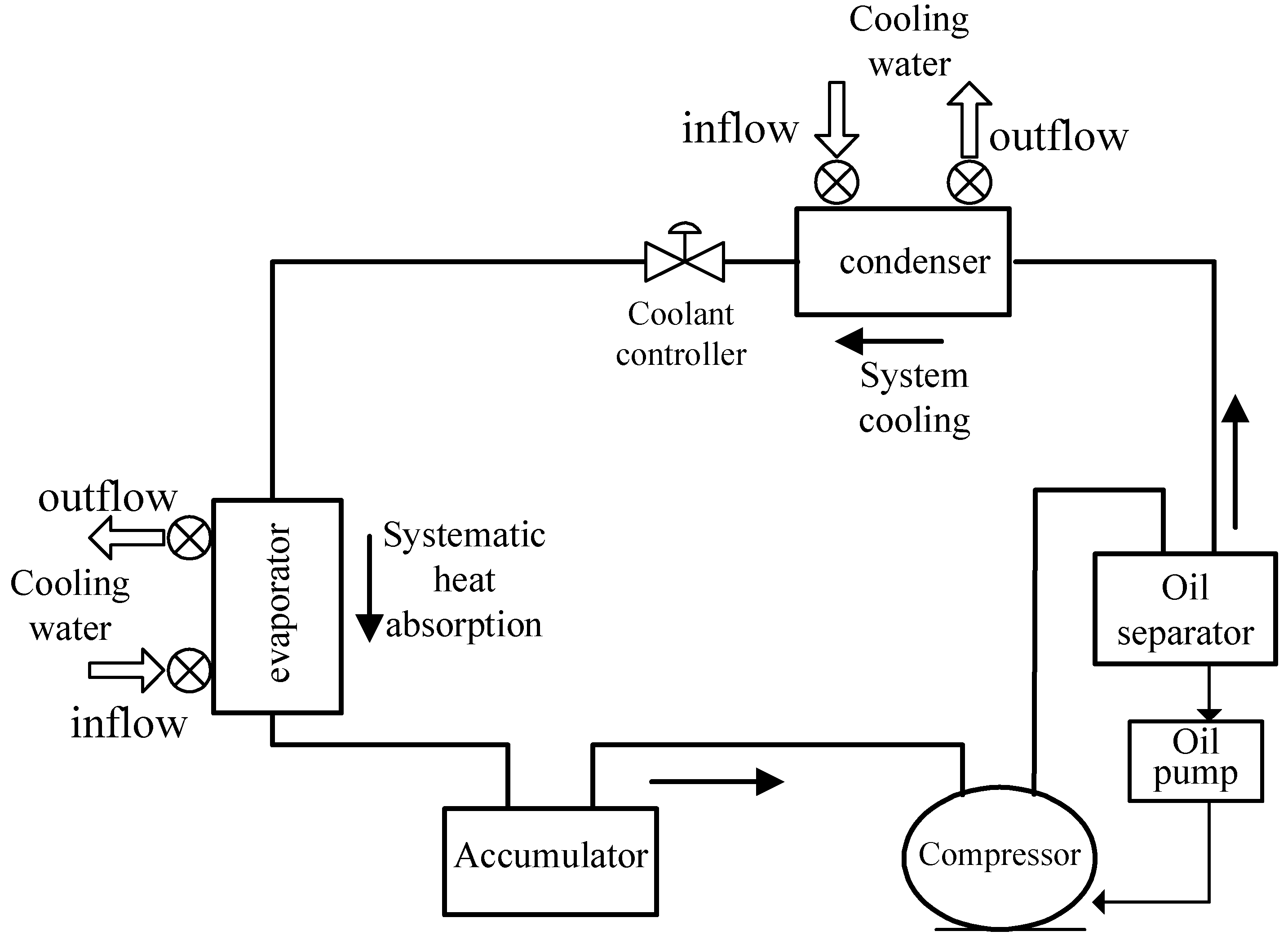
2. System Structure
3. The Control Strategy for the Energy Saving of a Refrigerating Chamber
3.1. Proteome Reorganization
3.2. The Control Strategy of Refrigerating Chambers
- Temperature limitation of refrigerating chamber,where is the temperature of refrigerating chambers, is the preset floor temperature of refrigerating chambers, and is the preset ceiling temperature of refrigerating chambers;
- Shortest turn-off time limitation of electromagnetic valve.
3.3. Implementation of BPA
4. Case Study
4.1. The Control Strategy Analysis of the Refrigerating Chamber
4.2. The Energy-Saving Analysis of the Refrigerating Chamber
- According to the comparison among Table 2, Table 4 and Table 5, when the No. 9 refrigerating chamber was in time stages 5, 6, 7, and 20, and the No. 10 refrigerating chamber was in time stage 20, the status of the electromagnetic valve was changed from on to off by the energy control strategy, as the temperature met the limitation set in the time stages.
- According to the comparison between Table 3 and Table 6, the total load was 183 kW in time stage 5, the total power consumption of the system was 114.4 kW, and the COP value was 1.6. After the energy conservation strategy was performed in the same time stage, the total load decreased to 168 kW, the total power consumption of the system was 70 kW, and the COP value was 2.4.
- When the No. 9 refrigerating chamber was in time stages 6, 7, and 20, and the No. 10 refrigerating chamber was in time stage 20, the electromagnetic valve was turned off by the control strategy for the same reason, and the #2 compressor was shut down. This action not only increased the COP value in these stages, it also reduced the total power consumption of the system.
- As shown in Figure 10, in time stages 5, 6, 7, and 20, as the temperatures of the No. 9 and No. 10 refrigerating chambers met the electromagnetic valve off condition, the electromagnetic valve was turned off, and the refrigerating chamber load decreased; thus, the total system load decreased.
4.3. BPA Performance Test
4.4. Test for BPA Considering Switching Loss
5. Conclusions
Author Contributions
Funding
Acknowledgments
Conflicts of Interest
References
- Althouse, A.D.; Turnquist, C.H.; Bracciano, A.F.; Bracciano, D.C.; Bracciano, G.M. Modern Refrigeration and Air Conditioning, 20th ed.; The Goodheart-Willcox Co. Inc.: Tinley Park, IL, USA, 2017. [Google Scholar]
- Babiloni, A.M.; Esbrí, A.N.; Cervera, A.B.; Moles, F.; Verdu, G. Commercial refrigeration—An overview of current status. Int. J. Refrig. 2015, 57, 186–196. [Google Scholar] [CrossRef]
- Chen, M.C. Refrigeration Engineering (II); Chang Nuo Information Books: Taipei, Taiwan, 1999; pp. 3–4. [Google Scholar]
- Food and Agriculture Organization of the United Nations. Design and Operation of Cold Stores in Developing Countries; International Institute Refrigeration: Paris, France, 1984. [Google Scholar]
- Son, C.H. A study on the prediction of the future demand for cold-storage facilities in South Korea. Int. J. Refrig. 2012, 35, 2078–2084. [Google Scholar] [CrossRef]
- Salazar, M.; Méndez, F. PID control for a single-stage transcritical CO2 refrigeration cycle. Appl. Therm. Eng. 2014, 67, 429–438. [Google Scholar] [CrossRef]
- Li, B.; Otten, R.; Chandan, V.; Mohs, W.F.; Alleyne, A.G. Optimal on–off control of refrigerated transport systems. Control Eng. Pract. 2010, 18, 1406–1417. [Google Scholar] [CrossRef]
- Yan, H.; Xia, Y.; Deng, S. Adaptive control for degree of refrigerant superheat in a direct expansion air conditioning system under variable speed operation. Energy Procedia 2019, 158, 2182–2187. [Google Scholar] [CrossRef]
- Huang, Y.; Khajepour, A.; Bagheri, F.; Bahrami, M. Optimal energy-efficient predictive controllers in automotive air-conditioning/refrigeration systems. Appl. Energy 2016, 184, 605–618. [Google Scholar] [CrossRef]
- Powell, K.M.; Cole, W.J.; Ekarika, U.F.; Edgar, T.F. Optimal chiller loading in a district cooling system with thermal energy storage. Energy 2013, 50, 445–453. [Google Scholar] [CrossRef]
- Chua, K.J.; Chou, S.K.; Yang, W.M.; Yan, J. Achieving better energy-efficient air conditioning—A review of technologies and strategies. Appl. Energy 2013, 104, 87–104. [Google Scholar] [CrossRef]
- Cutillas, C.G.; Ramírez, J.R.; Miralles, ML. Optimum Design and Operation of an HVAC Cooling Tower for Energy and Water Conservation. Energies 2017, 10, 299. [Google Scholar] [CrossRef]
- Sepehr, S.; Ali, S. Thermo-economic optimization of an ice thermal energy storage system for air-conditioning applications. Energy Build. 2013, 60, 100–109. [Google Scholar]
- Jara, P.B.T.; Rivera, J.J.A.; Merino, C.E.B.; Silva, E.V.; Farfán, G.A. Thermal behavior of a refrigerated vehicle: Process simulation. Int. J. Refrig. 2019, 100, 124–130. [Google Scholar] [CrossRef]
- Hoang, M.H.; Laguerre, O.; Moureh, J.; Flick, D. Heat transfer modelling in a ventilated cavity loaded with food product: Application to a refrigerated vehicle. J. Food Eng. 2012, 113, 389–398. [Google Scholar] [CrossRef]
- Bejarano, G.; Rodríguez, D.; Alfaya, J.A.; Gil, J.D.; Ortega, M.G. Optimization and Cascade Robust Temperature Control of a Refrigerated Chamber. IFAC-Pap. 2018, 51, 110–115. [Google Scholar] [CrossRef]
- Oludaisi, A.; Tamba, J.; Rotimi, S.; Zhongie, H. Minimizing energy consumption in refrigerated vehicles through alternative external wall. Renew. Sustain. Energy Rev. 2017, 67, 89–93. [Google Scholar]
- Giráldez, H.; Pérez Segarra, C.D.; Oliet, C.; Oliva, A. Heat and moisture insulation by means of air curtains: Application to refrigerated chambers. Int. J. Refrig. 2016, 68, 1–14. [Google Scholar] [CrossRef]
- Wan, Y.; Wang, M.; Ye, Z.; Lai, X. A feature selection method based on modified binary coded ant colony optimization algorithm. Appl. Soft Comput. 2016, 49, 248–258. [Google Scholar] [CrossRef]
- Menhas, M.H.; Wang, L.; Fei, M.; Pan, H. Comparative performance analysis of various binary coded PSO algorithms in multivariable PID controller design. Expert Syst. Appl. 2012, 39, 4390–4401. [Google Scholar] [CrossRef]
- Sigov, A.; Baranyuk, V.; Nechaev, V.; Smirnova, O.; Melikhov, A. Approach for Forming the Bionic Ontology. Procedia Comput. Sci. 2017, 103, 495–498. [Google Scholar] [CrossRef]
- Yu, F.W.; Chan, K.T. Advanced control of heat rejection airflow for improving the coefficient of performance of air-cooled chillers. Appl. Therm. Eng. 2006, 26, 97–110. [Google Scholar] [CrossRef]
- Chen, H.J.; Wang, D.W.P.; Chen, S.L. Optimization of an ice-storage air conditioning system using dynamic programming method. Appl. Therm. Eng. 2005, 25, 461–472. [Google Scholar] [CrossRef]
- Chang, Y.C.; Lin, F.A.; Lin, C.H. Optimal chiller sequencing by branch and bound method for saving energy. Energy Convers. Manag. 2005, 46, 2158–2172. [Google Scholar] [CrossRef]
- Muller, F.L.; Lustgarten, M.S.; Jang, Y.; Richardson, A.; Van Remmen, H. Trends in oxidative aging theories. Free Radicbiol. 2007, 43, 477–503. [Google Scholar] [CrossRef] [PubMed]
- Ray, P.D.; Huang, B.W.; Tsuji, Y. Reactive oxygen species (ROS) homeostasis and redox regulation in cellular signaling. Cell Signal 2012, 24, 981–990. [Google Scholar] [CrossRef]


| Item | Strategic Objective | Description |
|---|---|---|
| 1 | Optimum refrigerant recirculating status | (1) The electromagnetic valve of the refrigerating chamber is turned off before the upper or lower temperature limit is exceeded. As the load of the refrigeration cycle system decreases, the power input will decrease. |
| (2) As the refrigerant circulation decreases, the load of the compressor decreases, such that the power input work decreases, and the high/low pressure of the system is influenced. The expansion valve opening is increased, while the refrigerant flow decreases; thus, as the high pressure drops and the low pressure remains, the power input of the compressor decreases. | ||
| 2 | Full load of compressor | (1) When the status of the reorganization valve in the refrigerating chamber is on, the refrigerant enters the refrigerating chamber via the expansion valve to absorb the heat energy in the chamber, while the overheated refrigerant, which absorbed the heat energy, returns to the low-pressure end of the compressor. Therefore, the more electromagnetic valves are turned on, the more overheated refrigerant returns to the low-pressure suction end of the compressor, and the refrigeration load of the refrigeration cycle system increases. The electromagnetic valve of the refrigerating chamber is turned on before the upper or lower temperature limit is exceeded, and the running compressor is in the full-load status. |
| (2) On the other hand, the electromagnetic valve of a refrigerating chamber is turned off before the upper or lower temperature limit is exceeded, and the total load of the refrigeration cycle system is reduced, which switches off the compressor under low load, while the running compressor remains in full-load conditions at any time. |
| Time Stage | Chamber | 1 | 2 | 3 | 4 | 5 | 6 | 7 | 8 | 9 | 10 | Total Load | |
|---|---|---|---|---|---|---|---|---|---|---|---|---|---|
| Time | |||||||||||||
| 1 | 11:00–11:05 a.m. | 30.0 | 33.0 | 34.5 | 35.0 | 34.0 | 0.0 | 0.0 | 0.0 | 0.0 | 0.0 | 166.5 | |
| 2 | 11:05–11:10 a.m. | 30.0 | 33.0 | 34.5 | 35.0 | 34.0 | 0.0 | 0.0 | 0.0 | 0.0 | 0.0 | 166.5 | |
| 3 | 11:10–11:15 a.m. | 30.0 | 33.0 | 34.5 | 35.0 | 34.0 | 0.0 | 0.0 | 0.0 | 0.0 | 0.0 | 166.5 | |
| 4 | 11:15–11:20 a.m. | 25.0 | 34.0 | 34.5 | 35.0 | 34.0 | 0.0 | 0.0 | 0.0 | 0.0 | 0.0 | 162.5 | |
| 5 | 11:20–11:25 a.m. | 25.0 | 34.0 | 30.0 | 35.0 | 34.0 | 0.0 | 0.0 | 10.0 | 25.0 | 0.0 | 193.0 | |
| 6 | 11:25–11:30 a.m. | 32.0 | 34.0 | 30.0 | 35.0 | 34.0 | 0.0 | 0.0 | 10.0 | 25.0 | 0.0 | 200.0 | |
| 7 | 11:30–11:35 a.m. | 33.0 | 35.0 | 30.0 | 35.0 | 34.0 | 0.0 | 0.0 | 5.0 | 25.0 | 0.0 | 197.0 | |
| 8 | 11:35–11:40 a.m. | 33.0 | 35.0 | 34.5 | 35.0 | 34.0 | 32.0 | 33.0 | 24.0 | 25.0 | 0.0 | 285.5 | |
| 9 | 11:40–11:45 a.m. | 33.0 | 34.0 | 34.5 | 35.0 | 34.0 | 32.0 | 33.0 | 24.0 | 25.0 | 0.0 | 284.5 | |
| 10 | 11:45–11:50 a.m. | 34.0 | 34.0 | 34.5 | 35.0 | 34.0 | 32.0 | 33.0 | 24.0 | 25.0 | 15.0 | 300.5 | |
| 11 | 11:50–11:55 a.m. | 34.0 | 26.0 | 34.5 | 35.0 | 34.0 | 32.0 | 33.0 | 24.0 | 25.0 | 15.0 | 292.5 | |
| 12 | 11:55 a.m.–12:00 p.m. | 34.0 | 24.0 | 34.5 | 27.0 | 29.0 | 32.0 | 33.0 | 24.0 | 27.0 | 15.0 | 279.5 | |
| 13 | 12:00–12:05 p.m. | 34.0 | 24.0 | 25.0 | 27.0 | 29.0 | 32.0 | 33.0 | 24.0 | 27.0 | 15.0 | 270.0 | |
| 14 | 12:05–12:10 p.m. | 34.0 | 24.0 | 25.0 | 27.0 | 29.0 | 32.0 | 33.0 | 24.0 | 27.0 | 15.0 | 270.0 | |
| 15 | 12:10–12:15 p.m. | 35.0 | 24.0 | 25.0 | 27.0 | 29.0 | 32.0 | 33.0 | 24.0 | 27.0 | 15.0 | 271.0 | |
| 16 | 12:15–12:20 p.m. | 35.0 | 15.0 | 25.0 | 27.0 | 29.0 | 32.0 | 19.0 | 24.0 | 27.0 | 15.0 | 248.0 | |
| 17 | 12:20–12:25 p.m. | 25.0 | 15.0 | 25.0 | 27.0 | 29.0 | 32.0 | 19.0 | 24.0 | 27.0 | 15.0 | 238.0 | |
| 18 | 12:25–12:30 p.m. | 23.0 | 15.0 | 25.0 | 14.0 | 29.0 | 32.0 | 19.0 | 24.0 | 27.0 | 15.0 | 223.0 | |
| 19 | 12:30–12:35 p.m. | 22.0 | 15.0 | 25.0 | 14.0 | 29.0 | 32.0 | 19.0 | 24.0 | 27.0 | 15.0 | 222.0 | |
| 20 | 12:35–12:40 p.m. | 21.0 | 15.0 | 0.0 | 14.0 | 29.0 | 23.0 | 19.0 | 31.0 | 27.0 | 15.0 | 194.0 | |
| 21 | 12:40–12:45 p.m. | 10.0 | 22.0 | 0.0 | 14.0 | 17.0 | 23.0 | 19.0 | 31.0 | 0.0 | 15.0 | 151.0 | |
| 22 | 12:45–12:50 p.m. | 10.0 | 22.0 | 0.0 | 14.0 | 17.0 | 23.0 | 19.0 | 31.0 | 0.0 | 15.0 | 151.0 | |
| 23 | 12:50–12:55 p.m. | 10.0 | 22.0 | 0.0 | 14.0 | 17.0 | 23.0 | 19.0 | 31.0 | 0.0 | 25.0 | 161.0 | |
| 24 | 12:55–1:00 p.m. | 10.0 | 22.0 | 0.0 | 14.0 | 17.0 | 23.0 | 19.0 | 31.0 | 0.0 | 25.0 | 161.0 | |
| Time Stage | Classical Control of #1 and #2 Compressor On/Off Status | BPA Control of #1 and #2 Compressor On/Off Status | ||
|---|---|---|---|---|
| #1 Compressor Status | #2 Compressor Status | #1 Compressor Status | #2 Compressor Status | |
| 1 | On | Off | On | Off |
| 2 | On | Off | On | Off |
| 3 | On | Off | On | Off |
| 4 | On | Off | On | Off |
| 5 | On | On | On | Off |
| 6 | On | On | On | Off |
| 7 | On | On | On | Off |
| 8 | On | On | On | On |
| 9 | On | On | On | On |
| 10 | On | On | On | On |
| 11 | On | On | On | On |
| 12 | On | On | On | On |
| 13 | On | On | On | On |
| 14 | On | On | On | On |
| 15 | On | On | On | On |
| 16 | On | On | On | On |
| 17 | On | On | On | On |
| 18 | On | On | On | On |
| 19 | On | On | On | On |
| 20 | On | On | On | Off |
| 21 | On | Off | On | Off |
| 22 | On | Off | On | Off |
| 23 | On | Off | On | Off |
| 24 | On | Off | On | Off |
| Time Stage | Chamber | 1 | 2 | 3 | 4 | 5 | 6 | 7 | 8 | 9 | 10 | Total Load | |
|---|---|---|---|---|---|---|---|---|---|---|---|---|---|
| Time | |||||||||||||
| 1 | 11:00–11:05 a.m. | 30.0 | 33.0 | 34.5 | 35.0 | 34.0 | 0.0 | 0.0 | 0.0 | 0.0 | 0.0 | 166.5 | |
| 2 | 11:05–11:10 a.m. | 30.0 | 33.0 | 34.5 | 35.0 | 34.0 | 0.0 | 0.0 | 0.0 | 0.0 | 0.0 | 166.5 | |
| 3 | 11:10–11:15 a.m. | 30.0 | 33.0 | 34.5 | 35.0 | 34.0 | 0.0 | 0.0 | 0.0 | 0.0 | 0.0 | 166.5 | |
| 4 | 11:15–11:20 a.m. | 25.0 | 34.0 | 34.5 | 35.0 | 34.0 | 0.0 | 0.0 | 0.0 | 0.0 | 0.0 | 162.5 | |
| 5 | 11:20–11:25 a.m. | 25.0 | 34.0 | 30.0 | 35.0 | 34.0 | 0.0 | 0.0 | 0.0 | 0.0 | 0.0 | 168.0 | |
| 6 | 11:25–11:30 a.m. | 32.0 | 34.0 | 30.0 | 35.0 | 34.0 | 0.0 | 0.0 | 0.0 | 0.0 | 0.0 | 175.0 | |
| 7 | 11:30–11:35 a.m. | 33.0 | 35.0 | 30.0 | 35.0 | 34.0 | 0.0 | 0.0 | 0.0 | 0.0 | 0.0 | 172.0 | |
| 8 | 11:35–11:40 a.m. | 33.0 | 35.0 | 34.5 | 35.0 | 34.0 | 32.0 | 33.0 | 24.0 | 25.0 | 0.0 | 285.5 | |
| 9 | 11:40–11:45 a.m. | 33.0 | 34.0 | 34.5 | 35.0 | 34.0 | 32.0 | 33.0 | 24.0 | 25.0 | 0.0 | 284.5 | |
| 10 | 11:45–11:50 a.m. | 34.0 | 34.0 | 34.5 | 35.0 | 34.0 | 32.0 | 33.0 | 24.0 | 25.0 | 15.0 | 300.5 | |
| 11 | 11:50–11:55 a.m. | 34.0 | 26.0 | 34.5 | 35.0 | 34.0 | 32.0 | 33.0 | 24.0 | 25.0 | 15.0 | 292.5 | |
| 12 | 11:55 a.m.–12:00 p.m. | 34.0 | 24.0 | 34.5 | 27.0 | 29.0 | 32.0 | 33.0 | 24.0 | 27.0 | 15.0 | 279.5 | |
| 13 | 12:00–12:05 p.m. | 34.0 | 24.0 | 25.0 | 27.0 | 29.0 | 32.0 | 33.0 | 24.0 | 27.0 | 15.0 | 270.0 | |
| 14 | 12:05–12:10 p.m. | 34.0 | 24.0 | 25.0 | 27.0 | 29.0 | 32.0 | 33.0 | 24.0 | 27.0 | 15.0 | 270.0 | |
| 15 | 12:10–12:15 p.m. | 35.0 | 24.0 | 25.0 | 27.0 | 29.0 | 32.0 | 33.0 | 24.0 | 27.0 | 15.0 | 271.0 | |
| 16 | 12:15–12:20 p.m. | 35.0 | 15.0 | 25.0 | 27.0 | 29.0 | 32.0 | 19.0 | 24.0 | 27.0 | 15.0 | 248.0 | |
| 17 | 12:20–12:25 p.m. | 25.0 | 15.0 | 25.0 | 27.0 | 29.0 | 32.0 | 19.0 | 24.0 | 27.0 | 15.0 | 238.0 | |
| 18 | 12:25–12:30 p.m. | 23.0 | 15.0 | 25.0 | 14.0 | 29.0 | 32.0 | 19.0 | 24.0 | 27.0 | 15.0 | 223.0 | |
| 19 | 12:30–12:35 p.m. | 22.0 | 15.0 | 25.0 | 14.0 | 29.0 | 32.0 | 19.0 | 24.0 | 27.0 | 15.0 | 222.0 | |
| 20 | 12:35–12:40 p.m. | 21.0 | 15.0 | 0.0 | 14.0 | 29.0 | 23.0 | 19.0 | 31.0 | 0.0 | 0.0 | 152.0 | |
| 21 | 12:40–12:45 p.m. | 10.0 | 22.0 | 0.0 | 14.0 | 17.0 | 23.0 | 19.0 | 31.0 | 0.0 | 15.0 | 151.0 | |
| 22 | 12:45–12:50 p.m. | 10.0 | 22.0 | 0.0 | 14.0 | 17.0 | 23.0 | 19.0 | 31.0 | 0.0 | 15.0 | 151.0 | |
| 23 | 12:50–12:55 p.m. | 10.0 | 22.0 | 0.0 | 14.0 | 17.0 | 23.0 | 19.0 | 31.0 | 0.0 | 25.0 | 161.0 | |
| 24 | 12:55–1:00 p.m. | 10.0 | 22.0 | 0.0 | 14.0 | 17.0 | 23.0 | 19.0 | 31.0 | 0.0 | 25.0 | 161.0 | |
| Time Stage | Chamber | 1 | 2 | 3 | 4 | 5 | 6 | 7 | 8 | 9 | 10 | |
|---|---|---|---|---|---|---|---|---|---|---|---|---|
| Time | ||||||||||||
| 1 | 11:00–11:05 a.m. | −11.5 | −11.0 | −11.0 | −10.5 | −10.5 | −10.0 | −10.0 | −10.0 | −10.0 | −10.0 | |
| 2 | 11:05–11:10 a.m. | −11.5 | −11.0 | −11.0 | −10.5 | −10.5 | −10.0 | −10.0 | −10.0 | −10.0 | −10.0 | |
| 3 | 11:10–11:15 a.m. | −11.5 | −11.0 | −11.0 | −10.5 | −10.5 | −10.0 | −10.0 | −10.0 | −10.0 | −10.0 | |
| 4 | 11:15–11:20 a.m. | −11.5 | −11.0 | −11.0 | −10.5 | −10.5 | −10.0 | −10.0 | −10.0 | −10.0 | −10.0 | |
| 5 | 11:20–11:25 a.m. | −12.0 | −11.0 | −11.0 | −10.5 | −10.5 | −10.0 | −10.0 | −10.0 | −15.5 | −10.0 | |
| 6 | 11:25–11:30 a.m. | −12.0 | −11.0 | −11.0 | −10.5 | −10.5 | −10.0 | −10.0 | −11.0 | −15.0 | −10.0 | |
| 7 | 11:30–11:35 a.m. | −12.0 | −11.0 | −11.0 | −10.5 | −10.5 | −10.0 | −10.5 | −11.0 | −15.0 | −10.0 | |
| 8 | 11:35–11:40 a.m. | −12.0 | −11.0 | −11.0 | −10.5 | −10.5 | −10.5 | −10.5 | −11.0 | −14.5 | −10.0 | |
| 9 | 11:40–11:45 a.m. | −12.0 | −11.0 | −11.0 | −10.5 | −10.5 | −10.5 | −10.5 | −11.0 | −14.5 | −10.0 | |
| 10 | 11:45–11:50 a.m. | −12.0 | −12.5 | −11.0 | −10.5 | −10.5 | −10.5 | −10.5 | −11.0 | −14.5 | −12.0 | |
| 11 | 11:50–11:55 a.m. | −12.0 | −12.5 | −11.0 | −10.5 | −10.5 | −10.5 | −10.5 | −13.0 | −14.5 | −12.0 | |
| 12 | 11:55 a.m.–12:00 p.m. | −12.0 | −12.5 | −11.0 | −10.5 | −10.5 | −10.5 | −10.5 | −12.0 | −14.5 | −12.0 | |
| 13 | 12:00–12:05 p.m. | −14.0 | −12.5 | −11.0 | −13.5 | −10.5 | −10.5 | −10.5 | −12.0 | −14.5 | −12.0 | |
| 14 | 12:05–12:10 p.m. | −14.0 | −12.5 | −13.0 | −13.5 | −11.0 | −10.5 | −10.5 | −12.0 | −13.0 | −13.0 | |
| 15 | 12:10–12:15 p.m. | −14.0 | −12.5 | −13.0 | −13.5 | −11.0 | −10.5 | −10.5 | −12.0 | −13.0 | −13.0 | |
| 16 | 12:15–12:20 p.m. | −14.0 | −13.0 | −13.0 | −13.5 | −11.0 | −10.5 | −10.5 | −12.0 | −13.0 | −14.0 | |
| 17 | 12:20–12:25 p.m. | −14.0 | −13.0 | −13.0 | −13.5 | −11.0 | −10.5 | −10.5 | −12.0 | −13.0 | −14.0 | |
| 18 | 12:25–12:30 p.m. | −14.0 | −13.0 | −13.0 | −13.5 | −11.0 | −10.5 | −12.0 | −12.0 | −13.0 | −14.5 | |
| 19 | 12:30–12:35 p.m. | −13.0 | −13.0 | −13.0 | −13.5 | −11.0 | −10.5 | −12.0 | −12.0 | −14.0 | −15.0 | |
| 20 | 12:35–12:40 p.m. | −13.0 | −13.0 | −13.0 | −13.5 | −11.0 | −10.5 | −12.0 | −12.0 | −15.0 | −15.7 | |
| 21 | 12:40–12:45 p.m. | −13.0 | −13.0 | −13.0 | −14.0 | −12.0 | −11.5 | −12.0 | −11.5 | −15.0 | −14.5 | |
| 22 | 12:45–12:50 p.m. | −13.0 | −11.0 | −14.0 | −14.0 | −12.0 | −11.5 | −12.0 | −11.5 | −10.0 | −14.5 | |
| 23 | 12:50–12:55 p.m. | −13.0 | −11.0 | −14.0 | −14.0 | −12.0 | −11.5 | −12.0 | −11.5 | −10.0 | −14.5 | |
| 24 | 12:55–1:00 p.m. | −13.0 | −11.0 | −14.0 | −14.0 | −12.0 | −11.5 | −12.0 | −11.5 | −10.0 | −14.5 | |
| Time Stage | Time | Before Implementation of Energy Control Strategy | After Implementation of Energy Control Strategy | ||||
|---|---|---|---|---|---|---|---|
| System Load | Power Consumption | COP | System Load | Power Consumption | COP | ||
| 1 | 11:00–11:05 a.m. | 166.5 | 75.7 | 2.2 | 166.5 | 75.7 | 2.2 |
| 2 | 11:05–11:10 a.m. | 166.5 | 75.7 | 2.2 | 166.5 | 75.7 | 2.2 |
| 3 | 11:10–11:15 a.m. | 166.5 | 75.7 | 2.2 | 166.5 | 75.7 | 2.2 |
| 4 | 11:15–11:20 a.m. | 162.5 | 75.7 | 2.2 | 162.5 | 75.7 | 2.2 |
| 5 | 11:20–11:25 a.m. | 183.0 | 114.4 | 1.6 | 168.0 | 70.0 | 2.4 |
| 6 | 11:25–11:30 a.m. | 190.0 | 111.8 | 1.7 | 175.0 | 76.1 | 2.3 |
| 7 | 11:30–11:35 a.m. | 192.0 | 112.9 | 1.7 | 172.0 | 74.8 | 2.3 |
| 8 | 11:35–11:40 a.m. | 285.5 | 150.3 | 1.8 | 285.5 | 150.3 | 1.8 |
| 9 | 11:40–11:45 a.m. | 284.5 | 149.7 | 1.8 | 284.5 | 149.7 | 1.8 |
| 10 | 11:45–11:50 a.m. | 300.5 | 158.2 | 1.9 | 300.5 | 158.2 | 1.9 |
| 11 | 11:50–11:55 a.m. | 292.5 | 154.0 | 1.9 | 292.5 | 154.0 | 1.9 |
| 12 | 11:55 a.m.–12:00 p.m. | 279.5 | 155.3 | 1.8 | 279.5 | 155.3 | 1.8 |
| 13 | 12:00–12:05 p.m. | 270.0 | 150.0 | 1.8 | 270.0 | 150.0 | 1.8 |
| 14 | 12:05–12:10 p.m. | 270.0 | 150.0 | 1.8 | 270.0 | 150.0 | 1.8 |
| 15 | 12:10–12:15 p.m. | 271.0 | 150.5 | 1.8 | 271.0 | 150.5 | 1.8 |
| 16 | 12:15–12:20 p.m. | 248.0 | 137.8 | 1.8 | 248.0 | 137.8 | 1.8 |
| 17 | 12:20–12:25 p.m. | 238.0 | 132.2 | 1.8 | 238.0 | 132.2 | 1.8 |
| 18 | 12:25–12:30 p.m. | 223.0 | 124.0 | 1.8 | 223.0 | 124.0 | 1.8 |
| 19 | 12:30–12:35 p.m. | 222.0 | 123.3 | 1.8 | 222.0 | 123.3 | 1.8 |
| 20 | 12:35–12:40 p.m. | 194.0 | 121.2 | 1.6 | 152.0 | 69.1 | 2.2 |
| 21 | 12:40–12:45 p.m. | 151.0 | 68.6 | 2.2 | 151.0 | 68.6 | 2.2 |
| 22 | 12:45–12:50 p.m. | 151.0 | 68.6 | 2.2 | 151.0 | 68.6 | 2.2 |
| 23 | 12:50–12:55 p.m. | 161.0 | 73.2 | 2.2 | 161.0 | 73.2 | 2.2 |
| 24 | 12:55–1:00 p.m. | 161.0 | 73.2 | 2.2 | 161.0 | 73.2 | 2.2 |
| Average value | - | 115.92 | 1.92 | - | 108.82 | 2.03 | |
| Number of Time Stages | Time Stage 12 | Time Stage 24 | Time Stage 36 | Time Stage 48 | Time Stage 60 | |
|---|---|---|---|---|---|---|
| Item | ||||||
| Optimum average COP | 2.1 | 2.0 | 2.2 | 2.3 | 2.4 | |
| Worst average COP | 1.8 | 1.8 | 1.9 | 2.0 | 2.0 | |
| Times reaching optimal value | 15 | 17 | 21 | 27 | 22 | |
| Average number of iterations for occurrence of optimal value | 33 | 32 | 35 | 28 | 25 | |
| Average execution time (s) | 24.5 | 74.5 | 208.0 | 297.7 | 387.7 | |
| Switching Loss | Original Switching Loss | 1.2 Times the Original Switching Loss | |
|---|---|---|---|
| Item | |||
| Optimum average COP | 2.3 | 2.1 | |
| Worst average COP | 2.0 | 1.9 | |
| Times reaching optimal value | 27 | 31 | |
| Average number of iterations for occurrence of optimal value | 28 | 21 | |
| Average execution time (se) | 297.7 | 285.5 | |
© 2019 by the authors. Licensee MDPI, Basel, Switzerland. This article is an open access article distributed under the terms and conditions of the Creative Commons Attribution (CC BY) license (http://creativecommons.org/licenses/by/4.0/).
Share and Cite
Lin, W.-M.; Yang, C.-Y.; Tsai, M.-T.; Gow, H.-J. The Optimized Energy Saving of a Refrigerating Chamber. Energies 2019, 12, 1887. https://doi.org/10.3390/en12101887
Lin W-M, Yang C-Y, Tsai M-T, Gow H-J. The Optimized Energy Saving of a Refrigerating Chamber. Energies. 2019; 12(10):1887. https://doi.org/10.3390/en12101887
Chicago/Turabian StyleLin, Whei-Min, Chung-Yuen Yang, Ming-Tang Tsai, and Hong-Jey Gow. 2019. "The Optimized Energy Saving of a Refrigerating Chamber" Energies 12, no. 10: 1887. https://doi.org/10.3390/en12101887
APA StyleLin, W.-M., Yang, C.-Y., Tsai, M.-T., & Gow, H.-J. (2019). The Optimized Energy Saving of a Refrigerating Chamber. Energies, 12(10), 1887. https://doi.org/10.3390/en12101887