On the Rising Interdependency between the Power Grid, ICT Network, and E-Mobility: Modeling and Analysis

Abstract

Boosting critical infrastructures’ (CIs) preparedness to threats, including natural disasters and manmade attacks, is a global imperative. The intrinsic dependencies and interdependencies between CIs hinder their resiliency. Moreover, the evolution of CIs is, in many cases, en routè to tighten those interdependencies. The goal of this paper is to uncover and analyze the rising interdependency between the electric power grid, information and communication technology (ICT) networks, and transportation systems that are heavily reliant on electric-power drivetrains, collectively referred to hereafter as electro-mobility (e-mobility). E-mobility includes electric vehicles (EVs) and electric railway systems. A new influence graph-based model is introduced, as a promising approach to model operational interdependencies between CIs. Each of the links of the influence graph represents the probability of failure of the sink node following a failure of the source node. A futuristic scenario has been analyzed assuming increased dependency of the power grid on ICT for monitoring and control, and high penetration levels of EVs and distributed energy resources (DERs) in an urban region. Inspecting the influence graph shows that the impact of interdependency between the power grid, the ICT network, and the transportation network, for the case study analyzed in this paper, does not lead to failures during normal operation with proper design; however, it is severe during emergency conditions since it leads to failure propagation among the three CIs. This paper sets the stage for more research on this topic, and calls for more attention to interdependency analysis.

1. Introduction

An infrastructure, according to the US President’s Commission on Critical Infrastructure Protection, is “a network of independent, mostly privately-owned, man-made systems and processes that function collaboratively and synergistically to produce essential goods and services.” Among those infrastructures, eight are considered critical. Therefore, their “incapacity or destruction would have a debilitating impact on our defense and economic security [1].” Critical infrastructures (CIs) include telecommunication, electric power systems, natural gas and oil, banking and finance, transportation, water supply systems, government services, and emergency services. Whereas we may currently have a good understanding of the operation of each of these CIs individually, their actual collective behavior especially during major disturbances remains not fully understood [2,3,4]. The consequences of various major events, such as the 2003 North American blackout and the 2011 Japan earthquakes, have nonetheless vividly showed that this very understanding of how CIs relate to each other is crucial. CIs are interdependent, e.g., the power grid depends on the information and communication technology (ICT) network for monitoring and control while the ICT network depends on the power grid for electricity supply; therefore, the well-being of a CI may heavily rely on the well-being of other CIs. Consequently, modeling and analysis of critical infrastructure interdependencies has lately emerged as a key area of research [5,6].

The power grid represents, in our view, the most critical infrastructure since its failure would inevitably lead to paralyzing most of the other CIs. It is, then, essential to understand the degree and nature of interdependencies between the power grid and other CIs. This paper focuses on the rising interdependencies between the power grid, the ICT network, and e-mobility. Some researchers have attempted to analyze the interdependencies between the power grid and the ICT network [7,8], using a top-down approach that overlooks some realistic power system and ICT design and control aspects. For instance, the assumption that failure of a power node would lead to failure of an ICT device that is being supplied from that power node, ignoring the fact that many ICT devices have back-up power sources. Some researchers have also attempted to analyze the interdependencies between the energy network and the transportation one. Their efforts target long-term design and planning, and focus on indirect interdependences that may not be visible during normal operation. For instance, dependence of the power grid on transportation to deliver fuel to power plants, and dependence of the transportation network on the power grid to power light signals.

Since the power distribution grid is evolving to a more active version, with increased penetration levels of distributed energy resources (DERs) and electric vehicles (EVs) and increased reliance on ICT for management and performance optimization, understanding the resulting rising interdependencies at this early stage is vital. Increased reliance on ICT networks has recently become unarguable as a means to improve the resilience of the power grid. On the transmission level, there is a consensus that phasor measurement units and other newly introduced technologies that collectively enable wide area monitoring, control, and protection can drastically improve cities’ response to major disturbances. On the distribution level, the concept of active distribution has emerged. In active distribution networks, management and optimization are achieved through bi-directional communication between a distribution management system (DMS) and DERs, microgrids, dispatchable loads, and EVs. Furthermore, with new advances in 5G technologies (e.g., software-defined networks and edge computing) and extensive research on the Internet of Things (IoT) and smart city, it is expected that the power grid will increasingly rely on ICT networks in the future.

Many countries and US states have aggressive plans to put more EVs on the roads in the near future [9]. EVs charge from the power grid, which means that the mobility of people will directly be impacted by the availability of the power grid, more than ever. Moreover, the power grid will be faced with a substantial increase in demand in the near future due to EVs. In order to meet the increased demand, the power grid will either have to go through a series of wide-scale infrastructure upgrades, which would be cost prohibitive, or rely on smart charging (i.e., scheduling the charging of EVs based on the condition of the power grid). This creates a new level of increased interdependency between the power grid and the transportation network.

Several approaches have been proposed in the literature to model CIs interdependencies, including: 1) empirical models [10]; 2) agent-based models [11]; 3) system dynamics-based models [12]; 4) economic theory based models [13]; and 5) network based models [14]. Interdependency models focusing on CI networks include those of Buldyrev et al.’s interdependency model (Nature, 2010) [15]; Rinaldi et al.’s taxonomy (IEEE, 2001) [16]; Rosato et al.’s coupling model [17]; Havlin et al.’s interdependent networks models [18,19,20]; Nguyen et al.’s interdependency model [21]; and Castet et al.’s multi-layer model (PLoS ONE, 2013) [22].

Models can be developed using either a top-down approach in which the modeler describes the system as a whole and gradually delves into more granular details, or a bottom-up approach in which the details of individual CIs are initially described then scaled up. As this is largely a multidisciplinary problem, the majority of researchers to date have treated individual CIs with a top-down high-level approach, which may overlook critical design and operation details. The bottom-up approach is more challenging and hence less developed in the literature; however, it has the advantage of more accurately capturing the behavior of infrastructures during failure propagation. This work proposes a new modeling methodology that uses a bottom-up approach to improve modeling accuracy.

In this paper, a flow-based network model is introduced based on the influence graph concept [23]. The proposed model, unlike other models that have been proposed earlier in the literature, quantifies the probability of failure cascade not only within a single CI but also between multiple CIs using a common failure propagation index.

The main contributions of this paper can be summarized as follows:

• A new flow-based network model for the interdependency between the power grid, the ICT network, and e-mobility.
• A common failure propagation index, to identify critical nodes and links within single CIs and between multiple interdependent ones.
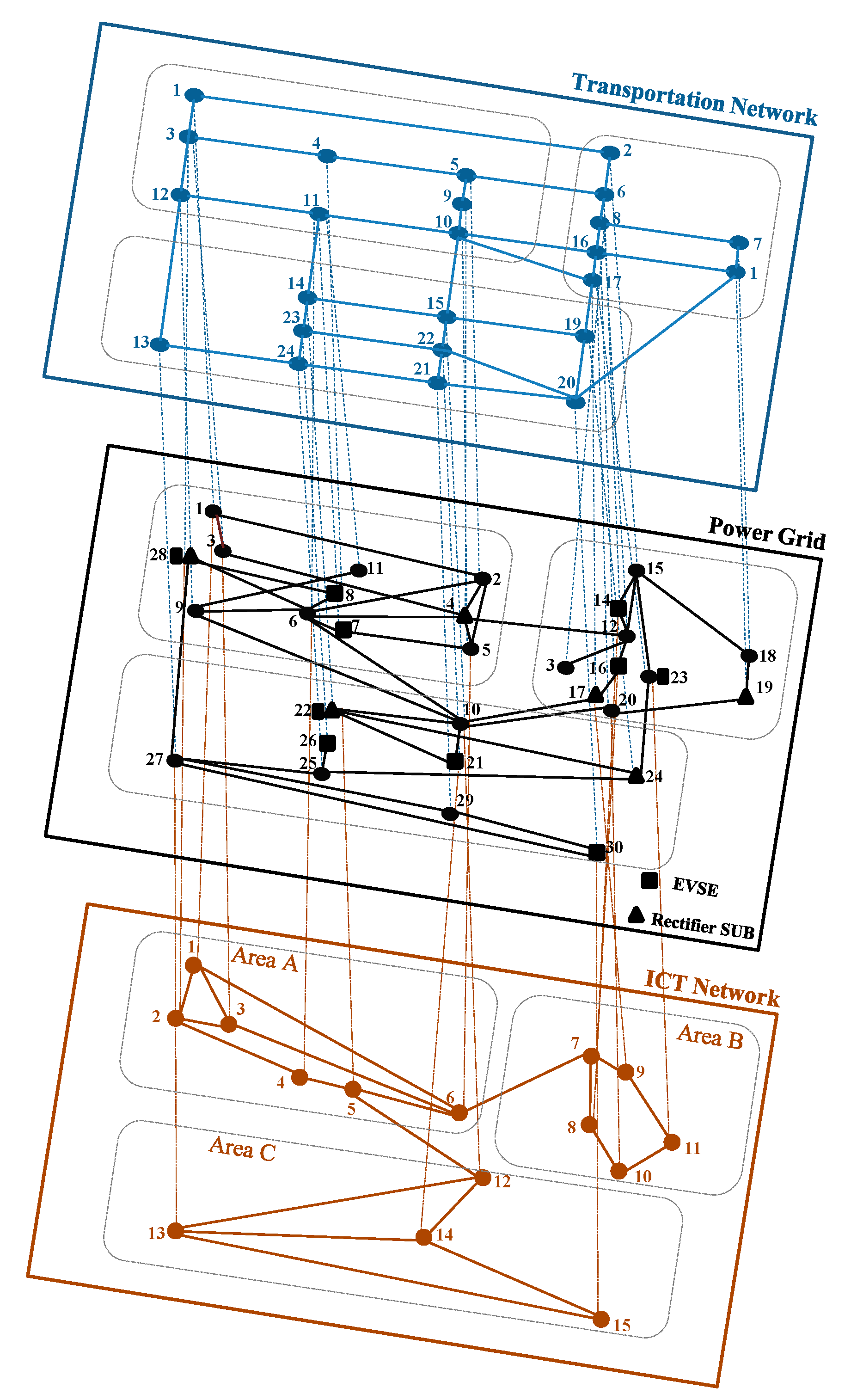
• A new hybrid case study test system that combines a power distribution grid, an ICT network, and a standard transportation test network, which can be used for further analysis and research that integrate these three CIs.

The rest of the paper is organized as follows: in Section 2, the structural and topological interdependencies between the power grid, the ICT network and e-mobility will be modeled; in Section 3, the operational interdependencies will be modeled and the proposed operational influence graph will be presented; in Section 4, a new case study combining the IEEE 30-bus standard distribution network, the 24-node Sioux Falls transportation test network, and an ICT network will be described; in Section 5, results of the case study along with a discussion on the results will be presented; and finally in Section 6, some of the conclusions that can be derived from this study are summarized.

2. Modeling Structural Interdependencies

2.1. Individual Critical Infrastructure (CI) Models

The power grid, the ICT network, and the transportation network will be modeled with three graphs, ${\mathit{G}}_{\mathit{P}}=\left(V_P, E_P\right)$, ${\mathit{G}}_{\mathit{C}}=\left(V_C, E_C\right)$, and ${\mathit{G}}_{\mathit{T}}=\left(V_T, E_T\right)$, respectively. The power grid has $n_P=\left|V_P\right|$ number of power nodes and $l_P=\left|E_P\right|$ number of links; whereas, the ICT network has $n_C=\left|V_C\right|$ number of ICT nodes and $l_C=\left|E_C\right|$ number of ICT links, and the transportation network has $n_T=\left|V_T\right|$ number of transportation nodes and $l_T=\left|E_T\right|$ number of transportation links.

Let $A^P\in {\mathit{R}}^{\left|V_P\right|\times \left|V_P\right|}$, $A^C\in {\mathit{R}}^{\left|V_C\right|\times \left|V_C\right|}$, and $A^T\in {\mathit{R}}^{\left|V_T\right|\times \left|V_T\right|}$ be the adjacency matrices for the power grid, ICT network and transportation network, respectively. The value of $A_{ij}^P$ is 1, as long as a link $e_{ij}^P\in E_P$ exists between nodes $v_i^P\in V_P$ and $v_j^P\in V_P$, and zero otherwise. Since the three CIs are modeled with undirected graphs, the values of $A_{ij}^P=A_{ji}^P$, and $A_{ii}^P=0, \forall \left(i, j\right)\in {\mathit{Z}}_{+}^{\left|E_P\right|}$. Similarly, $A_{ij}^C$ is 1, as long as a link $e_{ij}^C\in E_C$ exists between nodes $v_i^C\in V_C$ and $v_j^C\in V_C$, and zero otherwise. In addition, $A_{ij}^C=A_{ji}^C$ and $A_{ii}^C=0, \forall \left(i, j\right)\in {\mathit{Z}}_{+}^{\left|E_C\right|}$. Finally, $A_{ij}^T$ is 1, as long as a link $e_{ij}^T\in E_T$ exists between nodes $v_i^T\in V_T$ and $v_j^T\in V_T$, and zero otherwise. Also, $A_{ij}^P=A_{ji}^P$, and $A_{ii}^P=0, \forall \left(i, j\right)\in {\mathit{Z}}_{+}^{\left|E_T\right|}$. The Laplacian matrix ${\Gamma }^P$ for $G_P$ can be defined as ${\Gamma }^P=D^P-A^P$, where $D^P$ is a diagonal degree matrix, such that $D_{ii}^P$ equals the degree of node i. Therefore, ${\Gamma }_{ii}^P=D_{ii}^P$, and ${\Gamma }_{ij}^P=-1$ if $v_i^P$ is adjacent to $v_j^P$ (i.e., $A_{ij}^P=1$), and zero otherwise. Similarly, the Laplacian matrices for $G_C$ and $G_T$ can be defined as ${\Gamma }^C=D^C-A^C$ and ${\Gamma }^T=D^T-A^T$, respectively.

Power nodes $V_P$ can be categorized into: 1) generator nodes, $V_G^P\subset V_P$; 2) non-dispatachable load nodes, $V_{NDL}^P\subset V_P$; 3) dispatchable load nodes, $V_{DL}^P\subset V_P$; 4) distributed energy resource nodes, $V_{DER}^P\subset V_P$; 5) microgrid nodes, $V_{\mu G}^P\subset V_P$; 6) electric vehicle supply equipment (EVSE) nodes, $V_{EVSE}^P\subset V_P$; 7) rectifier substations nodes, $V_{Rc}^P\subset V_P$ (supplying the subway system); and 8) downstream main infeed nodes (i.e., connection to a higher-voltage grid), $V_{IN}^P\subset V_P$. A microgrid, by definition, includes one or more DERs, an energy storage system (ESS), and a microgrid central controller (MGCC). A community microgrid is an extended version of the microgrid, where multiple neighboring nodes form an island with clearly defined electrical boundaries, and share resources within a localized transactive energy environment. In normal operation as long as the main grid remains intact, the aggregation is virtual and a community microgrid operates in conjunction with the main grid. When a blackout takes place, a microgrid islands itself and relies on its local resources and controller. A community microgrid hence represents a cut ${\mathit{G}}_{\mathit{P}}^{\mathit{M}}=\left(V_P^M,E_P^M\right)$ of the main graph ${\mathit{G}}_{\mathit{P}}$, where $V_P^M\subset V_P$ and $E_P^M\subset E_P$ are the number of nodes and number of links in the community microgrid, respectively. Dispatchable loads represent loads that can be scheduled to receive power at a later time, unlike the conventional non-dispatchable loads that receive their power on demand.

The ICT nodes $V_C$ can be categorized into measurement nodes $V_{\mathbb{Z}}^C\subset V_C$, router nodes $V_{ℝ}^C\subset V_C$, and control center nodes $V_{ℂ}^C\subset V_C$. $V_{\mathbb{Z}}^C$ nodes are where measurement devices, typically line flow, bus injection and bus voltage magnitude, are placed. The $V_{ℝ}^C$ nodes route the messages coming from various $V_{\mathbb{Z}}^C$ on their way to one of the control centers $V_{ℂ}^C$, where data processing and decision-making take place.

The e-mobility nodes can be categorized into road junctions $V_{\mathfrak{j}}^T\subset V_T$ and train passenger stations $V_{\mathfrak{s}}^T\subset V_T$. The set of links $E_T$ include road sections between adjacent junctions $E_{\mathfrak{j}}^T\subset E_T$ and train railway sections between adjacent stations $E_{\mathfrak{s}}^T\subset E_T$. Some $V_{\mathfrak{j}}^T$ nodes may include EVSE nodes $V_{EVSE}^T\subset V_{\mathfrak{j}}^T$.

2.2. The Integrated Structural Interdependency Model

The integrated graph ${𝓖}_S=\left({\mathbb{V}}_S,{\mathbb{E}}_S\right)$ relates the three CIs through a set of structural interdependency links ${ℐ}_S$. Note that ${𝓖}_S\supset \left\{{\mathit{G}}_{\mathit{P}},{\mathit{G}}_{\mathit{C}},{\mathit{G}}_{\mathit{T}}\right\}$ such that ${\mathbb{V}}_S=\{V_P{\cup }^{}{V}_C{\cup }^{}{V}_T\}$ and ${\mathbb{E}}_S=\{E_P{\cup }^{}{E}_C{\cup }^{}{E}_T{\cup }^{}{ℐ}_S\}$. The set of interdependency links between the power grid and the ICT network ${ℐ}_S^{PC}\subset {ℐ}_S$ link power nodes to their corresponding ICT nodes (i.e., the nodes that deliver measurements and control decisions back and forth between the power nodes and the control center). They also indicate the dependence of ICT nodes on the power grid for power supply. The interdependency links between the power grid and the transportation network ${ℐ}_S^{PT}\subset {ℐ}_S$ link the power nodes to transportation ones (e.g., they indicate which passenger stations or EVSEs are being supplied by which power substations). A link exists between an EVSE power node $V_{EVSE}^P$ and the junction where the EVSE is geographically located $V_{\mathfrak{j}}^T$ on the transportation network. Links to further adjacent transportation junctions to the EVSE junction $V_{\mathfrak{j}}^T$ are also considered, since the focus of this paper is on urban region with short distances between adjacent nodes. In the subway system, rectifier substations are typically geographically distributed throughout the various subway lines to maintain regulation of the supply voltage. The number of rectifier substations is smaller than the number of passenger stations. It is assumed here that a rectifier substation power node $V_{Rc}^P$ is affected by two neighboring passenger stations on each side, except for the terminal substations, which are affected by two passenger stations on one side only. The impact of the adjacent passenger stations is higher (~double) of the farther ones. The integrated graph ${𝓖}_S$ may be directly used to infer some of the characteristics of the interdependency between the three CIs, e.g., using centrality measures. However, ${𝓖}_S$ will be built upon and an influence graph will be developed, which considers operational aspects in addition to the topological ones encompassed within ${𝓖}_S$.

3. Modeling Operational Interdependencies

The structural interdependency models, described in Section 2, provide a good insight on the geographical and topological relations among nodes. Nonetheless, they may not be enough to describe the propagation of failures in the power grid, since cascaded failures do not resemble contagion or epidemic behavior. Failure of a component in the power grid may lead to a failure of another component that is substantially far, both geographically and/or topologically.

Moreover, the load demand of the power grid considerably contributes to determining the interdependencies between nodes and links. For instance, if a link of the power grid fails, the power that the failed line was carrying before braking would be shifted to other transmission line/s increasing the amount of power flowing through them. Whether this increase in power flow will lead another link to fail or not, depends on how much power it was delivering to the loads, at the moment of disturbance. Therefore, it is rather unpersuasive to assume that the topology of the power grid is solely enough to realistically capture the behavior of the power grid during failure propagation.

3.1. Interdependency Influence Graphs

In this paper, the operational interdependencies will be modeled with weighted temporal influence graphs. The power grid will be modeled with ${\mathit{G}}_{\mathit{P}}^{\mathit{I}}\left(t,G_P^t\right)=\left(V_P, V_P^l, V_P^{Ⅎ}, E_P^I\right)$. $G_P^I$ changes over time due to load/generation changes. In addition, it changes as the topology of $G_P$ changes (e.g., due to line or node disconnection). $G_P^I$ can be modeled as a continuous series of static networks (i.e., snapshots). In this hybrid state/event driven model, a new snapshot is formed if: 1) some predefined time interval $\left(T_S\right)$ passes, e.g., $T_S$ may be a few minutes, transitioning $G_P^I$ from $G_P^I\left(t,G_P^t\right)$ to $G_P^I\left(t+T_S,G_P^t\right)$; and/or 2) a contingency takes place in the power grid, transitioning $G_P^I$ from $G_P^I\left(t,G_P^t\right)$ to $G_P^I\left(t,G_P^{t+1}\right)$. $G_P^I$ has $n_P^I=\left|V_P+V_P^l+V_P^{Ⅎ}\right|$ number of nodes and $l_P^I=\left|E_P^I\right|$ number of links. The $V_P^l\in {\mathit{R}}^{1\times \left|V_P\right|}$ nodes in $G_P^I$ represent the links of $G_P$, i.e. in the proposed influence graph, both the power grid’s buses (nodes) and lines (links) are modeled as nodes. The $V_P^{Ⅎ}$ set includes fictitious nodes that will be added to $G_P^I$ to model alternative sources of power, as in the case of microgrid nodes. $E_P^l{}_{ij}$ varies between 0 and 1, and signifies the tendency of node $V_P^l{}_i$ to fail following a disturbance at node $V_P^l{}_j$. The fundamental question here is how to establish the weights of $E_P^I$. The links $E_P^l\in {\mathit{R}}^{\left|V_P+V_P^l\right|\times \left|E_P^I\right|}$ represent a time-varying failure propagation index (FPI) between nodes, throughout the network.

3.2. Failure Propagation Index (FPI)

The FPI index between the various nodes of $G_P^I$ will be calculated as follows:

(1) To calculate the set of edges $E_{LP}^P\subset E_P^I$ from the $V_P^l$ nodes to the $V_P$ ones, the degree of the $V_P$ node and the line loading of its adjacent links are taken into consideration. $E_{LP}^P$ edges represent the FPI of a node, following the failure of a link. Note that every $V_P^l$ node can be mapped to an $E_P$ link of $G_P$.

$$E_{LP}^P\left(j,i\right)=\{\begin{array}{cc}1& \mathrm{if} D_{ii}^P=1 \vee E_{LP}^P>1\\ \left|P_i\right|/{\displaystyle {\displaystyle \sum }_{D_{ii}^P-1 | k\ne i}}\left|F_{ik}-C_{ik}\right|& \mathrm{if} D_{ii}^P>1 | A_{ik}^P=1\end{array}$$

(1a)

$$P_i={\displaystyle \sum }_{D_{ii}^P}{F}_{ik} \forall k : A_{ik}^P=1$$

(1b)

$$P_i=\mathit{B}\mathsf{\delta }$$

(1c)

$$\tilde{\mathsf{\delta }}={\tilde{\mathit{B}}}^{-1}\widetilde{P_i}$$

(1d)

$$F=H\tilde{\mathsf{\delta }}$$

(1e)

where $P_i$ is the net power injection at node $i$, $F_{ik}$ is the power flow through the link connecting nodes $i$ and $k$, and $C_{ik}$ is the power flow capacity of the same link. (1b) denotes the nodal power balance, (1c) relates $P_i$ to the imaginary component of the bus admittance matrix ($\mathit{B}$) and the phase angle $\mathsf{\Delta }$ at every bus. In (1d), $\tilde{\mathsf{\delta }}$, ${\tilde{\mathit{B}}}^{-1}$, and $\widetilde{P_i}$ extend (1c) when the elements (row and column) attributed to the reference bus (i.e., a bus with a slack generator) are eliminated from $\mathsf{\delta }$, $\mathit{B}$, and $P_i$, respectively. Finally, $F$ can be calculated using 1e.

This expression tends to one, when the failing link supports the only connection between the node and the rest of network. In other words, if a node is connected to the network through a single link as in the case of a node located at the end of a radial distribution feeder, failure of the link will inevitably lead to failure of the node. If a node is connected to more than a single link, failure of a link may or may not impact the node, depending on the remaining capacity margin of its adjacent lines combined. Note the absolute sign of the term $\left|P_i\right|$ denoting that the expression can be generalized to both load and generator nodes.

(2) To calculate the set of edges $E_{PL}^P\subset E_P^I$ from the $V_P$ nodes to the $V_P^l$ ones, the FPI here will represent the sensitivity of line loading to node power variations. Note from (1d) and (1e) that:

$$\Delta F=H{\tilde{\mathit{B}}}^{-1} \Delta \widetilde{P_i}$$

(2a)

$$\mathbb{S}=H{\tilde{\mathit{B}}}^{-1}$$

(2b)

$\Delta F$ is a vector combining the power variation in the various lines for changes in the power injection vector $\Delta \widetilde{P_i}$. $\mathbb{S}$ may be directly used to estimate $E_{PL}^P$; however, we can also adhere to the deterministic flow-based approach of this paper and attempt to include the actual power flow, as follows.

$$E_{PL}^P\left(j,i\right)=\{\begin{array}{cc}1& \mathrm{if} E_{PL}^P>1\\ \left|{\mathbb{S}}_{ij} \Delta \widetilde{P_i}\right|/\left|F_{ij}-C_{ij}\right|& \mathrm{otherwise}\end{array}$$

(3)

(3) To calculate the set of edges $E_{LL}^P\subset E_P^I$ from the $V_P^l$ nodes to other $V_P^l$ ones, the FPI here will represent the sensitivity of line loading of each line to failure of other lines. This can be computed by modifying $\mathbb{S}$, multiplying it by the node-branch incidence matrix, to represent $\mathbb{S}$ of line $F_{ik}$ to power injection at bus $k$. A line outage distribution factor $\mathit{\varsigma }$ can then be represented as follows.

$$\Delta {\overbrace{F}}_{L_i}={\mathit{\varsigma }}_{L_i{L}_j} \Delta {\overbrace{F}}_{L_j}^{\left({\tau }_{c-}\right)}$$

(4)

$\overbrace{F}$ is an array combining all elements of $F$ as a vector. ${\mathit{\varsigma }}_{L_i{L}_j}$ relates the change in the loading of line $L_i$ following the loss of line $L_j$, as a function of the line flow of line $L_j$ just before the contingency incident ${\tau }_c$.

$$E_{LL}^P\left(L_i,L_j\right)=\{\begin{array}{cc}1& \mathrm{if} E_{LL}^I>1\\ \left|{\mathit{\varsigma }}_{L_i{L}_j} \Delta {\overbrace{F}}_{L_j}^{\left({\tau }_{c-}\right)}\right|/\left|F_{L_j}-C_{L_j}\right|& \mathrm{otherwise}\end{array}$$

(5)

The values of $E_P^I$ are limited to one in this paper, for visualization and comparison purposes. This limit is nevertheless optional and may be eschewed if needed.

3.3. Microgrids and Energy Storage Systems

Unlike $V_G^P$, $V_{NDL}^P$, $V_{DL}^P$, $V_{DER}^P$, and $V_{IN}^P$, the set of $V_P$ nodes with an energy storage system (ESS) or microgrid $V_{\mu G}^P\subset V_P$ require special attention since the energy storage capability raise their resiliency level and reduce the FPI. Note that the $V_{EVSE}^P$ may need to be treated similar to $V_{\mu G}^P$ if an ESS is deployed (i.e., as in the case of direct current (DC) fast charging stations) or when EVs within an EVSE participate in V2X services, such as V2G, V2V or V2B. For every $V_{\mu G}^P$ node, a $V_P^{Ⅎ}$ node is introduced that will connect to the microgrid node via a single link. The $V_P^{Ⅎ}$ connects to $G_P^I$ only through the microgrid node. Following the failure of its adjacent lines, the probability that a microgrid node fails heavily depends on the availability of energy from its local energy sources, including ESS and DERs. The set of links $E_{P\mu }^P\subset E_P^I$ between a microgrid node $i\in V_{\mu G}^P$ and its corresponding fictitious node $\breve{i}\in V_P^{Ⅎ}$ can be calculated as follows.

$$E_{P\mu }^P(i,\breve{i})=\{\begin{array}{cc}0\hfill & \mathrm{if} P_{\mu G}^{\left({\tau }_{c-}\right)}=0 \vee \left|P_i\right|\le {\displaystyle {\displaystyle \sum }_{D_{ii}^P}}\left|F_{ik}-C_{ik}\right|\hfill \\ {\mathcal{A}}_i\left|P_{\mu G}^{ℳ}\right|/\left(\left|P_i\right|-{\displaystyle {\displaystyle \sum }_{D_{ii}^P}}\left|F_{ik}-C_{ik}\right|\right)\hfill & \mathrm{if} \left|P_i\right|>{\displaystyle {\displaystyle \sum }_{D_{ii}^P}}\left|F_{ik}-C_{ik}\right|\hfill \\ 1\hfill & \mathrm{if} E_{P\mu }^P>1\hfill \end{array}$$

(6)

$P_{\mu G}^{ℳ}$ is the maximum power capacity of the local resources, i.e., ESS and/or DERs, combined. $\mathcal{A}\in \left[0,1\right]$ is a time-varying availability factor that takes into account energy availability parameters, including current and forecasted renewable energy production, ESS state of charge, ESS charging/discharging rates, etc.

3.4. The Integrated Operational Interdependency Model

The integrated influence graph ${𝓖}_{ℐ}=\left({\mathbb{V}}_{ℐ},{\mathbb{E}}_{ℐ}\right)$ models the operational interdependencies between the three CIs through links ${ℐ}_{ℐ}$. The set of directed interdependency links between the power grid and the ICT network ${ℐ}_{ℐ}^{PC}\subset {ℐ}_{ℐ}$ models the influence of power nodes on ICT ones and vice versa; whereas, ${ℐ}_{ℐ}^{PT}\subset {ℐ}_{ℐ}$ models the operational interdependency between the power grid and the transportation network. The ICT network will be modeled via ${\mathit{G}}_{\mathit{C}}^{\mathit{I}}=\left(V_C, E_C^I\right)$. $E_C^I$ are links that determine the influence of ICT nodes on each other, analogues to $E_P^I$ in $G_P^I$. We will calculate $E_C^I$ between nodes $i\in V_C$ and $j\in V_C$ using (7), considering the degree of node $i$, $D_{ii}^C$. $j\in V_C$ is a node that lies on one of the paths connecting node $i$ to the control center. Even though this may be considered a topological factor, it will be adopted in this paper for simplicity. However, other operational factors of the ICT network, e.g., delay or packet loss, may be also be considered.

$$E_C^I\left(i,j\right)=1/{\Re }_i^C$$

(7)

${\Re }_i^C$ is the set of possible shortest paths between node $i$ and the control center, excluding those that will not be available due to failure of node $j$. The power grid measurements, which are needed by the power grid operator to make proper control decisions, are transmitted from measurement devices to the control center through ICT nodes. The interdependency links originating from the ICT nodes to the power grid ones will be calculated to signify the impact of a lost ICT node on the observability of the power grid. We define $𝓈=\left(\delta ;\phi ;\mathcal{V};ℛ\right)\in \mathit{R}$ as the state vector of the power grid at a given time, $\phi$ is a vector of transformer phase shifts, $\mathcal{V}$ is the voltage magnitude at every bus, and $ℛ$ is a vector of transformer off-nominal voltage ratios. The set of measurements $𝓂$ can be modeled as $𝓂=𝒽(𝓈)+\epsilon$. The measurement errors $\epsilon$ are typically minimized using weighted least square formulation as follows.

$$\mathsf{\zeta }=\frac{1}{2}{\left[𝓂-𝒽(𝓈)\right]}^T{\mathsf{\Lambda }}^{-1}\left[𝓂-𝒽(𝓈)\right]$$

(8)

This can be approached by recursively solving (8), using the Newton’s method.

$${𝓈}^{v+1}={𝓈}^v+{𝓑}_v^{-1}{\mathscr{H}}_v\left[𝓂-𝒽\left({𝓈}^v\right)\right]$$

(9a)

$${\mathscr{H}}_v=\nabla 𝒽\left({𝓈}^v\right)$$

(9b)

$${𝓑}_v={\mathscr{H}}_v^T{\Lambda }^{-1}{\mathscr{H}}_v$$

(9c)

$\Lambda$ is a square matrix whose off-diagonal elements are zeros, and diagonal elements equal the standard deviation of the measurement errors, and $v$ is the iteration index. The observability of the power grid depends on the rank of ${𝓑}_v$. Therefore, the link from a power grid node $i$ to an ICT node $j$, ${ℐ}_{ℐ}^{C⟶P}\left(i,j\right)\subset {ℐ}_{ℐ}^{PC}$ is attained by calculating ${𝓻}^{\left({\tau }_{c-}\right)}=\mathrm{rank}({𝓑}_v^{\left({\tau }_{c-}\right)})$ before ICT node failure, and ${𝓻}^{\left({\tau }_{c+}\right)}=\mathrm{rank}({𝓑}_v^{\left({\tau }_{c+}\right)})$ after node failure.

$${ℐ}_{ℐ}^{C⟶P}=\{\begin{array}{cc}{ℯ}_i^C& \mathrm{if} {𝓻}^{\left({\tau }_{c+}\right)}<{𝓻}^{\left({\tau }_{c-}\right)}\\ \frac{1}{{\mathfrak{l}}_i^C}& \mathrm{otherwise}\end{array}$$

(10)

${\mathfrak{l}}_i^C$ is the number of ICT nodes connected to power node $i$. ${ℯ}_i^C\in \left[0,1\right]$ is the estimated error between the actual measurement of $i$, and its estimated value. This can be approached by analyzing the variability/predictability of historical profiles for the power injection at the node. Several factors may be taken into consideration, such as whether it is a load bus, or a DER one with intermittent solar generation. The interdependency link from an ICT node $i$ to a power grid node $j$, ${ℐ}_{ℐ}^{P⟶C}\left(i,j\right)\subset {ℐ}_{ℐ}^{PC}$ is obtained by considering the dependency of the ICT node on the power from the power one, and whether there is a local back up resource at the communication node or not.

$${ℐ}_{ℐ}^{P⟶C}=\frac{1}{{\mathfrak{l}}_i^P}$$

(11)

where ${\mathfrak{l}}_i^P$ is the number of power nodes connected to ICT node $i$. If the state of the power grid is unobservable following an ICT failure, the system may actually be divided into multiple observable islands. In order for the power grid operator to be able to yield a control decision before the current control cycle times out, some pseudo-measurements (e.g., an estimated nodal power injection, replacing a missing measured value) must be introduced. Control decisions that are based on many pseudo-measurements may not be accurate, especially during large power grid disturbances. A more accurate way to find ${ℐ}_{ℐ}^{C⟶P}$ might be achieved by simulating the power grid under various ICT node failures, and estimating the impact of inaccurate control resulting from node failures on line congestions.

If a backup source is available at an ICT node, a fictitious power node $\breve{i}$ is added, to supply its designated ICT node only. The link between the ICT node $i$ and the added node $\breve{i}$ can be obtained as follows.

$$E_C^{Ⅎ}(i,\breve{i})=\frac{{\mathcal{D}}_i{T}_s}{\mathcal{C}\left(\mathsf{\Psi }-{\mathsf{\Psi }}^{min}\right)}$$

(12)

where $\mathcal{C}$ is the total energy capacity, and $\mathsf{\Psi }$ is the current available energy level (e.g., state of charge (SoC) in the case of a battery). An ICT node is not solely dependent on the power grid to remain functional if it has local back up generation; however, during a blackout the health of the node will depend on the availability of energy from the local resources.

The transportation network will be modeled via ${\mathit{G}}_{\mathit{T}}^{\mathit{I}}=\left(V_T,V_T^l, E_T^I\right)$. The $V_T^l$ nodes represent the links $E_T$ of $G_T$. $E_{TL}^T\subset E_T^I$ represents a set of links between a $V_T$ node and a $V_T^l$ one. $E_{LL}^T\subset E_T^I$ represents a set of links between a $V_T^l$ node and another $V_T^l$ one. No direct links are considered between $V_T$ nodes. The $V_T^l$ nodes can be categorized into nodes $V_T^{\mathfrak{j}}\subset V_T^l,$ which map the $E_{\mathfrak{j}}^T$ links, and nodes $V_T^{\mathfrak{s}}\subset V_T^l$ that map the $E_{\mathfrak{s}}^T$ ones.

The link $E_{TL}^T$ between a node $i\in V_T$ and another $j\in V_T^l$ is set to 1—that is, the failure/congestion of a junction or passenger station will lead to the failure of its adjacent road/rail sections; hence, forcing drivers to go through other nodes. On the other hand, the link $E_T^I$ originating from a node $j\in V_T^l$ to a node $i\in V_T$ shall be calculated as follows:

$$E_{TL}^T\left(j,i\right)=1/D_{ii}^T$$

(13)

The mobility of travelers plays a major role in defining the characteristics of the transportation system, and its interdependencies with the other CIs. In an urban region, there may be three main modes of morning and evening commutes: on foot, by automobile (including regular and electric public transit buses, personal cars and EVs, and regular and electric taxicabs), and by electric railway system (i.e., subway). Those who move on foot may not have a significant impact on CIs. However, the automobile and subway modes are interrelated; consider a group of passengers traveling from a certain origin to a destination, if they drive or take a taxicab or bus, the loading on the subway system is reduced, and vice versa. Failure of a subway passenger station that is serving an area may lead to traffic congestion around it since people would commute by automobile. In a system with a high level of penetration of EVs, this scenario consequently leads to increased charging demand from EVs and electric buses, which reflects on the power grid. By contrast, during power grid full or partial outage, some EVSEs may not be available. The demand on the subway system may substantially increase, potentially leading to one of two problems: 1) the subway system operator may increase the frequency of the trains to accommodate the high demand, increasing the power demand of associated substations; and 2) the subway system may not increase the frequency of the trains, leading to extensive travel delays (and economic loss as a consequence). Therefore, it is essential to model the links between the $V_T^{\mathfrak{j}}$ nodes and the $V_T^{\mathfrak{s}}$ ones. The $E_{LL}^{\mathfrak{j}\mathfrak{s}}\left(i,j\right)\in E_{LL}^{\mathfrak{j}\mathfrak{s}}\subset E_{LL}^T$ link from node $i\in V_T^{\mathfrak{j}}$ to node $j\in V_T^{\mathfrak{s}}$ is calculated by (14); whereas, the $E_{LL}^T\left(j,i\right)\in E_{LL}^{\mathfrak{s}\mathfrak{j}}\subset E_{LL}^T$ link from $j\in V_T^{\mathfrak{s}}$ to $i\in V_T^{\mathfrak{j}}$ is given by (15).

$$E_{LL}^{\mathfrak{j}\mathfrak{s}}\left(i,j\right)=\{\begin{array}{cc}1& \mathrm{if} E_{LL}^{\mathfrak{j}\mathfrak{s}}>1\\ \left|{\sigma }_{ij}^{\mathfrak{j}\mathfrak{s}}\Delta {\mathfrak{E}}_{ij}^{\mathfrak{j}}\right|/\left|{\mathfrak{E}}_{ij}^{\mathfrak{s}}-C_{ij}^{\mathfrak{s}}\right|& \mathrm{otherwise}\end{array}$$

(14)

$$E_{LL}^{\mathfrak{s}\mathfrak{j}}\left(i,j\right)=\{\begin{array}{cc}1& \mathrm{if} E_{LL}^{\mathfrak{s}\mathfrak{j}}>1\\ \left|{\sigma }_{ij}^{\mathfrak{s}\mathfrak{j}}\Delta {\mathfrak{E}}_{ij}^{\mathfrak{s}}\right|/\left|{\mathfrak{E}}_{ij}^{\mathfrak{j}}-C_{ij}^{\mathfrak{j}}\right|& \mathrm{otherwise}\end{array}$$

(15)

$\Delta {\mathfrak{E}}_{ij}^{\mathfrak{j}}$ represents the change in the flow due to a problem in the $E_{\mathfrak{j}}^T\left(i,j\right)$ link, which may overload link $E_{\mathfrak{s}}^T\left(i,j\right)$ with a probability of ${\sigma }_{ij}^{\mathfrak{j}\mathfrak{s}}$. The term $\left|{\mathfrak{E}}_{ij}^{\mathfrak{j}}-C_{ij}^{\mathfrak{j}}\right|$ represents the remaining capacity of link $E_{\mathfrak{s}}^T\left(i,j\right)$. In other words, when road link $E_{\mathfrak{j}}^T\left(i,j\right)$ fails, travelers may commute with a probability ${\sigma }_{ij}^{\mathfrak{j}\mathfrak{s}}$ using the subway link $E_{\mathfrak{s}}^T\left(i,j\right)$. This will increase the demand on the subway system, and require an increase in the frequency of the trains. Whether this change in the mode would overburden the subway link or not, depends on the initial loading condition of that link. $\Delta {\mathfrak{E}}_{ij}^{\mathfrak{s}}$ represents the change in the traffic low in the $E_{\mathfrak{s}}^T\left(i,j\right)$ link, which may overload link $E_{\mathfrak{j}}^T\left(i,j\right)$ with a probability of ${\sigma }_{ij}^{\mathfrak{s}\mathfrak{j}}$. Similarly, the term $\left|{\mathfrak{E}}_{ij}^{\mathfrak{s}}-C_{ij}^{\mathfrak{s}}\right|$ represents the remaining capacity of link $E_{\mathfrak{j}}^T\left(i,j\right)$.

EVs charge at EVSEs whose power supply is part of the power grid, $V_{\mathit{EVSE}}^P\subset V_P$. The number of cars charging at an EVSE, and consequently the power demand at its corresponding $V_{EVSE}^P$ node, is affected by the transportation network. For instance, if the path leading to an EVSE is blocked or congested, the EVs seeking charge at that EVSE will likely travel to the nearest functional EVSE. This functional EVSE will experience more than normal demand, potentially overloading the power substations supplying them. On the other hand, if some EVSEs are not functional within an area (e.g., due to malfunction of the power substations supplying them), traffic may be congested around the functional EVSEs. This effect may be more severe during natural disasters, similar to a familiar scenario when cars get packed at gas stations with functional back up pumping power, during natural disasters and blackouts. To model the dependence of the power grid on the transportation network, we will introduce links between the $E_T^I$ links, and the $E_P^I$ ones. When a transportation link $E_T^I$ leading to an EVSE or a passenger station fails, the load may be redirected to the nearest transportation node (junction or passenger station), and consequently impact another power node. The impact on the power grid will then depend on the available capacities of the power links adjacent to that power node. When a link $i\in E_T^I$ fails, and that link is leading to an EVSE or a passenger station, such that its nearest alternate node is $j\in E_T^I$, the link between the transportation node and the power links around $j$, ${ℐ}_{ℐ}^{T⟶P}\left(i,j\right)$, can be calculated as follows:

$${ℐ}_{ℐ}^{T⟶P}=\{\begin{array}{cc}1& \mathrm{if} {ℐ}_{ℐ}^{T⟶P}>1\\ \left|{\sigma }_{ij}^{\mathfrak{j}\mathfrak{j}}\Delta {\mathfrak{E}}_{ij}^{\mathfrak{j}}{\mathcal{D}}_{ij}^{\mathfrak{j}}+{\sigma }_{ij}^{\mathfrak{s}\mathfrak{s}}\Delta {\mathfrak{E}}_{ij}^{\mathfrak{s}}{\mathcal{D}}_{ij}^{\mathfrak{s}}\right|/{\displaystyle {\displaystyle \sum }_{D_{jj}^P :\exists A_{jk}^P=1}}\left|F_{ik}-C_{ik}\right|& \mathrm{otherwise}\end{array}$$

(16)

${\sigma }_{ij}^{\mathfrak{j}\mathfrak{j}}\Delta {\mathfrak{E}}_{ij}^{\mathfrak{j}}$ and ${\sigma }_{ij}^{\mathfrak{s}\mathfrak{s}}\Delta {\mathfrak{E}}_{ij}^{\mathfrak{s}}$ represent the new (transportation) demand encountered by node junctions and passenger stations located nearest to node $j$, respectively, following the failure of link $i$. ${\mathcal{D}}_{ij}^{\mathfrak{j}}$ and ${\mathcal{D}}_{ij}^{\mathfrak{s}}$ represent the power demand per unit increase in the traffic and subway demand. ${\mathcal{D}}_{ij}^{\mathfrak{j}}$ may be considered as a stochastic variable that correlates the traffic flow at a road, to the charging demand at an existing EVSE. ${\mathcal{D}}_{ij}^{\mathfrak{s}}$ may be calculated in a more deterministic manner, since we can relatively easily relate the trains’ frequency to the demand of the rectifier substations looking at real-time measurements or historical interval data.

To model the dependence of the transportation network on the power grid, we will introduce links between both of the $V_{EVSE}^P$ and $V_{Rc}^P$ nodes, and the $E_T^I$ links, ${ℐ}_{ℐ}^{P⟶T}$. When an EVSE node $i\in V_{EVSE}^P$ fails, the $E_T^I$ link leading to the nearest EVSE node $j\in V_{EVSE}^P$ will be impacted. This dependence will be modeled by a link ${ℐ}_{ℐ\mathfrak{j}}^{P⟶T}\left(i,j\right)\subset {ℐ}_{ℐ}^{P⟶T}$.

$${ℐ}_{ℐ\mathfrak{j}}^{P⟶T}\left(i,j\right)=\{\begin{array}{cc}1& \mathrm{if} {ℐ}_{ℐ\mathfrak{j}}^{T⟶P}\left(i,j\right)>1\\ \left|{\sigma }_{ij}^{\mathfrak{j}\mathfrak{j}}\Delta {\mathfrak{E}}_{ij}^{\mathfrak{j}}\right|/\left|{\mathfrak{E}}_{ij}^{\mathfrak{j}}-C_{ij}^{\mathfrak{j}}\right|& \mathrm{otherwise}\end{array}$$

(17)

When a rectifier substation node $i\in V_{Rc}^P$ fails, its neighboring substations have to accommodate the load that the failed substation was handling before failure. Depending on the strength of the power supply of the subway system (number and distribution of substations, short circuit impedance of the substations, etc.), the voltage of the subway system supply rail (e.g., the third rail in a DC electric rail system) may drop. In this case, the impacted section of the subway system may shut down. Whether the neighboring substations can maintain the voltage or not, relies on how much power they were carrying before the fault and their maximum capacity, and how far those substations are from the failing one. Note that a neighboring substation may not be capable of supporting a failing one, even though it has enough power capacity, if the failed substation is far. Distance creates losses and voltage drop that may trigger the under-voltage protection devices, especially if uncontrolled rectifiers are used, which is the case in many electric rail transit systems. When rectifier substation node $i\in V_{Rc}^P$ fails, the $E_T^I$ links adjacent to it may fail if the nearest rectifier substation node $j\in V_{Rc}^P$ cannot remotely regulate the voltage at $i$. This dependence will be modeled by a link ${ℐ}_{ℐ\mathfrak{s}}^{P⟶T}\left(i,j\right)\subset {ℐ}_{ℐ}^{P⟶T}$. This process is heavily impacted by the frequency of the trains, i.e., during morning or evening peaks when frequency of the trains is high, the voltage generally tends to drop, and failure of a substation may be severe.

$${ℐ}_{ℐ\mathfrak{s}}^{P⟶T}\left(i,j\right)=\{\begin{array}{cc}1& \mathrm{if} {ℐ}_{ℐ\mathfrak{j}}^{P⟶T}\left(i,j\right)>1\\ \left|{\sigma }_{ij}^{\mathfrak{s}\mathfrak{s}}\Delta {\mathfrak{E}}_{ij}^{\mathfrak{s}}{\mathcal{D}}_{ij}^{\mathfrak{s}}\right|/{\varkappa }_{ji}\left|P_j^{ℳ}-P_j\right|& \mathrm{otherwise}\end{array}$$

(18)

${\varkappa }_{ji}$ represents the probability that rectifier substation $j\in V_{Rc}^P$ can support a failed substation $i\in V_{Rc}^P$, which can be estimated by simulating the system under various loading (trains/hour) and contingency scenarios [24].

4. Case Study

The proposed modeling approach will be tested on a benchmark problem that the author has presented in [25], by overlaying the Sioux Falls 24-node transportation test network onto the standard IEEE 30-bus test feeder, and an ICT network as shown in Figure 1. This multilayered test system will be referred to as the “Aggregated Model.” This study region is divided into three main urban agglomerations, namely: Area A, Area B, and Area C. These areas are further broken down into various geographically distributed zones. Each area is supplied via some local generators through distribution lines. Moreover, there is a tie line that enables energy exchange between Areas A and B, three tie lines between Areas B and C, and three tie lines between Areas C and A. Bus 1 represents the interface between the power distribution grid, and the higher-voltage bulk power transmission system. Bus 1 also serves as the slack in normal operating conditions. The DMS is assumed to be located near bus 1. There are 30 buses (i.e., power grid nodes), and 41 distribution lines/cables (i.e., power grid links). Buses {1, 2, 3, 4, 5, 6, 7, 8, 9, 11, 28} lie within Area A, buses {12, 13, 14, 15, 16, 7, 18, 19, 20, 23} lie within Area B, and buses {10, 21, 22, 24, 25, 26, 27, 29, 30} lie within Area C.

There are 3 solar photovoltaic systems located at buses 2 (Area A), 13 (Area B), and 22 (Area C). There are 7 EVSEs located at buses 7, 8, 14, 16, 21, 26, and 30. The EVSEs at buses 7, 14, 16, 21, and 30 are assumed to be smart, such that they can reduce their consumption when commanded by the control center, or when energy prices are high [26]. There are 5 rectifier substations supplying the electric rail transit systems, located at buses 7, 12, 19, 22, and 24. There are three microgrids located at buses 28, 23, and 22. The microgrids located at buses 28 and 23 are collaborative; they continuously coordinate with the DMS, sending state measurements and receiving control commands. Moreover, the load at bus 12 is assumed to be dispatchable.

An ICT network is used to collect and transmit real-time measurements from the distribution grid to the DMS, and deliver control decisions from the DMS back to the generators, microgrids, EVSEs, and dispatchable loads. There are 15 ICT nodes, and 20 ICT links. The power injection is measured at buses (i.e., power grid nodes) 1, 3, 5, 6, 14, 16, 17, 20, 10, 15, 21, 27, and 30. The power flow is measured in the distribution lines connecting between nodes (28, 27), (6, 10), (10, 9), (17, 10), and (23, 24).

The 24 nodes of the Sioux Falls test network (i.e., transportation system nodes) represent major junctions, which are interlinked through 38 roads/streets (i.e., transportation system links). Transportation nodes {1, 3, 4, 5, 9, 10, 11, 12} lie within Area A of the power grid; whereas, nodes {2, 6, 7, 8, 16, 17, 18} lie within Area B, and nodes {13, 14, 15, 19, 20, 21, 22, 23, 24} lie within Area C. The EVSEs are located at transportation nodes 4, 12, 6, 16, 20, 22, and 30. In addition, there is a 3-line subway system that links the three areas. Subway Line A$\leftrightarrow$B connects between Areas A and B, and has passenger stations near transportation nodes 12, 11, 9, 8, and 7. Subway Line B$\leftrightarrow$C has stops at transportation nodes 2, 6, 8, 16, 17, 22, 24, and 13. Subway Line C$\leftrightarrow$A has stops at transportation nodes 21, 22, 11, and 1. There are four main public transit bus routes, {1, 3, 12, 13, 24}, {1, 2, 6, 8, 16, 17, 19, 20, 22, 15}, {9, 8, 7, 18, 16, 17, 10}, and {1, 3, 4, 5, 9, 10, 15, 14, 23, 24, 21, 22}.

5. Results and Discussion

The proposed interdependency model was applied on the Aggregated Model. Figure 2 shows the operational interdependency influence graph. While this graph can be presented as a full graph, such that all links within each of the CIs or between CIs are shown, some of the important links are shown in this paper. A good approach here may be to show the links with FPI values of more than a pre-determined threshold (e.g., 0.5), since those with lesser values represent less influence on the rest of the system. The weights of the influence graph represent the impact of a node or link failure on other nodes and links (i.e., the FPI). Therefore, navigating through this graph starting from a node provides an insight on how a failure initiated at that node may propagate throughout the three CIs. Moreover, in this case, eigenvector centrality measures—unlike their application on topological models—can provide a good insight on the most vulnerable nodes and links. Long paths through the influence graph represent increased probability of failure cascade.

Inspecting the graph and its weights, it can be seen that there are no individual ICT or transportation nodes whose failure can lead to an immediate failure in the power grid. Case scenarios will be run to check if this observation would change following contingencies. For the graph, some of the critical power grid nodes (e.g., 8 and 23) and links (e.g., 10, 28, and 32); critical ICT nodes (e.g., 13) and links; and critical transportation system nodes (e.g., 12) and links were identified. Some potential failure scenarios can be traced, and ideally, the control policy would be modified to avoid those failures. Among the various scenarios that can be analyzed, we will hereafter discuss two as examples. In the first scenario, the failure will be assumed to be only originated from the power grid, while the ICT and transportation networks are intact. In the second scenario, it will be assumed that the failure will originate from the power grid, but propagate to other CIs. In both scenarios, the model will start with one or more contingencies, and trace how it cascades. The cascading model, following a disturbance, that was used in this paper is as follows: (1) for each island resulting from the contingency, if the total generation is greater than the total demand (e.g., a load node failed), generators reduce their power production based on their droop characteristics. If the total demand is greater than the total generation, dispatchable loads are reduced and microgrids are commanded to provide more power. If power balance cannot still be achieved, other loads are uniformly reduced. If an island has no generators or microgrids, the loads within the island are outaged; (2) if an island has one or more microgrids, the loads within that island can be supplied depending on the availability of energy in the microgrid; (3) re-run the load flow, and calculate the line flows; (4) remove all overloaded lines; (5) repeat the four steps until the cascade stops. Note that following every contingency the topology of the system changes, and a new interdependency influence graph is generated.

5.1. Scenario I

The total load is initially about 190 MW, with ~25 MW supplied by bus 1 and the rest supplied via DERs and microgrids. The lines connecting power nodes {6, 7, 8} become congested during high-demand periods, e.g., during a hot summer day. In order to avoid infrastructure upgrade, the DMS relies on requesting energy from the microgrid connected at bus 28, and commanding the EVSE connected at bus 7 to reduce its consumption. Consequently, more EVs will charge at the EVSE connected at bus 8. This may lead to traffic congestion around transportation node 4. Moreover, looking at the values of ${\mathrm{E}}_{\mathrm{PL}}^P$ to its neighboring links, we will realize that it is a critical node. Overloading may cause node branch 10 (buses 6 to 8) to fail. When link 10 fails, from the interdependency graph, we can see that links 40 and 41 become overloaded. The DMS should in this case, disconnect the overloaded branches isolating node 8, and reducing the total generation by ~30 MW. The cascade will stop provided that the ICT network will timely deliver the control signals.

Power link 29 is also congested. Let us consider another low-probability high-impact scenario when links 10 and 29 concurrently fail. Looking at the interdependency influence graph, it can be seen that links 40 and 41 will be threatened. If the DMS manages to command the microgrid connected at bus 28 to change its power injection (e.g., using its energy storage system), node 28 may be self-sustained relaxing link 41. The next step is that branches 1, 3, 6, 7, 8, 11, 12, 15, 28, 30, 36, 40, and 41 will become overloaded and disconnected, separating the system into some surviving islands (although in practice the whole system may shut down). An island will include nodes 12, 13, 14, 15, 16, and 17; and another will include nodes 27, 29, and 30.

5.2. Scenario II

However, if the ICT node 2 (at power node 28) is not functional following the initial contingency, and the DMS cannot communicate with the microgrid, both links 40 and 41 will fail, isolating nodes 8 and 28. The next step is that the failures will sharply cascade leading to a wide-scale blackout. In addition, the rectifier substation connected at node 28 will lose power, potentially leading to extensive train delays, and traffic congestion since passengers are likely to change their mobility mode and use automobiles. Figure 3 shows a comparison of the average yield (ratio of served load to total load) in both cases.

As can be seen, many different scenarios can be analyzed. It may actually be infeasible to try to pre-analyze all the possible cascades in advance. What may be feasible is to use the proposed interdependency influence graph to develop an adaptive scheme, which can autonomously modify its strategy by looking at the three CIs to minimize the vulnerabilities (i.e., bring the FPI as close as possible to zero). This requires an approach that searches for the resilient states, without having to go through all the possible states of the system. While in this paper the aim was to set up the foundation for developing the operational interdependency influence graph concept and setting the stage for further research on the power grid/ICT/e-mobility topic, in the author’s future work the focus will be on how to use it to analyze and mitigate vulnerabilities.

6. Conclusions

Current widely deployed policies that prioritize non-wire solutions to meet demand growth, although effective in deferring infrastructure upgrades, may tighten the interdependencies between the power grid, the ICT network, and the transportation network. An operational interdependency influence graph has been proposed to model the rising interdependencies between the three infrastructures. The proposed weighted influence graph uses a common failure propagation index to model the operational interdependency within an individual CI, and between multiple CIs. Therefore, the graph can be traversed concurrently within and between CIs to determine the most critical nodes and links. A case study was used to validate the proposed model. The power grid relies on the ICT network for monitoring and control. The level of dependency of the power grid on ICT is evaluated considering the impact of a lost ICT node on the observability of the power grid. The extent of dependence of the ICT network on the power grid varies based on whether there is a local back up power resources at the communication nodes or not. People’s mobility substantially impacts the interdependency between the transportation system and the power grid. For instance, failure of a subway passenger station may lead to traffic congestion around it. This leads to increased charging demand of EVs and electric buses. On the other hand, if EVSEs are not available within an area, the demand on the subway system may substantially increase. When a rectifier substation fails, its neighboring substations have to accommodate its load demand. Results show that the interdependence may considerably aggravate the situation during cascaded failures.

References

1. President′s Commission on Critical Infrastructure Protection (PCCIP). Critical Foundations: Protecting America′s Infrastructures: the Report of the President′S Commission on Critical Infrastructure Protection; Rep. No. 040-000-00699-1; U.S. Government Printing Office: Washington, DC, USA, 1997.
2. Adachi, T.; Ellingwood, B. Serviceability of earthquake-damaged water systems: Effects of electrical power availability and power backup systems on system vulnerability. Reliab. Eng. Syst. Saf. 2008, 93, 78–88. [Google Scholar] [CrossRef]
3. Anderson, C.W.; Santos, J.R.; Haimes, Y.Y. Risk-based input–output methodology for measuring the effects of the August 2003 Northeast Blackout. Econ. Syst. Res. 2007, 23, 183–204. [Google Scholar] [CrossRef]
4. Amin, M. Toward secure and resilient interdependent infrastructures. J. Infrastruct. Syst. 2002, 8, 67–75. [Google Scholar] [CrossRef]
5. Nan, C.; Eusgeld, I. Adopting HLA standard for interdependency study. Reliab. Eng. Syst. Saf. 2011, 96, 149–159. [Google Scholar] [CrossRef]
6. Mendonca, D.; Wallace, W. Impacts of the 2001 World Trade Center attack on New York City critical infrastructures. J. Infrastruct. Syst. 2006, 12, 260–270. [Google Scholar] [CrossRef]
7. Parandehgheibi, M.; Modiano, E. Robustness of Interdependent Networks: The case of communication networks and the power grid. In Proceedings of the 2013 IEEE Global Communications Conference (GLOBECOM 2013), Atlanta, GA, USA, 9–13 December 2013. [Google Scholar]
8. Nguyen, D.T.; Shen, Y.; Thai, M.T. Detecting Critical Nodes in Interdependent Power Networks for Vulnerability Assessment. IEEE Trans. Smart Grid 2013, 4, 1–9. [Google Scholar] [CrossRef]
9. Mayor’s Office of Long-Term Planning and Sustainability. Exploring Electric Vehicle Adoption In New York City; PlaNYC Progress Report; The City of New York: New York, NY, USA, 2010. [Google Scholar]
10. McDaniels, T.; Chang, S.; Peterson, K.; Mikawoz, J.; Reed, D. Empirical framework for characterizing infrastructure failure interdependencies. J. Infrastruct. Syst. 2007, 13, 175–184. [Google Scholar] [CrossRef]
11. Barton, D.C.; Eidson, E.D.; Schoenwald, D.A.; Stamber, K.L.; Reinert, R.K. Aspen-EE: An Agent-Based Model of Infrastructure Interdependency; Sandia National Labaratories: Livermore, CA, USA, 2000; pp. 1–69. [Google Scholar]
12. Brown, T.; Beyeler, W.; Barton, D. Assessing infrastructure interdependencies: The challenge of risk analysis for complex adaptive systems. Int. J. Crit. Infrastruct. 2004, 1, 108–111. [Google Scholar] [CrossRef]
13. Rose, A. Tracing Infrastructure Interdependencies through Economic Interdependencies. 2005. Available online: http://www.usc.edu/dept/ise/assets/002/26423.pdf (accessed on 15 May 2019).
14. Patterson, S.A.; Apostolakis, G.E. Identification of critical locations across multiple infrastructures for terrorist actions. Reliab. Eng. Syst. Saf. 2007, 92, 1183–1203. [Google Scholar] [CrossRef] [Green Version]
15. Buldyrev, S.V.; Parshani, R.; Paul, G.; Stanley, H.E.; Havlin, S. Catastrophic cascade of failures in interdependent networks. Nature 2010, 464, 1025–1028. [Google Scholar] [CrossRef] [Green Version]
16. Rinaldi, M.S.; Peerenboom, J.P.; Kelly, T.K. Complex Networks, Identifying, Understanding, and Analyzing Critical Infrastructure Interdependencies. IEEE Control Syst. Mag. 2001, 21, 11–25. [Google Scholar]
17. Rosato, V.; Issacharoff, L.; Tiriticco, F.; Meloni, S.; Porcellinis, S.; Setola, R. Modelling interdependent infrastructures using interacting dynamical models. Int. J. Crit. Infrastruct. 2008, 4, 63–67. [Google Scholar] [CrossRef]
18. Shao, S.; Huang, X.; Stanley, H.E.; Havlin, S. Robustness of a partially interdependent network formed of clustered networks. Phys. Rev. 2014, 89. [Google Scholar] [CrossRef] [Green Version]
19. Li, W.; Bashan, A.; Buldyrev, S.V.; Stanley, H.E.; Havlin, S. Cascading Failures in Interdependent Lattice Networks: The Critical Role of the Length of Dependency Links. Phys. Rev. Lett. 2012, 108. [Google Scholar] [CrossRef] [Green Version]
20. Gao, J.; Buldyrev, S.V.; Stanley, H.E.; Havlin, S. Networks formed from interdependent networks. Nat. Phys. 2012, 8, 40–48. [Google Scholar] [CrossRef]
21. Nguyen, T.-D.; Cai, X.; Ouyang, Y.; Housh, M. Modelling infrastructure interdependencies, resiliency and sustainability. Int. J. Crit. Infrastruct. 2016, 12, 4–36. [Google Scholar] [CrossRef]
22. Castet, J.; Saleh, J. Interdependent Multi-Layer Networks: Modeling and Survivability Analysis with Applications to Space-Based Networks. PLoS ONE 2013, 8. [Google Scholar] [CrossRef]
23. Asavathiratham, C.; Roy, S.; Lesieutre, B.; Verghese, G. The influence model. IEEE Control Syst. 2001, 21, 52–64. [Google Scholar]
24. Khodaparastan, M.; Mohamed, A.; Brandauer, W. Recuperation of Regenerative Braking Energy in Electric Rail Transit Systems. IEEE Trans. Intell. Transp. Syst. 2019, 1–17. [Google Scholar] [CrossRef]
25. Mohamed, A. A Synthetic Case Study for Analysis of the Rising Interdependency between the Power Grid and E-Mobility. IEEE Access 2019. [Google Scholar] [CrossRef]
26. Mohamed, A.; Salehi, V.; Ma, T.; Mohammed, O. Real-Time Energy Management Algorithm for Plug-In Hybrid Electric Vehicle Charging Parks Involving Sustainable Energy. IEEE Trans. Sustain. Energy 2014, 5, 577–586. [Google Scholar] [CrossRef]
Figure 1. The integrated structural interdependency graph 𝓖 S = ( V S , E S ) .
Energies 12 01874 g001
Figure 2. The operational interdependency influence graph 𝓖 = ( V , E ) .
Energies 12 01874 g002
Figure 3. Average yield for Scenarios I and II. In Scenario 1, the yield following the first contingency drops from 1 to about 0.84, and then drops again to about 0.27 before the cascade stops. In Scenario II, since it involves failures within multiple CIs, the yield drops more sharply to zero.
Energies 12 01874 g003