Abstract
This paper presents a review of 71 research papers related to a distance-based clustering (DBC) technique for efficiently assessing reservoir uncertainty. The key to DBC is to select a few models that can represent hundreds of possible reservoir models. DBC is defined as a combination of four technical processes: distance definition, distance matrix construction, dimensional reduction, and clustering. In this paper, we review the algorithms employed in each step. For distance calculation, Minkowski distance is recommended with even order due to sign problem. In the case of clustering, K-means algorithm has been commonly used. DBC has been applied to various reservoir types from channel to unconventional reservoirs. DBC is effective for unconventional resources and enhanced oil recovery projects that have a significant advantage of reducing the number of reservoir simulations. Recently, DBC studies have been performed with deep learning algorithms for feature extraction to define a distance and for effective clustering.
1. Introduction
Reservoir uncertainty assessment is an essential process in petroleum exploration and production for the following reasons: long operation term, invisible underground reservoir, lack of geological interpretation, limited available data, oil price fluctuation, extensive early investment costs, and so on. The objective of uncertainty assessment is to predict future production rates and estimate a reserve. A variety of reservoir assessment techniques exist depending on the project phase and available data: analogy, volumetric method, material balance method, reservoir simulation, and decline curve analysis. Despite the advantages and disadvantages of each technique, reservoir simulation is commonly employed for uncertainty assessment because various field development plans can be compared and commercial software is well developed based on physical theories.
Building a static reservoir model should precede reservoir simulation. To construct a reliable model, information on a reservoir can be directly or indirectly obtained by various paths. For example, the porosity obtained from core and logging data at a drilling location can be referred to as direct (or hard) static data. The acoustic impedance volume from a 3D seismic model comprises indirect (or soft) static data. Geostatistical techniques create a 3D static model by integrating all available static data. Kriging algorithms can create a single static model for given data and spatial correlation. This deterministic approach cannot properly estimate the uncertainty of a static model. Sequential simulations such as sequential Gaussian simulation can build many reservoir models with equivalent probabilities because they apply the concept of random path for visiting an unsimulated grid and assign values from cumulative distribution function. These reservoir models are very different because the direct information is very limited to the reservoir scale.
Reservoir simulation for a single reservoir model can predict productions over time, as represented by the gray line in Figure 1a. However, the result of this deterministic approach may differ from the actual production (the red line in Figure 1a) and cannot manage the uncertainty of a static model. Therefore, reservoir simulations are performed for numerous reservoir models created by a stochastic approach and the prediction results are represented by a band of the gray lines in Figure 1b. Then, the reservoir uncertainty can be evaluated, and the representative values can be determined by P50 (the median) or the mean of the gray lines (the blue line in Figure 1b).
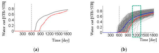
Figure 1.
Example of deterministic and stochastic approaches for assessment of reservoir uncertainty: (a) watercut from a single reservoir model (gray line) differs from the true production (red line); and (b) watercuts from one hundred reservoir models compose a band of prediction (gray lines) and cover the true production (modified from [1]).
The best way to assess the uncertainty is to perform reservoir simulation for all possible reservoir models. However, this approach is not desirable in terms of the simulation cost. The key to the assessment of reservoir uncertainty using distance-based clustering (DBC) techniques is to classify similar models as the same group. Then, we can select few representative models for each group. If we classify 800 models into ten groups and select two models for each group, 20 models are selected among all 800 possible models. The way to evaluate uncertainty using few representative models is the same as using hundreds of models. Figure 2 shows cumulative distribution function for field oil production at 1800 days. All 800 models have 800 field oil production values (the grey line) and 20 representative models have 20 field oil production values (the red line). Regardless of the number of models, uncertainty, e.g. P10, P50, and P90 or upper and lower boundaries, can be estimated. DBC enables us to replace the reservoir uncertainty obtained from hundreds or thousands of reservoir models with the uncertainty from a few representative models.
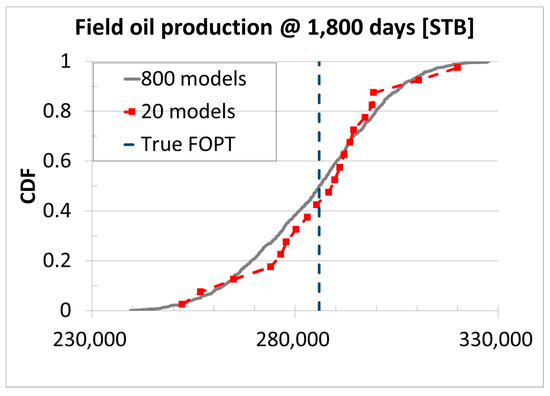
Figure 2.
Example of reservoir uncertainty analysis with all models and with representative models (modified from [2]).
The typical procedure of DBC consists of four steps: determination of a distance, construction of a matrix, dimensional reduction, and clustering (Figure 3). Distance definition is the most important step in DBC to determine the criteria for the (dis)similarity between two reservoir models (Figure 3a). Two types of distance exist: static criteria and dynamic criteria. Static distance utilizes a reservoir model itself, and dynamic distance requires additional reservoir simulation to obtain its performances. After features are defined by a distance concept, distance functions are implemented to quantify the dissimilarity between the features from two models. Here, the term of feature means main information and distinct characteristics of each reservoir model. For example, feature can be extracted by several domain transformation techniques (refer to Section 2.1). Because each pair of reservoir models has a distance value, the symmetric distance matrix can be obtained (Figure 3b). The distance matrix is converted to coordinates in a predetermined metric space by dimensional reduction algorithms to visualize the infinite dimension of the distance matrix as low dimension or extract only the core information (Figure 3c). Then, clustering algorithms are applied for points in the metric space, and each model is clustered into a specific group (Figure 3d). The representative model for each group is usually chosen by the nearest model from the center of the group members.
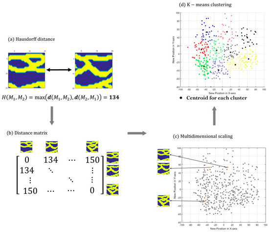
Figure 3.
Conventional workflow of DBC (modified from [3]): (a) dissimilarity between two static models is calculated by the Hausdorff distance based on the location of sand facies (yellow); (b) distance matrix consists of Hausdorff distances of model pairs; (c) relative distances are converted to coordinates by multidimensional scaling; and (d) clustering algorithms are applied to group similar models and obtain a representative model for each cluster.
The purpose of DBC can be changed depending on the availability of production data. If dynamic data are not available, the goal of DBC is to efficiently assess the reservoir uncertainty instead of reservoir simulation for hundreds of equivalent reservoir models. Therefore, DBC selects a few representative models among all reservoir models. Because the representative models are selected reasonably, their uncertainty can reproduce properly the uncertainty of all models (Figure 2). No additional information is required for DBC. If dynamic data are available, the purpose of DBC is to efficiently reduce reservoir uncertainty without complex inverse modeling algorithms. Therefore, DBC attempts to select a few qualified reservoir models, whose reservoir performances are similar to that of observed dynamic data, among all reservoir models. For further history matching, the qualified models can be coupled with data assimilation algorithms such as randomized maximum likelihood, Markov chain Monte Carlo, and ensemble Kalman filter.
The basic concept of DBC is the same but the algorithms in each step vary. Due to the scalability of DBC, various algorithms are introduced to the DBC’s four steps. This paper explains state-of-the-art DBC with features for various techniques. For better understanding, we summarized previous studies according to each step of DBC, as shown in Figure 4. The purpose of this review is to consistently analyze the scattered studies, to identify the limitations, and to suggest future study. We expect that this review paper helps to understand the DBC process and the current research trends on applying DBC in petroleum engineering.
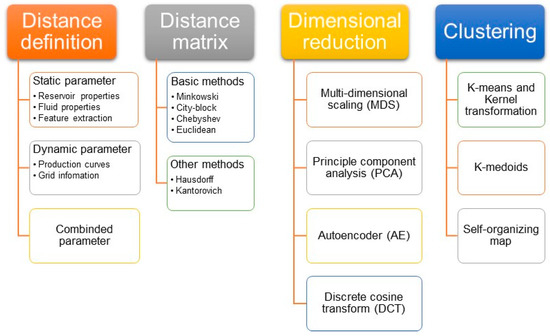
Figure 4.
Classification of typical algorithms for the four procedures in DBC.
The contents are described as followed. After the distance definition is addressed in Section 2.1, distance equations are explained in Section 2.2. Dimensional reduction methods are reviewed in Section 2.3. Three clustering algorithms and kernel transformation are discussed in Section 3.1, Section 3.2 and Section 3.3. In Section 4.1, application of DBC in real fields and unconventional cases is demonstrated, and, in Section 4.2, a synthetic case is used to compare DBC algorithms. Current DBC research is summarized, and future research trends for DBC are suggested in Section 5. Figure 4 shows the structure of the DBC procedures reviewed in this paper.
2. Distance and Dimensional Reduction
2.1. Distance
If two different facies models exist, the reservoir behaviors seem to differ (refer to Figure 5). However, evaluating quantitatively the dissimilarity between the models is another problem. To calculate a distance, a criterion for each model, which is referred to as a feature, is required. A feature can be anything if it can distinguish characteristics among different models. Previous studies have defined various distance concepts to determine dissimilarity. They can be categorized as follows:
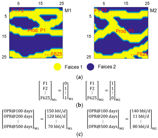
Figure 5.
Examples of distance definition (modified from [3]): (a) two facies models have a total of 625 grids and a single production well, P1; (b) facies indexes for each grid are used as the static distance; and (c) oil production rates for different time steps are used as the dynamic distance.
- Static distance
- Dynamic distance
- Combined distance
Static distance calculates a dissimilarity using reservoir property and does not require forward reservoir simulation. If any tracer or proxy simulation is used to define a distance, it is classified into a dynamic distance. Figure 5 shows an example of both static distances and dynamic distances in a 25 by 25 grid system with a single production well at the center (Figure 5a). For a simple static distance, facies codes, 1 for sand and 0 for shale, for all grids become a feature (Figure 5b). If we run a reservoir simulation for both models, monthly oil productions become dynamic distance. In Figure 5c, each model has 5 oil production rates at 100, 200, 300, 400, and 500 days. We can easily calculate summation of error between the vectors of dynamic responses from each model.
For static distance, when hundreds of reservoir models have been constructed, the reservoir properties can be compared by a grid rather than reservoir simulation for each model. While building static models, reservoir properties, such as permeability, facies, porosity, and water saturation, are assigned for each grid. Permeability is the most common reservoir property for distance definition [4,5,6,7]. It is highly correlated with future production because it is an important parameter that affects flow rate in Darcy’s law. Facies for each grid also have been applied for the criterion in many previous researches [8,9,10,11]. Facies can substantially affect the reservoir responses because parameters for a reservoir simulation, such as the relative permeability function and saturation function, are assigned according to the facies. However, these parameters have difficulty understanding spatial characteristics because they represent values in a grid.
The variogram analysis among models can confirm the relationship between the static distance and the interested reservoir performance [2,11]. The conner point grid system is used to compare the dissimilarity of structure models [12]. In an oil sands reservoir, a feature vector is defined by the shale length and the relative distance from the injection well because these parameters are important to determine steam chamber and future production [13].
Recently, multiple reservoir properties have been integrated to define static distance [14]. Facies, porosity, permeability, and water saturation for each grid are compared together using a special distance function. As more reservoir information is integrated, it may be easier to define a feature among several models. However, it can be economically and technically expensive. Therefore, some researchers suggested the average of the reservoir properties as a distance to reduce the dimension of features. Gross et al. [15] used the mean value of porosity of all grids instead of using the values of porosity of all grids themselves. That is, the information of the number of grids is reduced to one average porosity value. For example, if a 100 × 100 × 10 grid system exist, porosity information for each model consists of 100,000 values. Rather than all information, they adapt the average of 100,000 values for the feature of porosity. The researchers employed the average porosity, permeability, water saturation, and gas-in-place for a feature vector. Patel et al. [16] defined dissimilarity using statistical, fractional, and volumetric measures. They determined effective grid blocks, which can affect fluid flows, and calculated effective average properties for permeability, porosity, and irreducible-water saturation. They set a threshold value for each parameter and assigned 0 or 1 to grid blocks to comprehend whether they are effective. In addition, they measured volumetric properties such as net pore volume and original oil-in-place. These studies demonstrated that a distance can be defined by various types of static measures, which are highly related to reservoir flows and characteristics.
Several geostatistical algorithms adopted distance concepts to distinguish a subset of patterns from a training image [17,18,19,20]. They compared each grid to compute the dissimilarity of patterns. Although they applied the same criterion, i.e., index for each grid, to measure the dissimilarity of models, the result of DBC can differ due to various distance functions and clustering algorithms (refer to Section 2.2). Therefore, DBC requires overall considerations of the whole process for a successful application. Researchers should think that which function or algorithm is the most suitable for the input data used.
However, distance calculations using the static model cause the following limitations. First, the larger is the grid size, the longer is the calculation time. Second, the reliability of the dissimilarity decreases due to unnecessary information. For example, when we are concerned with the production of injected water or polymer at the production well, the reservoir properties between the injection well and the production well are key information. In other words, properties at distant grids may be unnecessary information. To resolve these limitations, a concept of feature extraction has been applied for static models to obtain core information. Some researchers applied domain transformation techniques, such as discrete Fourier transform (DFT), principal component analysis (PCA), and discrete cosine transform (DCT). Main information on channelized facies models was successfully extracted by DFT [21]. After a facies image is converted into the frequency domain by using DFT, the boundary of the image can be detected in low-frequency areas (refer to [21]). In the case of oil sands, a transformed connected hydrocarbon volume image was converted to the frequency domain by DFT to measure the dissimilarity of shale barriers [22,23]. PCA, which is a dimensional reduction technique, was applied to extract the main feature from permeability fields [24,25,26]. PCA is useful to manage high-dimensional data by obtaining the principal components of the data distribution. Because PCA can extract overall patterns in the permeability distribution, applying PCA to channel reservoirs or other types, which have distinct facies patterns, is recommended.
DCT is also used to extract the main information of a static model in a history matching area [27,28,29,30,31,32,33,34,35]. After original data are transformed to coefficients of discrete cosine functions, the coefficients are arranged in descending order of frequencies of cosine functions. Low-frequency coefficients are employed to extract essential information, such as the pattern and connectivity of a reservoir model, especially a channelized reservoir. Therefore, the number of coefficients should be chosen depending on its technical purpose.
Because the previously mentioned static distances do not require a forward simulation of a static model, definition of a distance is considerably faster than definition of dynamic distances. However, dynamic distances can provide more reliable DBC results since it is directly connected with the reservoir performance [36,37]. Many researchers utilized time-series production data, such as oil production rate, cumulative oil production, bottomhole pressure (BHP), and gas-oil ratio (GOR), as criteria of dissimilarity [7,15,38,39]. These data are easily obtained by commercial reservoir simulators. For example, saturation or pressure changes for each grid, which are calculated by reservoir simulation, are compared to calculate dissimilarity [36]. These dynamic data represent reservoir performances directly but full reservoir simulation is a burden when the reservoir is a large scale and hundreds of models exist.
Many studies have employed proxy or tracer simulations to reduce the simulation cost of forward simulation. The results of streamline simulation, such as generalized travel time, streamline density map, and oil production rates, are fast and reliable to replace conventional reservoir simulation [6,40,41,42,43,44]. A proxy model, which is built to predict specific reservoir performances, has been used to predict pseudo dynamic data, such as the water breakthrough time and monthly steam injection rate [45,46].
Some researchers used both static and dynamic features together. Average reservoir properties, such as porosity, permeability, and gas-in-place, and the sequence of dynamic data, such as the time-series pressure and production rate at the well location, are used to define the distance between reservoir models [15,47].
2.2. Distance Matrix
As previously discussed, various parameters are available to define a distance needed to determine the similarity between reservoir models. Likewise, many methods are available to calculate a distance based on static and dynamic features. Table 1 lists a group of formulas to compute the difference between two feature vectors. Because these methods are popular and known mathematical forms, we refer them as “basic methods”. These methods are used to measure the dissimilarity of data in an extensive range of research areas, which manage complex and numerous datasets, including reservoir engineering. The Euclidean distance is one of the most popular formulas because it is simple and straightforward [6,15,20,26,37,41,48,49,50,51]. It is a straight-line length between two data in Euclidean space. The Euclidean distance can be estimated in any dimensional space; thus, it is applicable to various types of data. However, it has a difficulty in understanding the overall pattern of datasets. The city-block distance is a summation of the absolute value of data misfit and is also referred to as the Manhattan distance or Taxicab geometry [18,19].

Table 1.
Mathematical formulas of a dissimilarity distance.
The Minkowski distance is a generalized form of the Euclidean distance, whose order in the equation is 2. In the formula, the order is set by any positive integer. However, an even number is recommended due to the sign problem. Figure 6 is an example of the Minkowski distance calculations with different orders: 2, 3, 4, 5, 8, and 16. A dataset consists of 12 simple channel reservoir models with different channel directions: 0 (green), 45 (blue), 90 (orange), and 135 (red) degrees. The models with the same channel directions have smaller distance values than the other reservoir models. The Minkowski distance is measured for the six orders based on facies information, i.e., static distance, for a pair of the 12 models. We denote the models as points in a 2D plane using multidimensional scaling (MDS).
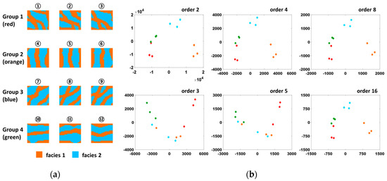
Figure 6.
Example of Minkowski distance calculation applied to 12 channel reservoir models: (a) 12 channelized reservoir models generated from four training images with different channel directions; and (b) clustering result for each order (the same dot colors represent the same group).
We draw the reservoir models in different colors according to their channel direction. A large difference in the clustering results exists between odd and even numbers for the order, although the distance definition and clustering algorithm are equivalent. In the chart, for the orders 3 and 5, the models are not reasonably grouped according to their properties. Dots in the same color should have short distances but they are mixed with other colored dots due to distortion of the sign effect during calculation. Conversely, the models are properly grouped when using with even numbers for the order. As the order is increased, the clustering results are almost similar among the graphs, with the exception of the scale.
The Chebyshev distance is another special case of the Minkowski distance, in which the order goes to positive infinity. The Chebyshev distance calculates dissimilarity using only the maximum difference among the data entries. Although calculation of the Chebyshev distance is simple, it may yield a biased value when an outlier exists in the data.
Table 2 shows distances from three different datasets, , , and , to by using various types of formula. As listed in Table 2, and are similar except for one value, i.e., an outlier at the first element in . The Chebyshev distance could be very different between case and case due to the outlier in . It is only affected by the largest outlier due to its mathematical form. Because the Euclidean, Minkowski, and City-block distances have similar equation, their calculated values show similar trends.
Table 2.
Calculation for various distances of datasets X and Y.
These calculation formulas, which we refer to as the basic methods, measure the dissimilarity by comparing grid by grid. However, when we want to examine the patterns in the data (e.g., permeability distribution patterns), these basic methods may not be useful. For this reason, some researchers applied other distance calculation methods for effective pattern recognition. One of these methods is the Hausdorff distance, which measures the distance between two datasets and enables many-to-many correspondence [3,8,9,10,11,12]. Given the two point sets A and B, the Hausdorff distance calculates the distance using Equations (1) and (2).
where is a vector norm. Because the Hausdorff distance calculates the dissimilarity of the data in a group, the distance between and in Table 2 is 0. The two point sets are identical despite different sequence. When there is an outlier as the first element of , the distance is highly affected. However, only the largest value could affect the distance calculation, case and case have the same Hausdorff distance as 6. The Hausdorff distance is useful when the dataset can be transformed into a binary set. In sandstone channel reservoirs, the models can be assumed to have two facies of sand and shale. Therefore, use of the Hausdorff distance is effective for analyzing channel reservoirs.
Pattern detection is very important in history matching analysis in channel reservoirs because oil and gas tend to flow along high permeability zones, especially sand channels. Lee and Choe (2016) [4] emphasized the importance of detecting permeability patterns and proposed a newly defined distance based on a correlation equation. However, it has a limitation of applicability in other reservoir models. Researchers tried to suggest new ideas of distance calculation, which can be applied in wide usage by changing the distance definition or combining statistical algorithms such as PCA or DCT.
Other distance calculation formulas have been employed in previous studies [14,36,39,42,52]. For example, Patel et al. [16] employed the Kantorovich distance to compare the probability distributions of the reservoir models. Their objective is to determine the reduced number of ensembles, which has the minimum difference with the original ensemble. Jin et al. [40] measured the distance by counting the number of grid blocks that are passed by streamlines to understand the flow patterns. An efficient distance matrix calculation is a very important process in DBC, because hundreds of reservoir models and hundreds of thousands of grid blocks may be employed for the analysis.
2.3. Dimensional Reduction
A single reservoir model consists of numerous grid blocks. Each grid block has unique reservoir properties, such as permeability, porosity, saturation, and pressure. Therefore, the reservoir data are usually managed in a very high-dimensional space. However, high-dimensional data reduce the calculation efficiency, and analyzing their characteristics is difficult. These limitations explain why dimensionality reduction is required for uncertainty quantification and history matching studies.
One of the most useful methods to reduce the dimension is MDS, which is a statistical method for projecting data from high spaces to low spaces. When a distance matrix is constructed for datasets, the matrix size is by . Because determining the relations within this information is difficult, we project the data onto a 2D plane. Figure 7 shows the MDS result on the 2D plane when . In Figure 7, the entries of the 3 by 3 distance matrix represent the dissimilarity between each data pair. We can easily calculate how to input the data onto the 2D space according to their distances. After fixing the two data points and in the plane, the (x,y) coordinates of the data point is obtained by Equations (3) and (4).
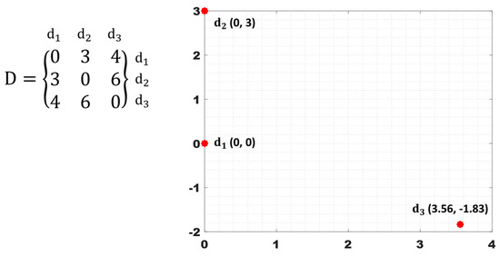
Figure 7.
Example of MDS for the three datasets.
If more than three datasets exist, an exact solution in 2D space does not exist but we numerically approximate the position. Since MDS is a simple but very powerful algorithm to manage the data, many studies used MDS to reduce the data dimension [2,3,4,6,7,8,9,14,15,18,20,21,26,36,37,38,39,40,43,44,45,51,53]. MDS can maintain the distance information while reducing the dimension in a lower space. We can reduce the dimensionality in any lower space but 2D space is the most common because critical issues do not exist to reduce to 2D and it is more suitable for data visualization than 3D.
PCA is also popular for managing high-dimensional data. PCA calculates the principal directions of data distribution from eigenvalues and eigenvectors. A covariance matrix of the data should be decomposed using eigen-decomposition or singular value decomposition. The eigenvalue indicates the degree of principal directions that correspond to its eigenvector. Because all eigenvectors are orthogonal, we can construct n-D spaces by choosing n-eigenvectors. Compared with MDS, which is only used to reduce the data dimension based on the distance information, PCA can analyze data characteristics and reduce their dimension. Therefore, PCA is extensively employed in various research areas, such as face cognition, seismic interpretation, and reservoir engineering, which require very complex calculations in high dimensions [5,24,25,42,49,50,52,54,55].
Kang and Choe [5,25] and Kang et al. [24] reduced the dimension into 2D space using PCA. Jung et al. [26] used PCA to extract the general trends of eigenvalues for efficient analyses. Because PCA is helpful for representing the data according to their main properties, it can be employed to present the data in 2D views [22,23]. There are some rules of thumb to decide the number of reduced principal components (PCs) in PCA: (1) Keep cumulative proportion of PCs at least 0.8, (2) Keep only PCs with above-average variance, (3) Keep PCs before the elbow in scree plot. Because the suitable number of PCs depends on input data or research purpose, sensitivity analysis on PCs is recommended.
Autoencoder (AE) is a data compression method based on machine learning in an unsupervised manner [2,33,56]. Figure 8 presents AE and stacked autoencoder (SAE) with an application example for a channelized reservoir. A neural network of AE is trained to show the same data in both input layer and output layer (Figure 8a). An original reservoir model is applied to the input layer and it goes through encoding. Encoded data are decoded to obtain a constructed reservoir. The neural network is modified considering discrepancy between the constructed reservoir model and the original model so that AE is learned to encode and decode. Encoding means extracting features from the input data and decoding is reconstruction of the compressed data. The number of hidden layer node is typically less than the number of node in input and output layers, AE can be used for dimension reduction.
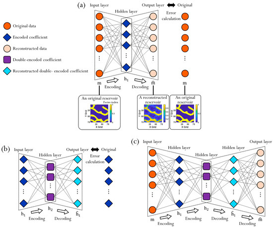
Figure 8.
Schematic diagram of autoencoder and stacked autoencoder with a channelized reservoir model [33].
Like other dimensional reduction methods, loss of information is inevitable during a dimension reduction. It is expected to mitigate critical data loss by sequential AEs rather than one AE for data compression. In Figure 8c, SAE is combination of the two AEs in Figure 8a,b. It consists of two encodings and two decodings. The inner pair of encoding and decoding are same with Figure 8b and the outer pair of encoding and decoding are came from Figure 8a. Instead of direct compression from m to , data dimension is gradually decreased to prevent from missing essential information in Figure 8c (, orange circle → , dark blue diamond → , purple square). If the dimension reduction was conducted from to right away, there could be critical data loss.
DCT has similar characteristics to DFT (discrete Fourier transform) [21] and PCA because it can extract principal properties and reduce data dimension. Especially, the basic principle of DCT and DFT is very similar. However, the difference between DCT and DFT is the type of their basis functions. In the case of DFT, given data are presented into coefficients of complex exponential functions. On the other hand, DCT utilizes cosine functions and reconstructs the given data into real-valued coefficients. When the size of the data is , the DCT function is described in Equations (5) and (6).
where is the original dataset. In addition, the coefficients can be transformed by an inverse DCT function (refer to Equation (7)) to the original data space. DCT coefficients have different information about the original data according to their frequencies. Coefficients with low frequencies have overall characteristics, while DCT functions with high frequencies represent detailed information. The selection of a subset of DCT coefficients depends on the objective of the research. For example, to characterize channel reservoirs, several papers applied DCT to permeability data to extract only the main channel trends in the ensemble models with low frequencies’ coefficients [27,28,29,30,31,32,34,35]. The channel trends in reservoirs can be described with only a small number of coefficients. How many coefficients should be kept depends on the input data used. Therefore, similar to PCA, sensitivity analysis on DCT coefficients can improve simulation efficiency. The dimension of the subset coefficients is reduced, which enables DCT to efficiently manage high-dimensional data.
3. Clustering Algorithms
Clustering algorithms, which are based on unsupervised learning theory, are powerful grouping techniques for statistical data analysis [57,58]. They assign a set of data points into a number of groups and segregate groups with similar features. Data points in the same group have similar properties or features, while data points in different groups are highly dissimilar. However, since no labels are assigned to data, clustering algorithms cannot determine which features are employed for training and grouping the data points. In addition, we often need an iterative implement of an algorithm for knowledge discovery or multiobjective optimization. Although numerous clustering algorithms exist for data mining, we present three clustering algorithms that are popular in petroleum engineering: K-means clustering, K-medoids clustering, and the self-organizing map (SOM).
3.1. K-means Clustering
K-means clustering is one of the simplest unsupervised learning algorithms [59]. The word “unsupervised” means the data are trained without knowing the known dataset. The method groups data based on their dissimilarities according to the distance [60]. The method applies the number of clusters as the input parameter and partitions a set of objects into clusters. Each cluster has a centroid, and the algorithm minimizes the defined distance between centroids and data points. A mathematics expression of the algorithm can be presented by Equation (8).
where is a binary variable, which is 1 in the case in which the th object belongs to the th cluster or 0 in the opposite case. is the distance between the th object and the centroid of the th cluster .
However, finding a global minimum of Equation (8) is difficult because the binary variable should be jointly optimized. If we want to find a global minimum, we should check all possible combinations of clusters, which has a considerably high computational cost. To solve this problem, the K-means algorithm repeats two procedures by fixing either or [8]. The Algorithm 1 consists of the following steps [61]:
| Algorithm 1 K-means clustering |
| SELECT points as the initial group centroids c1, c2, ⋯, ck |
| REPEAT |
| Make clusters by assigning data points to the closest centroid |
| Recalculate the centroid of each cluster by the mean of the data in the cluster |
| UNTIL the centroids do not change |
K-means clustering has been extensively applied to group reservoir models in petroleum engineering [13,16,45,48]. Since reservoir models usually have high dimensionality, some researchers have attempted to perform the algorithm on the featured plane using feature extraction methods, such as PCA and singular value decomposition [5,24,25]. MDS can also be utilized for dimensionality reduction of reservoir models on a 2D plane but distances between reservoir models should be predefined [3,4,6,7,8,9,21,38,53].
Although K-means clustering is fast and efficient, it cannot capture nonlinear complex patterns (Figure 9a). Kernel transformation converts data into a higher-dimensional feature space to create a more linear problem [18]. Therefore, a linear clustering technique, such as K-means clustering, can be effectively applied in the feature space (Figure 9b). When linear algorithms are applied in an infinite feature space, the kernel trick enables us to calculate distance in the feature space as a kernel function in the original space [62]. We do not know the coordinates in the feature space to calculate the distance. During K-means clustering, we have to know two types of distance: distance between two points and the distance between a point and a centroid. These distances are obtained by Equations (9) and (10). Equation (11) shows a popular kernel function—Gaussian radial basis function—and the band width can be set to 10–20% of the distance between points [63]. Note that stands for nonlinear function, which converts given data from the original space into higher feature space [42]. means kernel function and is used to calculate the distance in the feature space easily. In addition, and indicate given data.
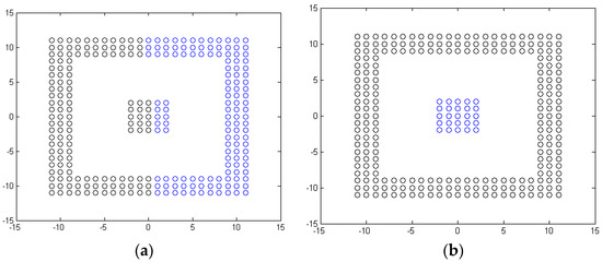
Figure 9.
Example of K-means clustering and kernel K-means clustering: (a) spherical shape results from K-means clustering; and (b) nonlinear results from kernel K-means clustering.
K-means clustering can be also utilized to define a novel clustering algorithm of spectral clustering algorithm (SCA). SCA defines a low-dimensional data space by selection of particular eigenvectors of a matrix called normalized affinity matrix, which is estimation of spatial correlation for reservoir property in each grid based on Gaussian distribution [50]. Figure 10 describes detail procedures of the SCA with an example application on a channelized reservoir model (Figure 10a). SCA builds a Gaussian affinity matrix between each pixel of the image (Figure 10b) and normalizes the matrix (Figure 10c). SCA calculates eigenvectors from the normalized matrix and selects vectors associated with the largest vectors as frequently as the number of clusters (Figure 10d). The eigenvectors are renormalized by the norm-2 of each row, and each row is regarded as each point of the reservoir model. After K-means clustering is applied for 5625 points in Figure 10e, the reservoir realization can be divided into discrete areas (Figure 10f). SCA has been utilized for many engineering areas because it is always an issue to differentiate interested physical spaces. Mouysset et al. [50] applied SCA to discretize target area that is heated by a specific heat point. Simon et al. [49] utilized SCA for categorization of an ecosystem model of the North Atlantic and Arctic Oceans. Using this SCA principle, a given image is divided into several discrete categories while retaining their geometrical features [49]. SCA is useful to understand continuously distributed natural variables such as ecological behaviors or rock type with clear boundaries so that we can make a decision in a Boolean way.
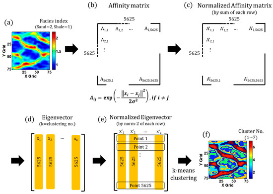
Figure 10.
Example application of SCA in a channelized reservoir model: (a) a reservoir model realization in facies index domain; (b) construction of the affinity matrix using Gaussian relationship; (c) normalization of the affinity matrix; (d) eigenvectors from the normalized affinity matrix; (e) normalization of the eigenvectors; and (f) categorization of the reservoir model using k-means clustering.
3.2. K-medoids Clustering
K-medoids clustering is similar to the K-means algorithm. Equation (8) can also explain the K-medoids algorithm. The only difference between them is the selection of centroids of clusters. In contrast to K-means clustering, centroids of K-medoids clustering primarily consist of centrally located points of clusters. Even if only one difference exists between the two methods, K-medoids clustering has advantages and disadvantages compared with K-means clustering.
First, K-medoids algorithm is substantially more robust. Since K-medoids algorithm selects centroids as the medians of each cluster, it is more protective from outliers. K-means algorithm, however, can be weak from outliers because it computes mean values to decide centroids. Second, K-medoids clustering is much more expensive, which is the main drawback compared with K-means algorithm. Since K-medoids clustering involves computing all pairwise distances to determine the centroids, its large O-notation is , whereas K-means runs in , where is the number of iterations of the algorithms. Even if the K-means algorithm is more popular in petroleum engineering research area due to its calculation efficiency, K-medoids algorithm has actively been employed for grouping models [43,64]. The detailed steps of the Algorithm 2 are listed as follows [61]:
| Algorithm 2 K-medoids clustering |
| SELECT points as the initial group medoids , , , |
| REPEAT |
| Make clusters by assigning data points to the closest medoid |
| Calculate total distance between the medoid and non-medoid data |
| FOR each medoid DO |
| Select the non-medoid to calculate new total distance |
| IF < |
| Change to |
| END IF |
| END FOR |
| UNTIL the medoids do not change |
3.3. Self-Organizing Map
The SOM is a type of competitive neural network that produces a low-dimensional (usually 2D) representation of the input data. The objects, which have similar properties in high dimension, can be classified into the same node in low dimension. As shown in Figure 11, a neural network of SOM consists of two layers, input layer and competitive layer. The network is trained to conserve the dissimilarity between objects even in low dimension.
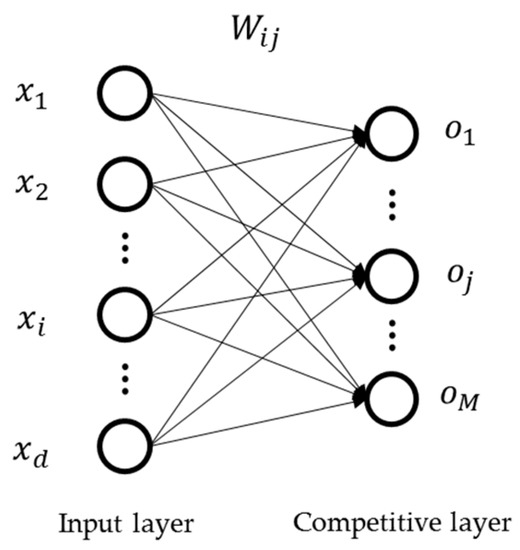
Figure 11.
A network of SOM.
where and are the th input node and the th competitive node (i.e., winning node), respectively. represents the weights that correspond to the , and the . For this architecture, we can compute the distance between the input data and the competitive node using Equation (12).
where is the distance between an input data and the th winning node. Even if the sum of square errors is generally used to calculate the dissimilarity, other distance measures can be employed. After calculating all the distances, we can decide a winning node, which has a minimum distance value. Then, we only update the weights of a winning node by Equation (13).
where subscript means the winning node. and are the weights between the and the winning node, before update and after update, respectively. is a learning rate.
Since every input object can be classified into a competitive node, it is a kind of clustering algorithm [17,22,65]. Even if various input data can be grouped into the same winning node, the distances between data and the winning node should differ. Using the distances, we can present whole data into low-dimensional space. Consequently, the SOM is a method of dimensionality reduction.
All clustering techniques, including K-means, K-medoids, and SOM, have difficulty in determining the appropriate number of clusters. Recently, there are various novel methods to automatically set the number of clusters: silhouette index, elbow criterion, cluster validity index, and Calinski–Harabasz index [20,39,46,47,66].
4. Applications
4.1. Unconventional Resources and Real Fields
With a decade of development, DBC has been verified not only for synthetic cases but also for real fields and benchmark fields. There are many applications of DBC in unconventional resources, such as oil sands, and in enhanced oil recovery (EOR) screening. DBC can be effectively applied to these areas because more time is required to implement a reservoir simulation for oil sands and EOR cases. For these cases, predicting reliable reservoir performances is difficult due to the complexity and uncertainty in a production mechanism. Especially, the combined case, EOR for unconventional resources, requires more considerations such as molecular diffusion, nanopore effect, and adsorption effect [67]. In the case of oil sands, uncertainty in shale barriers, which have a considerable impact on oil production, has been investigated. In the case of EOR, DBC is used to construct a proposal system for a suitable EOR method.
Reservoir simulation cost for unconventional resources is higher than conventional resources due to a complex production mechanism, e.g., thermal method for oil sands, hydraulic fracturing for shale, and a depressure method for coalbed methane. The difficulties in predicting shale production are well explained in [68,69,70]. As shown in the above papers, production mechanisms between conventional and unconventional resources are quite different in the case of physical-based forward simulation. However, there is no problem for DBC to apply to unconventional resources considering the four steps in DBC because DBC starts with extraction of feature of reservoir models, not complex reservoir model itself. It is a key issue to set a distance definition properly for target unconventional resources, e.g., the location of shale barrier for oil sands. In this condition, reducing the number of reservoir simulations by DBC will be more effective in unconventional resources than conventional resources.
The production of oil sands via steam-assisted gravity drainage is highly correlated to the extension of a steam chamber. The steam injected through the upper injection well lowers the viscosity of bitumen. Interbedded shale acts as a barrier to steam expansion and adversely affects productivity. Therefore, features related to shale barriers can be employed to measure the dissimilarity between two oil sands reservoirs. Connected hydrocarbon volume is applied in not only DBC but also ranking methods [22,23,71]. Figure 12a shows the concept of connected hydrocarbon volume (grey area). The black and white colors indicate sand and shale facies and the red circle means steam injection well. Connected hydrocarbon volume can be defined by the straight line from the injection well until it meets the shale facies. The grey area can be expressed as a polar coordinate system, in which the steam spreads from a well location (Figure 12b). The polar coordinate system has the effect of weighting on shale barrier near the wells. Key information, which was extracted via DFT, was defined as the distance (Figure 12c). This study, however, assumed that steam could not detour the shale barriers and would extend to a 180 degree radius. To overcome this limitation, the steam is spread within a 90 degree radius and bypassed in the form of a triangle when it encounters shale barrier [13]. These techniques used static distances that do not require dynamic simulation. Another study defined dynamic distance by streamline simulation. The distance between the models is defined by setting the streamline map as a feature. Although additional simulation time is required, it is minimized by streamline simulation. Simulating steam expansion more realistically than the previous methods is advantageous [38].
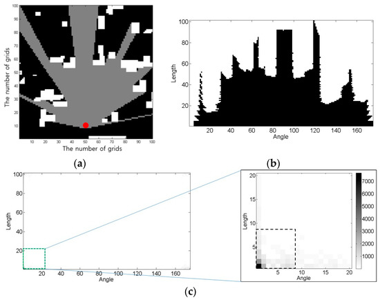
Figure 12.
Feature extraction using connected hydrocarbon volume (the grey area) concept in oil sands reservoirs (modified from [23]): (a) straight lines from the injection well (the red circle) until they meet shale facies (the white area); (b) the sight map is converted into a polar coordinate system, which has an x-axis and y-axis that is represented as the angle and the length, respectively; and (c) few parameters in the frequency domain by DFT are used for a feature.
Recently, some researchers have attempted to define a feature for oil sands according to well production data from full reservoir simulations [39,46]. Information for a well pair, oil production rates for a production well and the steam injection rate for the injection well were employed to calculate the dissimilarities for a thousand of 2D synthetic models [39]. They employed MDS two times to exclude redundant models among the 1000 models for effective clustering. Other researchers developed a proxy model by an artificial neural network to determine the location of the shale barrier by history matching [46]. The model can predict oil production according to the location of a shale barrier in oil sands reservoirs. To verify the performance of the proposed method, DBC is used to characterize the models. Eight hundred oil sands reservoirs are classified into two categories based on the presence of shale barriers between the injection well and the production well. Steam injection rate was defined as a feature vector and K-means clustering was directly applied to a 10-dimensional metric space without distance calculation and dimension reduction procedures. However, these two studies are applied only to 2D synthetic oil sands fields.
Some researchers have attempted to extend their idea to 3D synthetic cases before applying to benchmark or real fields but the number of grids and generality remain limited [9,14,36]. Benchmark fields, such as PUNQ-S3 field, can be used to test a novel method to obtain field applicability [6,24,25]. The grid system of PUNQ-S3 consists of 19 by 28 by 5, and the first, third, and fifth layers have similar high permeability tendencies in the southeast direction. Six production wells and oil production rates, BHP, GOR, and watercut are observed for each well. Because GOR is the most sensitive parameter among the dynamic responses, it was employed for a distance criterion [7]. After the Minkowski distance was applied to GOR, MDS and K-means clustering are utilized. In the same paper, horizontal permeability was also tested to define a dissimilarity as static distance. Permeabilities in a total of 1761 active grids became a feature vector and the same procedure—the Minkowski, MDS, and K-means clustering—was utilized. The only difference was the distance definition for PUNQ-S3 model: 6 GORs and 1761 permeabilities. Other cases applied the concept of feature extraction for PUNQ-S3 [24,25]. Two features were extracted by PCA, and 400 models were marked in 2D metric space. K-means clustering was directly applied without a dimension reduction technique. This DBC showed better sampling performance than random sampling. Although it takes times for DBC, simulation results are more reliable and time-efficient.
DBC has been verified via the following real field cases. An offshore turbidite reservoir in West Africa was utilized for uncertainty quantification by dynamic distances [37]. The field model consists of 78 by 59 by 116, which is more than 100,000 active grids, 28 wells, 20 production wells and 8 injection wells. Due to the geological uncertainty in the facies concept and the proportion, a total of 72 possible models were generated by 12 training images and three scenarios of facies ratios (two realizations for 36 combinations). After a streamline simulation was implemented for the whole models, cumulative oil and water productions were applied for the dissimilarity calculation. Late responses were utilized instead of the early production data because the dissimilarity between the two models is easily characterized after the water breakthrough. A 72 by 72 distance matrix was converted into 2D coordinates, and kernel K-means was applied to select seven representative models. After implementing numerical simulation, uncertainty range, e.g. P10, P50, and P90, for cumulative oil production from the representative models successfully mimic the uncertainty from the 72 models. This flow-based distance secured greater accuracy over the static distance, which provides more generality solutions than the dynamic distance [37].
DBC is useful for determining field development plan considering the uncertainty in the reservoir model. Gross et al. [15] applied DBC to an offshore gas field, which has two major anticline structures. The first structure has been already developed with five production wells since 2001 and they want to extend the field boundary to the second structure. They used DBC to handle the uncertainty in linkage of the two anticlines to determine field development plan. The eight representative models are selected among 925 possible models by DBC [15]. The eight models are tested for 28 candidates of field development instead of the 925 models. In this paper, three distance concepts were tested: static distance only, dynamic distance only, and combination of static and dynamic distances. For static distance, 12 average static properties for three regions were employed: porosity, permeability, water saturation, and gas-in-place. After comparing the normalized feature vector from each model by the Euclidean distance, MDS and K-means clustering are applied in order. For dynamic distance, 11 variables for five wells were applied: BHP, flow rate for each well, and cumulative gas production. The dimension of the dynamic feature vector is considerably higher than 11 due to several time steps. In this case, kernel transformation was applied for better K-means clustering results. A weighted distance of the two distances was tested for the combined case. In this paper, more weighting is given for the static distance than the dynamic distance due to the early stage of the field development. Conditions for a reservoir simulation used to obtain dynamic distance can be changed according to the development schedule.
Because the EOR process requires a complex reservoir simulation that is related to chemical or thermal behaviors in a reservoir, a proxy model and DBC are more powerful solution for uncertainty quantification. In the case of polymer flooding, a 2D synthetic case [45] and 3D real field case [43] were investigated. For the synthetic case, two dynamic features of recovery factor and water breakthrough were used to distinguish 600 channelized models [45]. To reduce the simulation cost of flow-based distance, the recovery factor and water breakthrough are calculated by a material balance and a proxy model, respectively. Although it is a complex EOR problem, the same DBC procedure of the water flooding case can be applied to this problem because the connectivity of injection and production wells is important for reservoir behavior. For the real field case, DBC is employed to determine the location of a polymer injection well [43]. After a polymer pilot is successfully applied for the 8 TH reservoir in Matzen Field in the Vienna basin, the second injection well is planned for the extension of the pilot. Eight hundred reservoir models, which has 658,560 active cells with four facies, are generated with various variogram models to consider the geological uncertainty. Using streamline simulation, the tracer concentration at the production wells, which is highly correlated to the connectivity between the injection well and the production well, is obtained. After applying MDS and K-medoids clustering, 70 selected models among the 800 models are used to predict future performances by full reservoir simulation.
In the case of low salinity water flooding, a chemical module should be carefully selected by screening depending on the reservoir and fluid properties. The criterion of EOR screening is usually determined by previous EOR projects. Some researchers have classified the conditions of EOR projects to develop a decision-making system for a proper EOR method [47,52]. In [47], after 151 EOR projects were reviewed, the following nine variables were applied for a feature vector: four rock properties (permeability, porosity, reservoir depth, and thickness) and five fluid properties (oil saturation, gravity, temperature, viscosity, and pressure). Without a dimension reduction technique, a fuzzy C-means clustering algorithm was used to minimize the impact on outliers. The number of clusters was determined to be three by a cluster validity index. If a new EOR project is examined, it can propose a proper EOR method according to the closest group.
Siena et al. [52] also considered various reservoir properties for discrimination criteria: density, viscosity, porosity, permeability, depth, and temperature. They reduced the dimensionality of the parameter space by PCA and measured the similarity between EOR projects. Additionally, they utilized a Bayesian-clustering algorithm to assess the analogy between a preprocessed dataset and the target data based on the reservoir parameters. The proposed method showed the applicability for planning and assessing the EOR projects when it is applied to the real field operated by Eni.
4.2. Comparisons of a Synthetic Case
As discussed above, many methods are available to measure the dissimilarity using different reservoir properties and mathematical formulas. Considering reservoir characteristics such as lithology or fluid phases, a suitable distance definition should be established for successful clustering analysis. Although determining the best distance calculation is challenging, we perform a comparison of the clustering results on a synthetic channel reservoir. The results may be helpful as a guideline to choose a proper distance.
Figure 13 shows DBC results using the four distance equations in Table 1. The 12 models in Figure 6a are reused. The models have different channel directions, and each model has two different rock facies: sand and shale. We expect the reservoir models to be properly categorized when we utilize proper clustering methods. We consider whether different reservoir models are represented far from one another onto a 2D plane. The channel directions are perpendicular to each other between Group 1 and Group 3 and between Group 2 and Group 4. Therefore, Groups 1 and 3 (or Groups 2 and 4) are supposed to be indicated with a far distance from each other.
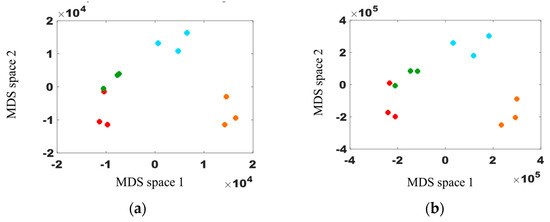
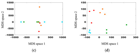
Figure 13.
DBC with the four distance equations: (a) Euclidean; (b) City-block; (c) Chebyshev; and (d) Hausdorff.
Figure 13a provides reliable clustering results from the definition of the Euclidean distance. The same result is obtained when the order is equal to 2 in Figure 6b. The dots on Figure 13a are distributed in an anticlockwise direction from the red dots to the green dots, while the channel direction changes clockwise. This finding indicates that the consistency of clustering corresponds to a channel direction with the Euclidean distance. Figure 13b uses the City-block distance instead of the Euclidean distance. As shown in Figure 13b, the overall clustering trend is similar to the Euclidean result, although the City-block distance values may differ from the Euclidean distance. Note that Figure 13b has a larger scale than Figure 13a due to different distance calculations. Although we employ a few models, the two distances can produce different results, especially complex real models.
The Chebyshev distance is utilized in Figure 13c, and the clustering result is not reasonable compared with the previous two results. Although the clustering trend has some patterns, the models are mixed up and overlapped because the Chebyshev primarily reflects the max difference and disregards other information. The Hausdorff distance presents a better clustering result than the Chebyshev distance (Figure 13d). The distribution of the dots differs from those of the Euclidean and City-block distances due to different distance definitions. The green and red dots are overlapped in Figure 13a,b, but they are classified in Figure 13d.
5. Conclusions
This paper reviews DBC algorithms and demonstrates their applications in various reservoirs for uncertainty assessment. The distance can be defined by any reservoir information if it explains the reservoir characteristics and production performances. Many papers have proposed new ideas about matrix construction and clustering techniques for an efficient analysis. However, most of these algorithms are not new and they have been employed in other research areas. Therefore, adopting ideas and technical schemes from other studies is recommended for efficient assessment of reservoir uncertainty by DBC due to its scalability.
DBC is a combination of the four technical processes: distance definition, distance matrix construction, dimensional reduction, and clustering. It is important that overall concerns on these four steps should be considered together to propose a new idea of DBC scheme. Researchers should construct DBC process, considering characteristics and limitation of algorithms. For example, the Hausdorff distance can be used only in binary data. If there are some outliers in input data, K-means clustering is not a suitable option. Instead, K-medoids clustering or other schemes would be a better choice.
For future DBC studies, machine learning is expected to be promising. Because the distance definition is critical to the result of DBC, machine learning methods such as K-singular values decomposition and AE can be applied to extract features. Deep learning such as a convolutional neural network is useful to learn essential information from complicated data. In addition, machine learning algorithm such as support vector machine can be used to group the similar models in the metric space instead of clustering techniques. There are several clustering schemes that can be applied in reservoir engineering study such as agglomerative hierarchical clustering, expectation-maximization clustering using Gaussian mixture models, fuzzy clustering, and density-based spatial clustering of application with noise. Because these methods are useful to classify the data, they are expected to be used for distance-based analysis. In the case of neural network algorithms, features in input layers are determined by PCA analysis and clustering algorithms are employed for training data set to build a reliable neural network for each cluster separately. Related to pattern detection, convolution neural network can be used to extract feature and compare reservoir models. Therefore, we need to consider a variety of applications of machine learning methods to improve reliability of DBC. In addition, DBC can be applied to other research areas related to managing high dimensional data such as face recognition, pattern search, and sales marketing.
Since the applicability of the synthetic fields has been verified by previous researches, field applications seem to be more important in future research. For unconventional resources, uncertainty assessments of stimulated reservoir volume for shale resources and uncertainty assessments of shale barriers in oil sands can be important research topics. In addition, DBC can be coupled with various techniques, such as feature extraction, distance calculation function, dimension reduction and kernel transformation, and clustering algorithm. Therefore, it is important to use an optimal DBC by considering the characteristics of each technique and model parameters in each technique.
Author Contributions
B.K. investigated several mathematical algorithms, such as distance matrix calculation and dimension reduction, implemented synthetic case, and summarized the manuscript in the Conclusion Section. S.K. reviewed the synthetic case results and suggested future research in the Conclusion Section. K.L. identified the outline of the paper with the Abstract and Introduction and described the distance definition, kernel transformation, and field applications. H.J. reviewed the clustering algorithms. J.C. participated in the writing of the manuscript and its revision.
Funding
This study was supported by the project of Korea Institute of Geoscience and Mineral Resources (KIGAM) (GP2017-024) and the project of Korea Institute of Energy Technology Evaluation and Planning (KETEP) granted financial resource from the Ministry of Trade, Industry and Energy (MOTIE), Republic of Korea (No. 20172510102090). In addition, this research was supported by Global Ph.D. Fellowship Program through the National Research Foundation of Korea (NRF) funded by the Ministry of Education (2015H1A2A1030756).
Acknowledgments
This study was supported by the project of Korea Institute of Geoscience and Mineral Resources (KIGAM) (GP2017-024) and the project of Korea Institute of Energy Technology Evaluation and Planning (KETEP) granted financial resource from the Ministry of Trade, Industry and Energy (MOTIE), Republic of Korea (No. 20172510102090). In addition, this research was supported by Global Ph.D. Fellowship Program through the National Research Foundation of Korea (NRF) funded by the Ministry of Education (2015H1A2A1030756). The authors also thank The Institute of Engineering Research at Seoul National University, Korea.
Conflicts of Interest
The authors declare no conflict of interest.
References
- Lee, K. Channelized Reservoir Characterization using Ensemble Smoother with a Distance-Based Method. PhD Thesis, Seoul National University, Seoul, Korea, 2014. [Google Scholar]
- Lee, K.; Lim, J.; Ahn, S.; Kim, J. Feature extraction using a deep learning algorithm for uncertainty quantification of channelized reservoirs. J. Pet. Sci. Eng. 2018, 171, 1007–1022. [Google Scholar] [CrossRef]
- Lee, K.; Lim, J.; Choe, J.; Lee, H.S. Regeneration of channelized reservoirs using history-matched facies-probability map without inverse scheme. J. Pet. Sci. Eng. 2017, 149, 340–350. [Google Scholar] [CrossRef]
- Lee, J.; Choe, J. Reliable reservoir characterization and history matching using a pattern recognition based distance. In Proceedings of the ASME 2016 35th International Conference on Ocean, Offshore and Arctic Engineering, Busan, Korea, 19–24 June 2016. [Google Scholar]
- Kang, B.; Choe, J. Regeneration of initial ensembles with facies analysis for efficient history matching. J. Energy Resour-ASME 2017, 139, 042903. [Google Scholar] [CrossRef]
- Kang, B.; Choi, J.; Lee, K.; Jang, I.; Choe, J. Distance-based clustering using streamline simulations for efficient uncertainty assessment. In Proceedings of the 18th Annual Conference of IAMG, Perth, Australia, 2–9 September 2017. [Google Scholar]
- Lee, K.; Jung, S.; Lee, T.; Choe, J. Use of clustered covariance and selective measurement data in ensemble smoother for three-dimensional reservoir characterization. J. Energy Resour-ASME 2017, 139, 022905. [Google Scholar] [CrossRef]
- Lee, K.; Jeong, H.; Jung, S.; Choe, J. Characterization of channelized reservoir using ensemble Kalman filter with clustered covariance. Energy Explor. Exploit. 2013, 31, 17–29. [Google Scholar] [CrossRef]
- Lee, K.; Jung, S.; Choe, J. Ensemble smoother with clustered covariance for 3D channelized reservoirs with geological uncertainty. J. Pet. Sci. Eng. 2016, 145, 423–435. [Google Scholar] [CrossRef]
- Suzuki, S.; Caers, J. A distance-based prior model parameterization for constraining solutions of spatial inverse problems. Math. Geosci. 2008, 40, 445–469. [Google Scholar] [CrossRef]
- Suzuki, S.; Caers, J. History matching with an uncertain geological scenario. In Proceedings of the SPE Annual Technical Conference and Exhibition, San Antonio, TX, USA, 24–27 September 2006. [Google Scholar]
- Suzuki, S.; Caumon, G.; Caers, J. Dynamic data integration for structural modeling: Model screening approach using a distance-based model parameterization. Computat. Geosci. 2008, 12, 105–119. [Google Scholar] [CrossRef]
- Lee, H.; Jin, J.; Shin, H.; Choe, J. Efficient prediction of SAGD productions using static factor clustering. J. Energy Resour-ASME 2015, 137, 032907. [Google Scholar] [CrossRef]
- Sahaf, Z.; Hamdi, H.; Mota, R.C.R.; Sousa, M.C.; Maurer, F. A Visual Analytics Framework for Exploring Uncertainties in Reservoir Models. In Proceedings of the 13th International Joint Conference on Computer Vision, Madeira, Portugal, 27–29 January 2018. [Google Scholar] [CrossRef]
- Gross, H.; Honarkhah, M.; Chen, Y. Offshore Gas Condensate Field History-Match and Predictions: Ensuring Probabilistic Forecasts Are Built with Diversity in Mind. In Proceedings of the SPE Asia Pacific Oil and Gas Conference and Exhibition, Jakarta, Indonesia, 20–22 September 2011. [Google Scholar] [CrossRef]
- Patel, R.G.; Trivedi, J.; Rahim, S.; Li, Z. Initial sampling of ensemble for steam-assisted-gravity-drainage-reservoir history matching. SPE J. 2015, 54, 424–441. [Google Scholar] [CrossRef]
- Li, Q.; Aguilera, R. Unsupervised Statistical Learning with Integrated Pattern-Based Geostatistical Simulation. In Proceedings of the SPE Western Regional Meeting, Garden Grove, CA, USA, 22–26 April 2018. [Google Scholar]
- Honarkhah, M.; Caers, J. Stochastic simulation of patterns using distance-based pattern modeling. Math. Geosci. 2010, 42, 487–517. [Google Scholar] [CrossRef]
- Arpat, G.B.; Caers, J. A Multiple-scale, Pattern-based Approach to Sequential Simulation. In Quantitative Geology and Geostatistics: Proceedings of the 7th International Geostatistics Congress, Banff, AB, Canada, 2004; Springer: Dordrecht, The Netherlands, 2005; Volume 14. [Google Scholar] [CrossRef]
- Koneshloo, M.; Aryana, S.A.; Grana, D.; Pierre, J.W. A workflow for static reservoir modeling guided by seismic data in a fluvial system. Math. Geosci. 2017, 49, 995–1020. [Google Scholar] [CrossRef]
- Lee, K.; Jeong, H.; Jung, S.; Choe, J. Improvement of ensemble smoother with clustering covariance for channelized reservoirs. Energy Explor. Exploit. 2013, 31, 713–726. [Google Scholar] [CrossRef]
- Lim, J.; Jin, J.; Choe, J. Features Modeling of Oil Sands Reservoirs in Metric Space. Energy Source Part A 2014, 36, 2725–2735. [Google Scholar] [CrossRef]
- Lim, J.; Jin, J.; Lee, H.; Choe, J. Uncertainty Analysis of Oil Sands Reservoirs Using Features in Metric Space. Energy Source Part A 2015, 37, 1736–1746. [Google Scholar] [CrossRef]
- Kang, B.; Yang, H.; Lee, K.; Choe, J. Ensemble Kalman filter with principal component analysis assisted sampling for channelized reservoir characterization. J. Energy Resour-ASME 2017, 139, 032907. [Google Scholar] [CrossRef]
- Kang, B.; Choe, J. Initial model selection for efficient history matching of channel reservoirs using ensemble smoother. J. Pet. Sci. Eng. 2017, 152, 294–308. [Google Scholar] [CrossRef]
- Jung, H.; Jo, H.; Kim, S.; Lee, K.; Choe, J. Geological model sampling using PCA-assisted support vector machine for reliable channel reservoir characterization. J. Pet. Sci. Eng. 2018, 167, 396–405. [Google Scholar] [CrossRef]
- Jafarpour, B.; McLaughlin, D.B. History matching with an ensemble Kalman filter and discrete cosine parameterization. Comput. Geosci. 2008, 12, 227–244. [Google Scholar] [CrossRef]
- Jafarpour, B.; McLaughlin, D.B. Reservoir Characterization With the Discrete Cosine Transform. SPE J. 2009, 14, 181–202. [Google Scholar] [CrossRef]
- Zhao, Y.; Forouzanfar, F.; Reynolds, A.C. History matching of multi-facies channelized reservoirs using ES-MDA with common basis DCT. Comput. Geosci. 2017, 21, 1343–1364. [Google Scholar] [CrossRef]
- Kim, S.; Lee, C.; Lee, K.; Choe, J. Characterization of channel oil reservoirs with an aquifer using EnKF, DCT, and PFR. Energy Explor. Exploit. 2016, 34, 828–843. [Google Scholar] [CrossRef]
- Kim, S.; Lee, C.; Lee, K.; Choe, J. Characterization of channelized gas reservoirs using ensemble Kalman filter with application of discrete cosine transformation. Energy Explor. Exploit. 2016, 34, 319–336. [Google Scholar] [CrossRef]
- Kim, S.; Min, B.; Lee, K.; Jeong, H. Integration of an Iterative Update of Sparse Geologic Dictionaries with ES-MDA for History Matching of Channelized Reservoirs. Geofluids 2018, 2018, 1532868. [Google Scholar] [CrossRef]
- Kim, S.; Min, B.; Kwon, S.; Chu, M. History Matching of a Channelized Reservoir Using a Serial Denoising Autoencoder Integrated with ES-MDA. Geofluids 2019, 2019. [Google Scholar] [CrossRef]
- Jo, H.; Jung, H.; Ahn, J.; Lee, K.; Choe, J. History matching of channel reservoirs using ensemble Kalman filter with continuous update of channel information. Energy Explor. Exploit. 2017, 35, 3–23. [Google Scholar] [CrossRef]
- Jung, H.; Jo, H.; Kim, S.; Lee, K.; Choe, J. Recursive update of channel information for reliable history matching of channel reservoirs using EnKF with DCT. J. Pet. Sci. Eng. 2017, 154, 19–37. [Google Scholar] [CrossRef]
- Insuasty, E.; Van den Hof, P.M.; Weiland, S.; Jansen, J.D. Flow-based dissimilarity measures for reservoir models: A spatial-temporal tensor approach. Comput. Geosci. 2017, 21, 645–663. [Google Scholar] [CrossRef]
- Scheidt, C.; Caers, J. Uncertainty quantification in reservoir performance using distances and kernel methods—Application to a west africa deepwater turbidite reservoir. SPE J. 2009, 14, 680–692. [Google Scholar] [CrossRef]
- Lee, K.; Jo, G.; Choe, J. Improvement of ensemble Kalman filter for improper initial ensembles. Geosyst. Eng. 2011, 14, 79–84. [Google Scholar] [CrossRef]
- Zheng, J.; Leung, J.Y.; Sawatzky, R.P.; Alvarez, J.M. A Cluster-Based Approach for Visualizing and Quantifying the Uncertainty in the Impacts of Uncertain Shale Barrier Configurations on SAGD Production. In Proceedings of the SPE Canada Heavy Oil Technical Conference, Calgary, AB, Canada, 13–14 March 2018. [Google Scholar]
- Jin, J.; Lim, J.; Lee, H.; Choe, J. Metric space mapping of oil sands reservoirs using streamline simulation. Geosyst. Eng. 2011, 14, 109–113. [Google Scholar] [CrossRef]
- Park, K.; Caers, J. History matching in low-dimensional connectivity-vector space. In Proceedings of the EAGE Conference on Petroleum Geostatistics, Cascais, Portugal, 10–14 September 2007. [Google Scholar]
- Scheidt, C.; Caers, J. Representing Spatial Uncertainty Using Distances and Kernels. Math. Geosci. 2009, 41, 397. [Google Scholar] [CrossRef]
- Chiotoroiu, M.M.; Peisker, J.; Clemens, T.; Thiele, M.R. Forecasting Incremental Oil Production of a Polymer-Pilot Extension in the Matzen Field Including Quantitative Uncertainty Assessment. SPE Reserv. Eval. Eng. 2017, 20, 894–905. [Google Scholar] [CrossRef]
- Caers, J.; Park, K. A distance-based representation of reservoir uncertainty: The metric EnKF. In Proceedings of the ECMOR XI-11th European Conference on the Mathematics of Oil Recovery, Bergen, Norway, 8–11 September 2008. [Google Scholar]
- Srinivasan, S.; Mantilla, C. Uncertainty Quantification and Feedback Control Using a Model Selection Approach Applied to a Polymer Flooding Process. In Proceedings of the Geostatistics, Oslo, Norway, 11–15 June 2012. [Google Scholar]
- Zheng, J.; Leung, J.Y.; Sawatzky, R.P.; Alvarez, J.M. An AI-based workflow for estimating shale barrier configurations from SAGD production histories. Neural Comput. Appl. 2018. [Google Scholar] [CrossRef]
- Khojastehmehr, M.; Naderifar, A.; Aminshahidy, B. Enhanced oil recovery assignment using a new strategy for clustering oil reservoirs: Application of fuzzy logics. J. Chemometr. 2018. [Google Scholar] [CrossRef]
- Park, J.; Jin, J.; Choe, J. Uncertainty quantification using streamline based inversion and distance based clustering. J. Energy Resour-ASME 2016, 138, 012906. [Google Scholar] [CrossRef]
- Simon, E.; Samuelsen, A.; Bertino, L.; Mouysset, S. Experiences in multiyear combined state-parameter estimation with an ecosystem model of the North Altlantic and Artic Oceans using the Ensemble Kalman Filter. J. Mar. Syst. 2015, 152, 1–17. [Google Scholar] [CrossRef]
- Mouysset, S.; Noailles, J.; Ruiz, D. On An Interpretation of Spectral Clustering Via Heat Equation And Finite Elements Theory. In Proceedings of the WCE (World Congress on Engineering), London, UK, 30 June–2 July 2010. [Google Scholar]
- Lee, K.; Kim, S.; Choe, J.; Min, B.; Lee, H.S. Iterative static modeling of channelized reservoirs using history-matched facies probability data and rejection of training image. Pet. Sci. 2019, 16, 127–147. [Google Scholar] [CrossRef]
- Siena, M.; Guadagnini, A.; Della Rossa, E.; Lamberti, A.; Masserano, F.; Rotondi, M. A Novel Enhanced-Oil-Recovery Screening Approach Based on Bayesian Clustering and Principal-Component Analysis. SPE J. 2016, 19, 382–390. [Google Scholar] [CrossRef]
- Kang, B.; Jung, H.; Choi, J.; Choe, J. Improvement of Simulation Runs Using Clustering Schemes in Generalized Travel Time Inversion. In Proceedings of the 18th Annual Conference of IAMG, Perth, Australia, 2–9 September 2017. [Google Scholar]
- Chen, C.; Gao, G.; Ramirez, B.A.; Vink, J.C.; Girardi, A.M. Assisted History Matching of Channelized Models Using Pluri-Principal Component Analysis. SPE J. 2016, 21, 1793–1812. [Google Scholar] [CrossRef]
- Amirian, E.; Leung, J.Y.; Zanon, S.; Dzurman, P. Integrated cluster analysis and artificial neural network modeling for steam-assisted gravity drainage performance prediction in heterogeneous reservoirs. Expert Syst. Appl. 2015, 42, 723–740. [Google Scholar] [CrossRef]
- Canchumuni, S.A.; Emerick, A.A.; Pacheco, M.A. Integration of ensemble data assimilation and deep learning for history matching facies models. In Proceedings of the Offshore Technology Conference, Rio de Janeiro, Brazil, 24–26 October 2017. [Google Scholar]
- Jain, A.K.; Murty, M.N.; Flynn, P.J. Data clustering: A review. ACM Comput. Surv. 1999, 31, 264–323. [Google Scholar] [CrossRef]
- Rojas, T.; Demyanov, V.; Christie, M.; Arnold, D. Learning uncertainty from training images for reservoir predictions. In Mathematics of Planet Earth; Pardo-Igúzquiza, E., Guardiola-Albert, C., Heredia, J., Moreno-Merino, L., Durán, J., Vargas-Guzmán, J., Eds.; Springer: Berlin/Heidelberg, Germany, 2014; pp. 147–151. [Google Scholar]
- Velmurugan, T.; Santhanam, T. Computational complexity between K-means and K-medoids clustering algorithms for normal and uniform distributions of data points. J. Comp. Sci. 2010, 6, 363–368. [Google Scholar] [CrossRef]
- Arora, P.; Deepali; Varshney, S. Analysis of K-means and K-medoids algorithm for big data. In Proceedings of the International Conference on Information Security & Privacy, Nagpur, India, 11–12 December 2015. [Google Scholar]
- Patel, A.; Singh, P. New approach for K-mean and K-medoids algorithm. IJCAES 2013, 2, 1–5. [Google Scholar] [CrossRef]
- Shawe-Taylor, J.; Cristianini, N. Kernel Methods for Pattern Analysis; Cambridge University Press: Cambridge, UK, 2004. [Google Scholar]
- Shi, J.; Malik, J. Normalized cuts and image segmentation. IEEE Trans. Pattern Anal. Mach. Intell. 2000, 22, 888–905. [Google Scholar] [CrossRef]
- Hingerl, F.F.; Thiele, M.R.; Batycky, R.P. Reservoir Management of a Low-Salinity Flood on a Per-Pattern Basis. In Proceedings of the SPE Improved Oil Recovery Conference, Tulsa, OK, USA, 14–18 April 2018. [Google Scholar] [CrossRef]
- Kharyba, E.; Demyanov, V.; Antropov, A.; Malencic, L.; Stulov, L. Neural network classification to improve geological and engineering understanding for more reliable reservoir prediction. In Proceedings of the 19th Annual Conference of the International Association for Mathematical Geosciences, Olomouc, Czech Republic, 2–8 September 2018. [Google Scholar]
- Milligan, G.W.; Cooper, M.C. An examination of procedures for determining the number of clusters in a data set. Psychometrika 1985, 50, 159–179. [Google Scholar] [CrossRef]
- Jia, B.; Tsau, J.-S.; Barati, R. A review of the current progress of CO2 injection EOR and carbon storage in shale oil reservoirs. Fuel 2019, 236, 404–427. [Google Scholar] [CrossRef]
- Alharthy, N.; Teklu, T.W.; Kazemi, H.; Graves, R.M.; Hawthorne, S.B.; Braunberger, J.; Kurtoglu, B. Enhanced Oil Recovery in Liquid-Rich Shale Reservoirs: Laboratory to Field. SPE Reserv. Eval. Eng. 2018, 21, 137–159. [Google Scholar] [CrossRef]
- Jia, B.; Tsau, J.-S.; Barati, R. Measurement of CO2 Diffusion Coefficient in the Oil-Saturated Porous Media. In Proceedings of the Abu Dhabi International Petroleum Exhibition and Conference, Abu Dhabu, UAE, 12–15 November 2018. [Google Scholar] [CrossRef]
- Jia, B.; Tsau, J.-S.; Barati, R. Role of molecular diffusion in heterogeneous, naturally fractured shale reservoirs during CO2 huff-n-puff. J. Pet. Sci. Eng. 2018, 164, 31–42. [Google Scholar] [CrossRef]
- Fenik, D.R.; Nouri, A.; Deutsch, C.V. Criteria for ranking realizations in the investigation of SAGD reservoir performance. In Proceedings of the Canadian International Petroleum Conference, Calgary, AB, Canada, 16–18 June 2009. PETSOC-2009-191. [Google Scholar] [CrossRef]
© 2019 by the authors. Licensee MDPI, Basel, Switzerland. This article is an open access article distributed under the terms and conditions of the Creative Commons Attribution (CC BY) license (http://creativecommons.org/licenses/by/4.0/).