Predicting Energy Generation Using Forecasting Techniques in Catalan Reservoirs

Abstract

Reservoirs are natural or artificial lakes used as a source of water supply for society daily applications. In addition, hydroelectric power plants produce electricity while water flows through the reservoir. However, reservoirs are limited natural resources since water levels vary according to annual rainfalls and other natural events, and consequently, the energy generation. Therefore, forecasting techniques are helpful to predict water level, and thus, electricity production. This paper examines state-of-the-art methods to predict the water level in Catalan reservoirs comparing two approaches: using the water level uniquely, uni-variant; and adding meteorological data, multi-variant. With respect to relating works, our contribution includes a longer times series prediction keeping a high precision. The results return that combining Support Vector Machine and the multi-variant approach provides the highest precision with an $R^2$ value of 0.99.

1. Introduction

Since the beginning of time, water was a fundamental resource for existence. Thereby, its management is key to assure efficient water use worldwide. Dams and reservoirs were built to manage the flow of water for society use. Reservoirs are natural or artificial lakes used as a source of water supply for the population. Also, the water released from reservoirs flows through a turbine, spinning it, which in turn activates a generator to produce electricity. This power generation technique is called hydropower and, it is a green and renewable power energy source. Hence, the produced energy is directly linked to the reservoir water level [1]. The “Agència Catalana de l’Aigua” (ACA) [2] claims that in Catalonia there are more than 40 reservoirs of different capacities, types, and characteristics. Among them, the large reservoirs are the ones that have the capacity supply water for the entire population. ACA defines as large reservoirs, by current regulations, those with a height greater than 5 m and a capacity exceeding 100,000 m${}^3$. In Catalonia, there are 23 reservoirs that meet these characteristics. Although these reservoirs may contain a large quantity of water, meteorological variations may influence its availability throughout the time. Hence, it is necessary not only the real-time water-level measurement, but also its prediction to manage the reservoir for optimal use. For instance, dry periods may provoke the reduction of water levels and, in consequence, lack of supply. Then, a prediction of water levels may help to prepare a management plan for an optimal supply. Nevertheless, forecasting methods require data to predict future periods. Fortunately, thanks to governmental strategies to collect environmental data and offer it openly, users can implement data mining techniques to provide worthy information for society. Üneş et al. [3] consider that the implementation of data science methods in the field of hydrology is important for the maintenance and control of infrastructure, pollution control, flood control, navigation, tourism, etc., as well as for the hydraulic structures that depend on it. Thus, for example, they emphasize the importance that the volume of water in reservoirs may have on economic activities, energy, policies, consumption, among others. Therefore, providing smart tools capable of predicting, displaying or deciding on data can be key to the efficient management of these infrastructures, both complex and economically expensive. As the researchers discussed, the prediction of the water level is equivalent to the prediction of a decisional variable in the management of the infrastructure. Jun–He Yang et al. [4] directly link the importance of this prediction to the economy of a country, tourism, crop irrigation, flood control, water supply, and hydroelectric power generation. Therefore, the forecast for the management of the reservoirs is key for the country in general, affecting many more areas than the hydrological one, and for the development of the area where they are located in particular. Nwobi–Okoye and Igboanugo [5] consider a serious problem for their country (Nigeria) to poorly plan electricity generation. Their objective is to predict the level of water in the Kainji dam, which is the one that provides water to the country’s main hydroelectric power plant. Therefore, an accurate prediction of the water level in this reservoir will improve the planning of the electricity produced and supplied, due to the fact that the level of water is directly related to the capacity to produce energy.

This paper aims to implement state-of-the-art forecasting techniques in Catalan reservoirs. Our main contributions are, but not limited to:

• Analyze open data provided by governmental organizations.
• Compare state-of-the-art forecasting techniques.
• Predict reservoir water levels in longer periods of time series than literature.
• Predict reservoir water levels in higher accuracy than similar works in the state-of-the-art.

The remainder of this paper is organized as follows: Section 2 explores the literature of related works. We briefly describe the extraction of data procedure as the two approaches designed in Section 3. We compare forecasting techniques for water level prediction in Section 4. In Section 5 is presented the achieved product by highlighting the results, insights and future improvements. Finally, the paper is concluded in Section 6, summarizing our contributions.

2. State of the Art

With respect to the use of techniques within data science for reservoir prediction, we find many works. A variant of the prediction of the water level in the marshes is the prediction of the flow of entry, which we can find in Valipour et al. [6], which compares an autoregressive integrated moving average (ARIMA) model to a model based on neuronal networks. Kitsuchart and Siripen [7] analyze the prediction of the flow of rivers to elaborate better management of possible floods or alerts of danger. The prediction is made after the previous 72 h of the next 24 h of the level of the Chao Phraya River in Thailand. They have trained different models, where the best result is obtained with support vector machine (SVM) with a radial base Kernel function. Mokhtar et al. [8] propose a neural network model with architecture (5-25-1) to try to model the time margin between rainfall and that this rain is reflected in the volume of water in the reservoir, at the Timah Tasoh of Malaysia. It uses data from the daily water level in the reservoir from 1999 to 2006. According to Valizadeh and El–Shafie [9], methods such as linear regression and the ARIMA model and its variants were the tools that were used until neuronal networks were imposed on these types of studies. Combinations of neural networks with other methods such as diffuse logic (Chaves and Kojiri [10]; El-Shafie et al. [11]) and SVM (Wieland et al. [12]; Kisi et al. [13]), have tried to influence this area to improve predictions of models based on the predominant neural networks. There are many studies with variants in the use of neural networks, for instance, Moeeni et al. [14] draw up a model based on neuronal networks and genetic algorithms (ANN-GA). The integration of neuronal networks with fuzzy logic, the model adaptive neuro-fuzzy inference system (ANFIS) appears as an object of investigation in numerous articles on prediction in the hydrological field. The work done by Chang and Chang [15], Wang et al. [16] and Valizadeh and El–Shafie [9], can be an example. All of them carry out predictions of water volumes in reservoirs using the ANFIS technique.

Hipni et al. [17] point out that ANFIS has been widely used in the predictive modelling of problems related to hydrology, emphasising its ease of implementation, rapid and successful learning and a great generalization capacity, such as some of its causes popularity. Jain et al. [18] use the neuronal networks to predict the input flow into the reservoir and Ondimu and Murase [19], for predictions of water level in reservoirs. In their case, the number of steps to predict reach up to 10 days. Our work aims to increase the prediction to fifteen days, increasing management flexibility. In addition, we propose two approaches: using uniquely the water level data, uni-variant and, adding meteorological data called multi-variant.

3. Data Processing

This section aims to describe briefly the reservoirs to predict data acquisition and processing as well as the features selection for both the uni-variant and the multi-variant approach.

3.1. Reservoirs

The reservoirs of the internal basins of Catalonia are of autonomous ownership, managed by the l’Agència Catalana de l’Aigua. In the basins, there are 9 large reservoirs: Darnius-Boadella, Sau, Siurana, Foix, Llosa del Cavall, Sant Ponç, la Baells, Susqueda, and Riudecanyes. The first seven are owned by the ACA. On the other hand, the Susqueda reservoir is owned by Endesa and that of Riudecanyes is owned by the community of irrigators of Riudecanyes. These nine reservoirs have a total capacity of 694 hm${}^3$, designed to meet domestic, industrial and irrigation needs. We selected the Sau and La Baells reservoirs because of data quality. The election of these reservoirs is out of scope.

3.2. Data Extraction and Feature Selection

With the advancement of digital content, governmental institutions offer society environmental data which can be used publicly. In our case, we acquire reservoirs status information from ACA [2] and meteorological data from the Servei Meteorològic de Catalunya (a.k.a. meteocat) [20]. In the first source, data can be downloaded directly while in meteocat, it is necessary to request meteorological data indicating specific locations. Note that reservoirs may not match in a location exactly with respect to the meteorological data.

Table 1. Reservoir variables from Agència Catalana de l’Aigua (ACA).

Variable	Description	Unit
4165140	E06_Vilanova Sau_Sau_Cabal output	m${}^3$/s
4159510	E06_Vilanova Sau_Sau_Volum reservoir	hm${}^3$
4165141	E06_Vilanova Sau_Sau_Cabal input	m${}^3$/s
4159509	E06_Vilanvova Sau_Sau_Nivell reservoir	m.a.s.l.
4159547	Vilanova Sau_Sau_Percentatge reservoir volume	%
3378678	E06_Emb Sau_Total group volumes 1 + 2	m${}^3$/s

contains examples of variables, descriptions and units of files containing Sau reservoir data.

The above data can be collected daily from the reservoir construction and its generation of data until the present day. In our case, we established 1 January 1986 as initial collection data because of consistency among the rest of reservoirs. After preprocessing, we have the data in a temporary series format, where data on the volume in cubic hectometres of reservoirs is the most consistent data in all cases. Thus, we will consider these data by the prediction part from a single variable, which we have called uni-variant analysis.

Table 2. Meteorological variables requested to meteocat.

Variable	Description	Unit
TM	Average daily temperature	°C
TX	Maximum daily temperature	°CC
TN	Minimum daily temperature	°CC
HRM	Average daily relative humidity	%
PPT24h	Daily cumulative precipitation	mm
PM	Average daily atmospheric pressure	hPa
VVM2	Average daily wind speed at 2 m high	m/s
DVM2	Average daily wind direction at 2 m high	°C
VVX2	Maximum daily wind gust at 2 m high	m/s
DVVX2	Direction of the maximum daily wind gust to 2 m high	°C
VVM10	Average daily wind speed at 10 m high	m/s
DVM10	Average daily wind direction at 10 m high	°C
VVX10	Maximum daily wind gust at 10 m high	m/s
DVVX10	Direction of the maximum daily wind gust to 10 m high	°C

shows the variables of meteorological data requested to meteocat.

In the Sau reservoir, we have rain data from the reservoir itself. The rest of the meteorological data that they transmit to us are those of the population of Viladrau, the station closest to the marsh of the meteocat service, according to the data transmitted, that is to about 13 km in a straight line of the marsh. In the case of the La Baells reservoir, the data of both rain and other meteorological data are those of the small town of La Quar, the closest to the reservoir with a weather station according to the data transmitted to us. This town is at a distance of about 7 km in a straight line from the swamp. We will dispense with the wind variables to not to overload the model with unnecessary variables, supporting us in the article by Jun–He Yang et al. [4], which eliminates the wind variables, which are the least relevant, while improving the model without considering them. Thus, we remain with the daily average temperature, relative humidity, atmospheric pressure and precipitation as attributes that we will consider to elaborate the models for the multi-variant approach.

3.3. Statistic Analysis

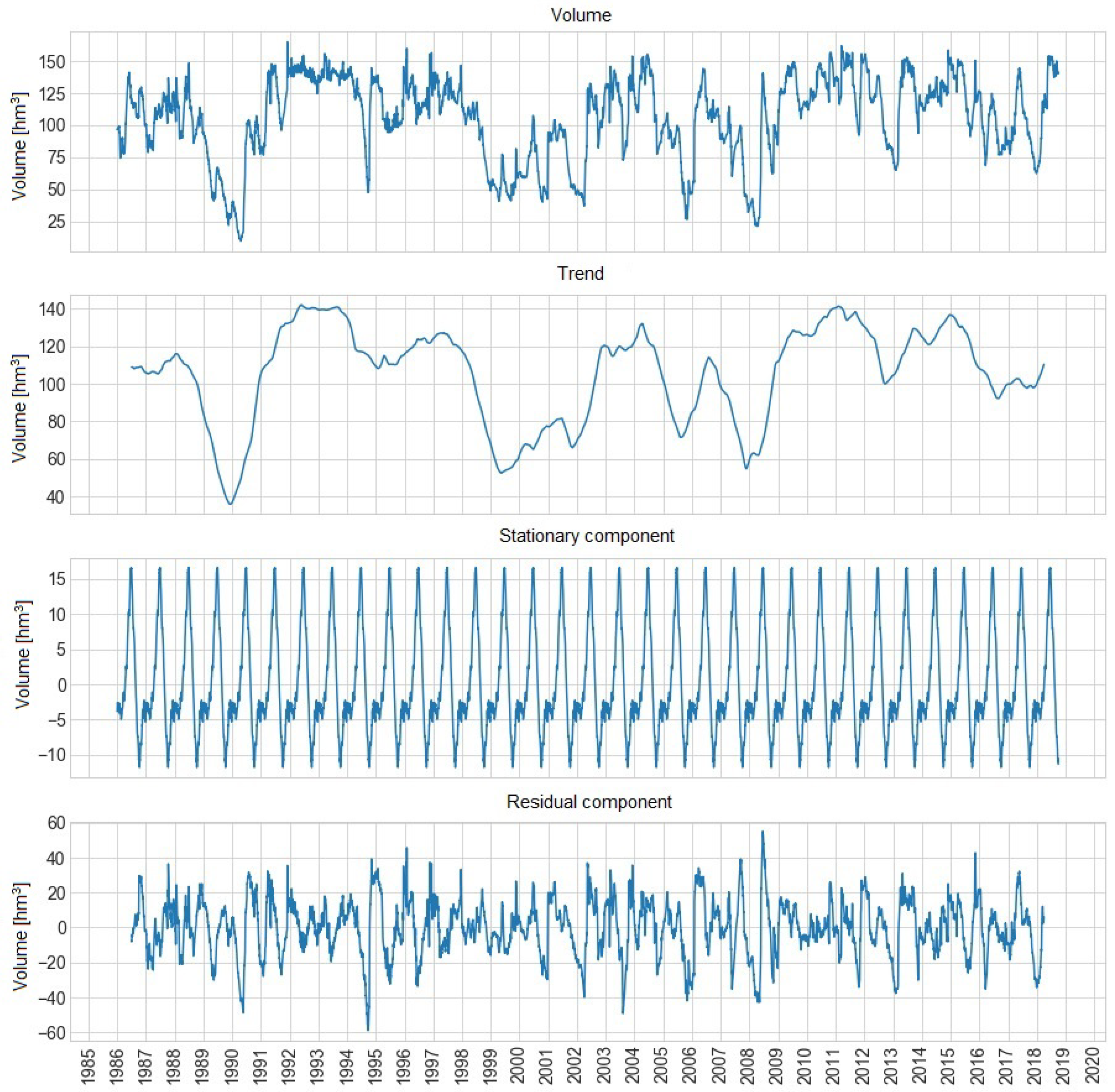
This section presents the statistical analysis of the main attribute, the volume data, from both Sau and La Baells reservoir. A statistical analysis in temporary series data allows to assure its suitability for forecasting techniques. The main characteristic of a temporary series is its dependency on the time. The dependence of time and past values is what differentiates the temporal series from the common statistical approaches, a dependency that prevents the assumption of independence from the explanatory variables based on the traditional methodology of attributive statistics. Temporary series are usually composed of three components: trend (T), seasonality (E) and residues or random variation (A). In this way each observation can be characterized as the sum of its components:

$$x_t=T_t+E_t+A_t.$$

(1)

Figure 1 shows the temporal decomposition of the volume of water from the Sau reservoir. This figure is composed of four different plots: volume of water, trend and, stationary and residual component in hm${}^3$ from 1996 to 2018.

We can observe how there is not a clear trend, the volume of the Sau reservoir does not tend to increase or decrease. However, this trend indicates the years of drought, showing a normal behaviour of temporary series depending on the seasons of the year. The seasonal component remains clear, with a seasonality in periods of year marking the maximum and minimum peak.

Further data study includes the Dickey–Fuller test [21]. Thus, we apply the Dickey–Fuller test to see if we have a stationary series already in origin. The seasonality of a temporary series is an important characteristic that can help us to produce satisfactory models, according to the revised literature. The mentioned test is a contrast of hypotheses where the null hypothesis of the test is that the series is not stationary; obtaining a p-value smaller than the level of significance, we can conclude that the series is stationary, when the null hypothesis is refuted.

Table 3. Dickey–Fuller’s test results of volume of water attribute from Sau reservoir.

Attribute	Value
Test statistic	−5.612817
p-value	0.000001
#Lags used	37
Number of observations used	11,923
Critical value (1%)	−3.430899
Critical value (5%)	−2.861782
Critical value (10%)	−2.566899

presents the results after applying the Dickey-Fuller test to the volume of water from the Sau reservoir.

Therefore, looking at the p-value, we can conclude that we have a stationary series already in origin, where the lack of trend is the key element of this stationary series, rather than its shape, which is certainly irregular. Thereby, we perform the predictions from the original series, because of its seasonality characteristics and, the data do not need transformations in this regard.

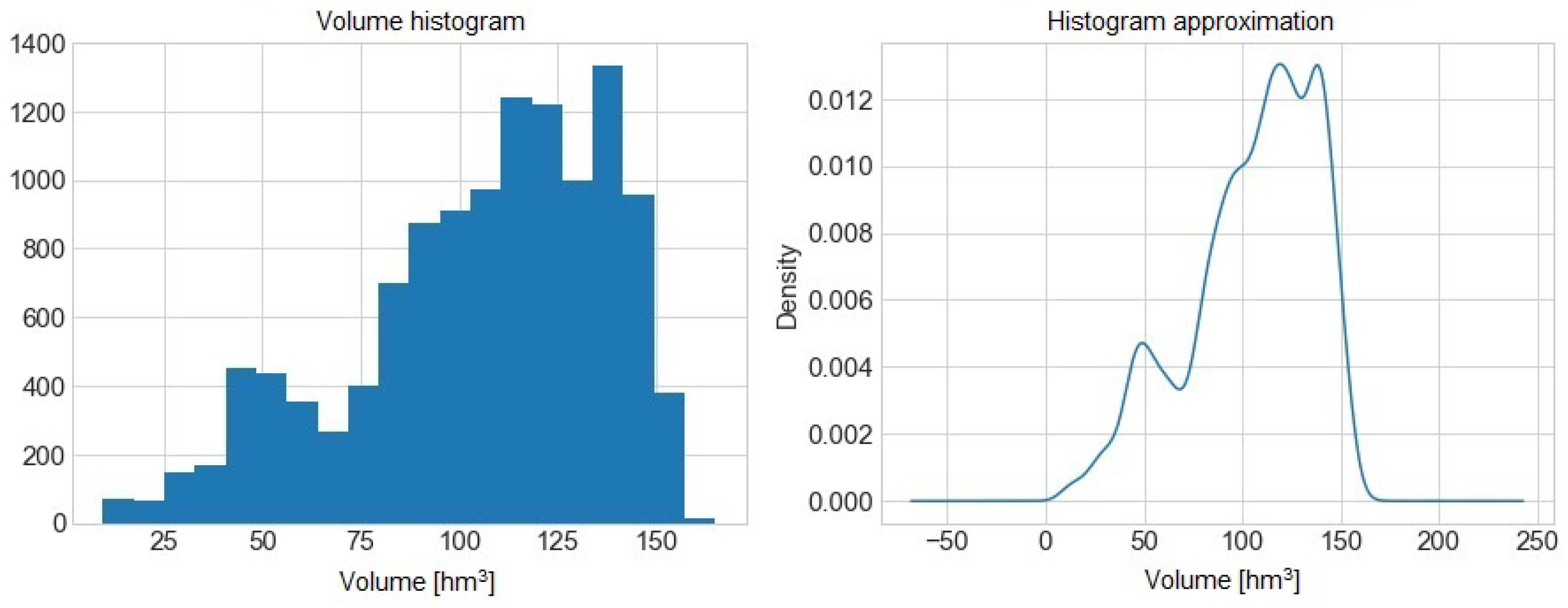
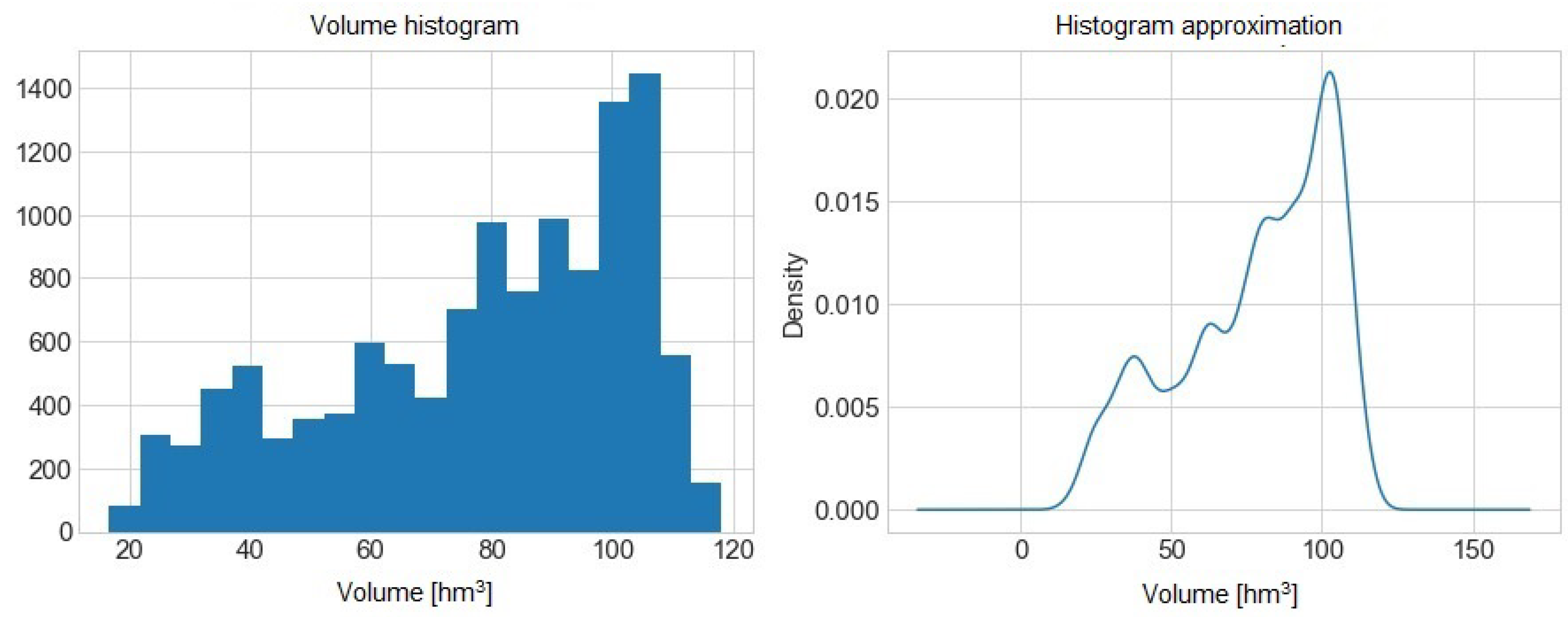
Figure 2 presents the histogram and its approximation of the volume of water from the Sau reservoir.

We can determine high balance values. We continue the study development as described in [3], to perform both the autocorrelation and the partial autocorrelation test, in order to determine the number of entries to be considered by the model.

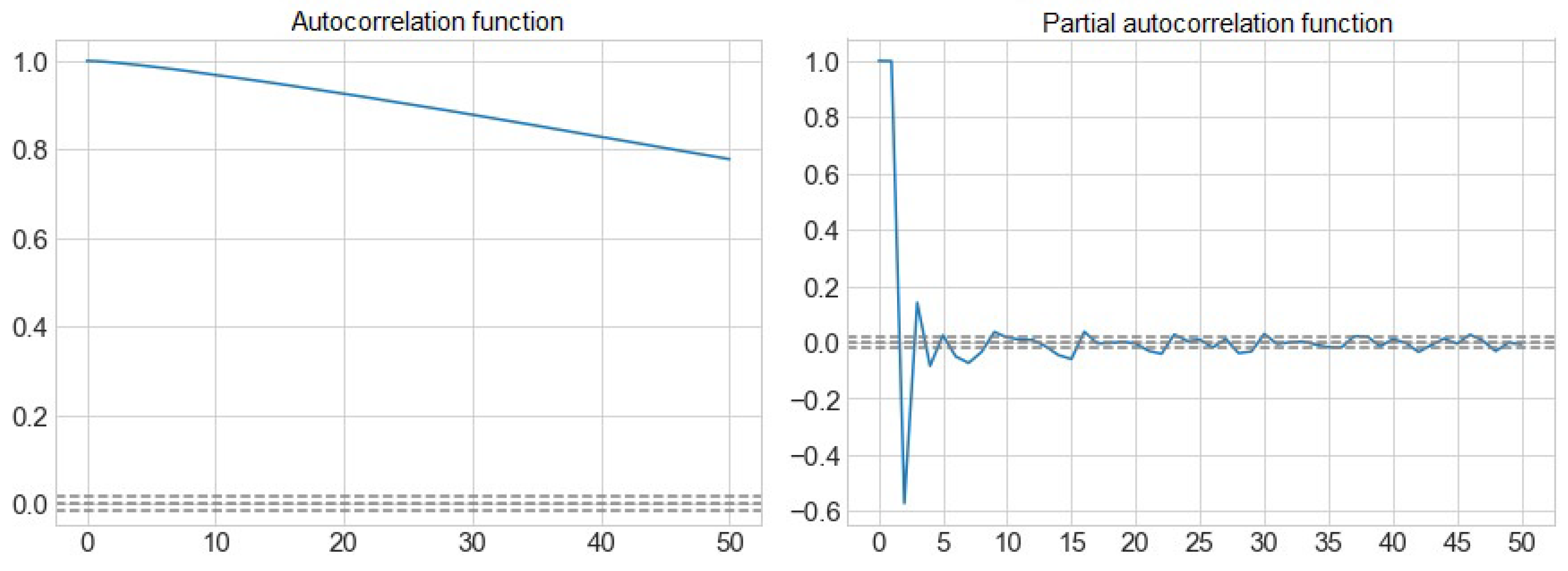
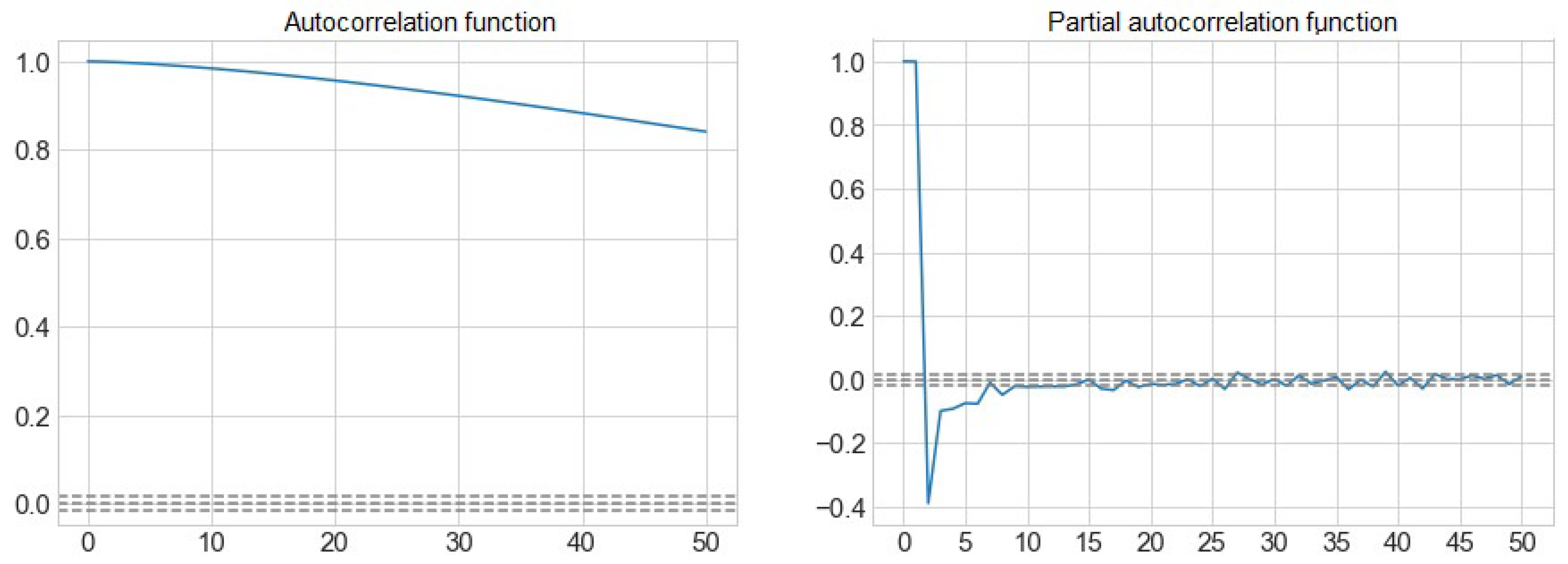
Figure 3 shows the autocorrelation function (ACF) and partial autocorrelation function (PACF) of the volume of water from the Sau reservoir.

We can observe how the sizes of the inputs to consider will be from t-1 to t-5, which is the first value that goes into the interval that determines the non-correlation, marked with a discontinuous line. At the t-17 we find the last correlated peak, from which the value is already within the confidence interval with a confidence level of 95%.

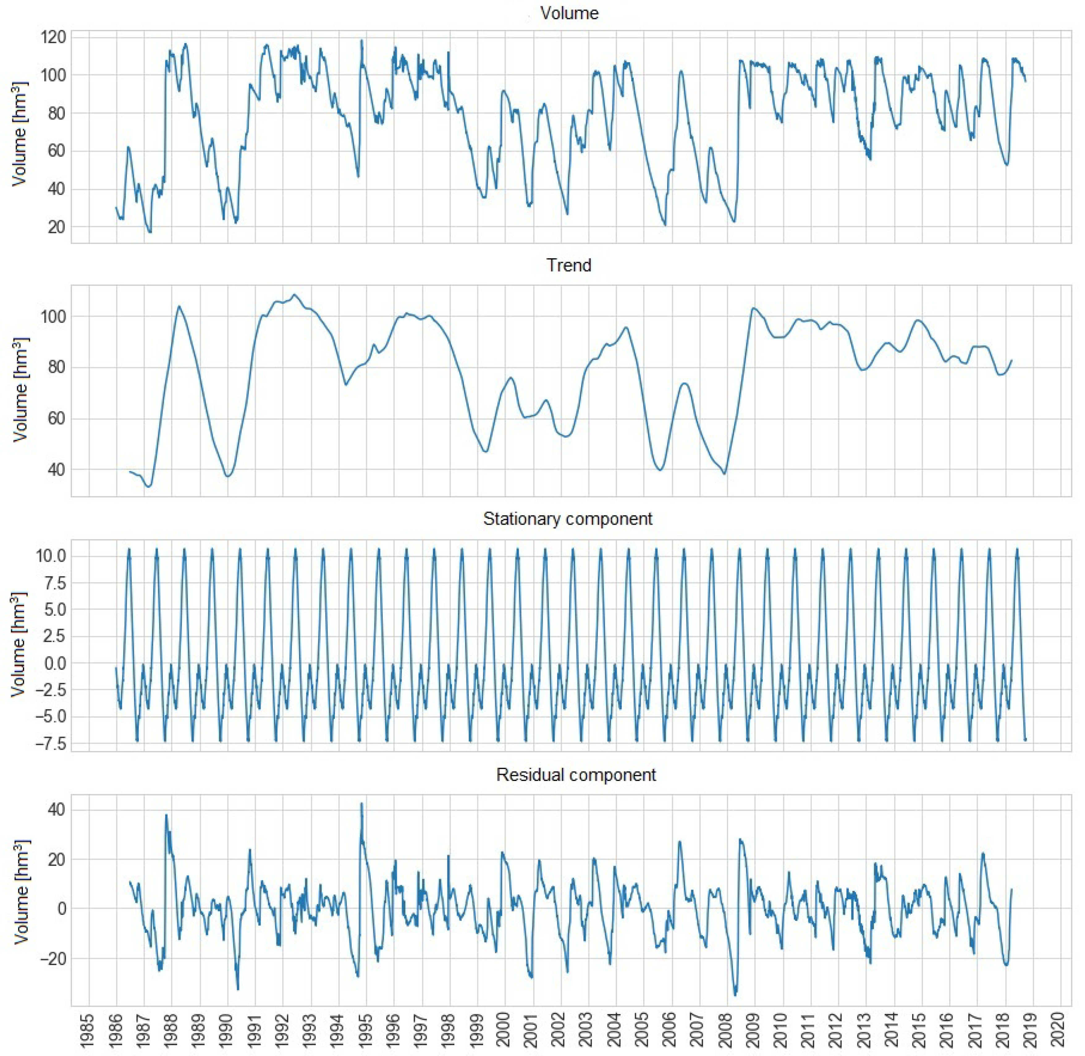
From the La Baells reservoir, we present the same results as shown above to assure the quality of the data for a posterior prediction implementation.

Figure 4 shows the temporal decomposition of the volume of water from the La Baells reservoir.

Along the same line of the Sau reservoir, there is no trend in the volume of the La Baells reservoir. Therefore, the chart follows a logical trend already described of years considering drought periods.

Table 4. Dickey–Fuller’s test results of volume of water attribute from La Baells reservoir.

Attribute	Value
Test statistic	−5.526781
p-value	0.000002
#Lags used	40
Number of observations used	11,920
Critical value (1%)	−3.430899
Critical value (5%)	−2.861783
Critical value (10%)	−2.566899

presents the results after applying the Dickey-Fuller test to the volume of water from the La Baells reservoir.

As in the previous case, looking at the p-value, we can conclude that the time series are clearly stationary.

Figure 5 presents the histogram and its approximation of the volume of water from the La Baells reservoir.

We have some balanced data for high volume reservoirs. Figure 6 shows the autocorrelation function (ACF) and partial autocorrelation function (PACF) of the volume of water from the La Baells reservoir.

In this case, after entry t-9, we are still within the confidence interval that allows us to conclude the non-correlation between the entries. Therefore, it is an information to take into account when it comes to modeling the number of entries for our model.

Once we analyzed the main attribute data for its prediction suitability, we introduced forecasting techniques used within the reservoir water level prediction.

4. Exploration of Forecasting Techniques

In this section, we analyze the predictive models proposed at Section 2, in order to highlight those aspects that are relevant and useful for our work. Therefore, we pay special attention to the methods and techniques used by the research that precedes us in this area of the prediction of water volume in hydroelectrical reservois. We start this analysis with one common approach for model prediction, i.e., neural networks. The first neuronal network to analyze is the one proposed by Rani and Parekh [22], made for predicting the volume of water in the Sukhi reservoir in India. In their research, 23 years of data were used with the daily information of input flow, flow of output and level of water. They used 16 years of data to train and seven years to make the evaluation of the model. The final model predicts data on the water level in the reservoir of 10 days after the information from the previous 10 days, which will be the entry of the model. The results are compared according to three types of neuronal networks: Cascade, Elman and feedforward back propagation. The latter type had the best response, with a root mean square error (RMSE) of 0.82.

Nwobi–Okoye and Igboanugo [5], on the other hand, make the prediction on the Kainji Dam, Nigeria. They used data from the daily water level between 2001 and 2010. The neuronal network is a feedforward multilayer perception (MLP). The function of activation of the neurons of the hidden layer is the sigmoid function. They parametrize the number of training iterations (epochs) to 1000. They establish a set of training corresponding to 75% of the data; the remaining 25% will be used as a test set. The research tries to find the architecture of the network that gives a better result among the five analyzed, increasing the entries of one to five, incrementally, in the same way as the number of neurons of the hidden layer. The best-performing architecture is composed of four input neurons, four neurons in the hidden layer and an output neuron, architecture (4-4-1), with a relative error of 0.065. They indicate that the good performance of the neural network depends on the design of the architecture. They corroborate this aspect from other studies such as Maier and Dandy [23] and [24]. This research allows us to propose architectures with specific neuronal networks, with their number of neurons per layer, activation functions and learning iterations. Furthermore, this study motivates us to explore not only one variable model, water level, but also the inclusion of more variables to model in a more complete explanatory and predictive level.

In the article by Üneş et al. [3], on the reservoir William “Bill” Dannelly, which is the name of the reservoir created by the Millers Ferry Dam in Alabama, United States of America, we find a comparison between models to try to predict the level of water in the reservoir. In this case, we obtained a better result of the model based on neural networks rather than models based on the analysis of temporal series using AR and autoregressive–moving-average (ARMA) models as well as multiple linear regression. Different behaviours are studied based on the entries, testing different combinations of entries for all models by trial and error. The best result model is the neuronal network with five input neurons, which obtains the following indicators: MSE = 0.0032; mean absolute error (MAE) = 0.0415 and R = 0.893, where MSE corresponds to mean square error; MAE, mean absolute error and R to the correlation coefficient. In this case, they used six years of historical data daily from the water level in the reservoir, which they distribute in 1461 days for the training and 811 for the test. The specific interest that this article has for our work is that it introduces some interesting indications to keep in mind the neural network architecture. For example, it is based on works such as Kisi et al. [13], Cybenco [25] and Hornik et al. [26], to justify that we can model any complex nonlinear relationship with a single hidden layer in the neuronal network. The number of neurons in this hidden layer is established by trial and error in an iterative manner.

Another important element that appears in the article is the use of methods of regularization, in this case through the Bayesian regularization, which allows us to finish adjusting the training of the model without undergoing training. We find a complete theoretical analysis on the techniques of regularization in [27]. We would also emphasize, in the face of our study, how to determine the input data vector, performing an autocorrelation and partial autocorrelation analysis, with the objective of constructing data vectors, optimal input. They set the length of the optimized input vector at five, corresponding to the five neurons of the input layer.

As we have seen, we have research based on the whole predictive model in a single variable, the daily volume of water in the reservoir. We take into consideration the fact that the level of the reservoir is the result of a complex set of environmental factors [3]. Thus, we prepare a list of factors that may intervene or depend on the level of water: precipitation, temperature, water temperature, water vaporization, etc. However, the researchers, based on the work in Şen et al. [28], quickly rule out the option of developing a more sophisticated model, which would include the mentioned explanatory factors, alleging economic and practical reasons. Hence, we introduce more variables to obtain more explanatory and predictive models.

Onidmu and Murase [19] discuss this same issue in their research on the prediction of the water level in Naivasha Lake in Nigeria. For these authors, the greater the number of groups of variables and the number of elements in each group of variables, the more predictive power of the neuronal network. They use data from 1960 to 1997, including water level per month, rain per month, evaporation of water, flood flow of the Malewa and Gilgil rivers and harmonics in time of the months of the year. They compute six models between which only the number of input neurons varies. The best model is the one with the smallest number of neurons in this layer, with an architecture (8-10-4). The model predicts four months from data from the previous six months. They train the neuronal network with the output weight optimization-hidden weight optimization (OWO-HWO) function. This best model gets a MSE of 0.12%. This model is interesting since it is the first, to the best of our knowledge, using more variables than just the water level [22].

Mokhtar et al. [8] propose a neural network model with architecture (5-25-1) to try to model the time period between rainfall and the rain is reflected in the volume of water in the reservoir of Timah Tasoh in Malaysia. It uses data from the daily water level in the reservoir from 1999 to 2006. Therefore, it is again another example of research that uses a single variable. The data is normalized before being entered into the neuronal network. Kilinç and Cigizoglu [29] predict the level of the Sungurlu reservoir, in western Turkey, through neural networks. In this case, the research focuses on the comparison of network training functions: radial base function (RBF) and feedforward back propagation (FFBP). They also cite the article by Coulibaly et al. [30], in which an exhaustive search of the articles related to the neuronal networks and the hydrology is realized. This article concludes that 90% of the cases use a direct neuronal network, feedforward neural networks (FNN), trained with back propagation (BP). The method of gradient descent is also often used in cases of hydraulic reserves, according to the authors themselves.

As mentioned above, Kilinç and Cigizoglu [29] compare a FFBP neuronal network with the behaviour of a neuronal network trained with the RBF. The results obtained in the comparison of models are not relevant, since they do not obtain significant differences, which is why they conclude that both networks are valid. In their work they include three variables: water flow, evaporation and volume of water. However, they do not generate a model that integrates them when it comes to predicting the objective variable, the volume of water. Nevertheless, they produce three models, one for each factor, where only one factor is taken into account in each case. It would have been interesting to see the integration of the three variables in a single model to predict the only real objective variable, such as the level of water in the reservoir. Dogan et al. [31] compile a comparison of neural networks similar to the research seen until now, on the Lake Van in eastern Turkey. The work done by Sen et al. [28] take into account the data of volume of water in the reservoir when developing the predictive model, despite recognising that this volume depends on different factors such as complex meteorological and geological. Therefore, we find that there may be some debate within the discipline to face these predictions with only one variable or multiple factors.

We emphasize this research by Dogan et al. [31], especially through the procedure, which has proved to be especially interesting and unmarked with the rest we have seen. It captures data from October 1975 to December 2011. These data are divided into groups of 10 years, which at the same time end up dividing into groups of three years for the training and two for the test. This way of proceeding allows to model a dynamic lake, that means, characteristics change over time. With this system, they intend to capture the pattern of these changes, which would allow them to make long-term predictions. To the best of our knowledge, it is the only article that proceeds in this way; the rest of papers have considered the chronological data as raw data training and left a part of the last to do the test; for instance, using the data from 2000 to 2009 for training and the year 2010 for testing. Another feature of this article is the mapping of water level data according to calendar dates. To carry it out, they compare two models of neural networks considering different entries: the first model uses the structure day-month-year, according to the Gregorian calendar; the second model uses the model based on the hydrological calendar, whereby October 1st is the first day of the year. In the second case entries are not separated by months: the entries will be the day number in relation to the hydrological calendar and the year. The second model achieves better results than the first one. In the case of the feedforward neural network (FNN) model, the architecture implemented includes a single hidden layer. The entries include the information of the date and the output is the daily water level. The function of activation of the neurons of the hidden and exit layer is the sigmoid function. The training is carried out with the Levenberg–Marquardt algorithm.

The results obtained indicate that FFNN models are imposed in all cases on the RBF neural networks, that is, the worst result with FFNN improves the best result of RBF. The best neuronal network has 90 neurons in the hidden layer and trains with 35 epochs, which are the two parameters to be configured for trial and error. This best model obtains a mean square error equal to 0.0012. The authors emphasize that the main difference of their model with regard to the literature is the prediction of future water levels based on all the observed data. This, according to them, is possible thanks to the data referenced to dates, both for the Gregorian calendar and the hydrological calendar. This indicates the mapping of the data according to calendar dates as the main and relevant novelty of this study, which allows to capture the trends of change in future predictions. In the same way Lake Van, in Turkey, together with Lake Egirdir, Çimen and Kisi [32] perform a comparison between neural networks and SVMs. Here, the level of the reservoir, also based on the work by Sen et al. [28], is used uniquely as a variable.

The training of the neural network is carried out through the function of Levenberg–Marquardt, whose authors consider a technique more powerful and faster than the “conventional” gradient descent technique. The best neuronal network is obtained with an architecture (4,8,1), with the hidden layer using neurons with sigmoid activation function and linear activation function for the output layer. The epochs were parametrized at 50. We explore the correlation analysis to determine the optimal input vectors for the system. In this case, beyond four consecutive data from the time series, there are no significant correlations, so the study focuses on entry vectors of $L_{t-1}$, $L_{t-2}$, $L_{t-3}$, $L_{t-4}$, analysing four type of inputs in the model. For the SVM model in Lake Van, the following parameters are used: Cc = 75, $ϵ$ = 0.003 and $\sigma$ = 0.0004 obtaining the best results with two $L_{t-1}$, $L_{t-2}$ entries, with a MSE of 0.0080. Lake Egidir gets better results with parameters Cc = 70, $ϵ$ = 0.008 and $\sigma$ = 0.23, in this case with four $L_{t-1}$, $L_{t-2}$, $L_{t-3}$, $L_{t-4}$ entries reaching an MSE of 0.0043. The significance of the differences in the comparison of the results obtained between models is carried out through analysis of variance (ANOVA) analysis. From this analysis, they conclude that the prediction differences between SVM and artificial neural networks (ANN) models are significant, with a confidence level of 95%. Thus, this article concludes a better result of SVM over neural networks, in all cases. It introduces procedural methods that we take into account, at the same time that they achieve remarkable results in both tested models. empirical evidence of the best behaviour of SVM is added, since in both cases they are superior. Empirical evidence that is not entirely conclusive, since in direct comparison with the work of Dogan et al. [31] and Lake Van, we see that the model based on neural networks of this latter is superior, since it obtains a lower MSE, in this case of 0.0012. The set of training data includes only 560 observations, for the 8036 observations used by Dogan et al. [31]. In this regard, we conclude that the best way to proceed is from daily data on water levels in the reservoir. We also highlight the research article by Hipni et al. [17], in which they develop a model based on SVMs, in order to overcome the prediction capacity of an ANFIS model, specifically, they aim to overcome the model proposed by Valizadeh and El–Shafie et al. [11], carried out at the same Malaysian reservoir, called Klang.

In Ali et al. [33], different models are proposed according to the specific objective they want to predict or classify. In the case of water levels in reservoirs, they compare the ARIMA model, two neuronal networks and the SVM model. The latter model obtains the best result with an RSME of 0.04, much higher than the 1.79 obtained by the second classifier model. They use SMOreg, whose authors define as an improved version of SVM, adapted for regression tasks. In this work, more than one variable is taken into account such as reservoir level, capacity, input flow, normal output flow, exceptional exits and losses. The data go from 2001 to 2012 without considering meteorological factors. We propose two articles related to decision trees as models for predicting water level in reservoirs. Jun–He Yang et al. [4] perform three simultaneous comparisons: the first corresponds to how to impute lost values; the second one performs an analysis of key factors, sequentially eliminating the least important; and the third is a comparison of prediction methods according to the data combinations of the two previous parameters: the attribution of lost values and the determination of key factors.

The models this articles compares are the following: the neuronal network with radial base function (RBF) and the classifiers Kstar, Random forest, k-nearest-neighbor (KNN) and random tree. They emphasize the importance of including a variable selection analysis because eliminating the least relevant models from the model has shown that it can improve the efficiency of model prediction, based on studies by Öztürk et al. [34], Vathsala and Koolagudi [35], Banerjee et al. [36] and, Yahyaoui and Al–Mutairi [37]. They also improve the accuracy of the model by selecting relevant variables based on the work of Borges and Nievola [38]. The selection of variables is carried out using the technique of factor analysis (FA). The order of importance of the variables that they obtain is the following: input flow, temperature, flow of output, pressure, precipitation, precipitation in Dasi, relative humidity, wind speed and wind direction.

They proceed iteratively, eliminating the least important variable until obtaining a minimum RMSE. The best result is obtained by eliminating the two less explanatory variables: direction and wind speed. Eventually, the final model is random forest, with the selection of variables, eliminating the two least relevant ones. Thus, this article introduces the decision trees as models to consider, namely a combination of these, the random forest, and a more detailed treatment of the variables that we include beyond the volume of water. The article by Pattama Charoenporn [39] makes a prediction of entry flow into the Huai Price Reservoir in Thailand through decision trees ID3 and C4.5. They take into account the flow of entrance and rain. Through the correlation between input and output, they determine the delay between the rain and the flow of input, in order to determine an entry of the appropriate model. The best model in this research is achieved with the ID3 algorithm, with an RSME of 0.1225. The researchers themselves indicate that neuronal networks can be a better alternative, as well as the use of more data and variables, as they have only taken into account three year rainfall data and input flow. Therefore, it is an article that reaffirms us in the line of research that we have considered for the present work.

Once analyzed and compared different state-of-the-art techniques, we will present the prediction methodology carried out.

5. Methodology and Results

This section describes the strategies and methods implemented on the selected reservoirs and, the results from the optimized simulations.

Since the goal of this research is the prediction of several days ahead, we follow a multi-step forecast where three different strategies can be distinguished [40]:

• Iterative strategy: A model which predicts the next one-step forecast and incorporates the predicted value to the model’s entry to predict the following. In this way, the following time steps are predicted, iteratively, one by one, updating the model with the values of the predictions.
• Direct strategy: It generates a model for each desired output. There will be a model predicting the next value of the time series $y_{t+1}$, another one that predicts $y_{t+2}$; but always based on real historical observations.
• MIMO strategy (multi-input multi-output): A single model that generates multiple outputs from multiple entries.

As a summary from Section 4, we explored the following state-of-the-art forecasting methods [27]:

• Neural Networks

  -

  Multilayer perceptron (MLP)

  -

  Convolutional neural network (CNN)

  -

  Long short term memory (LSTM)

• Support vector machine (SVM)
• Random forest (RF)

Combining the above list of strategies and techniques, we explored a large number of models. A model will be expressed with the technique acronym and the approach. For instance, using the support vector machine with the uni-variant approach would be named SVM-Uni. Due to space limitation, we will show uniquely the best six methods from each reservoir. Details about the chosen models and data specifications are displayed in

Table 5. Models and data specifications.

Reservoir	Model	Train	Test	n_steps_in	n_steps_out	Strategy
Sau	SVM-Multi	3412	854	11	15	MIMO
	MLP-Multi	3416	854	7
	SVM-Uni	2823	706	17
	LSTM-Uni	2812	704	30
	RF-Uni	5463	1366	5
	RF-Multi	3417	855	5
La Baells	SVM-Multi	3413	854	10
	MLP-Multi	3412	854	11
	SVM-Uni	2817	705	24
	MLP-Uni	2812	704	30
	RF-Uni	5463	1366	5
	RF-Multi	3412	854	11

. This table presents the number of samples used for training and test, the number of steps in and out and the strategy.

Note that the implemented techniques have been optimized where parameter values are:

• LSTM

  -

  Neuron LSTM layer: 5

  -

  Epochs: 1000

  -

  Learning rate: 0.0045

  -

  Batch size: 128

  -

  Optimizer: Adam

  -

  Activation function: sigmoid

  -

  Input days: 30

• MLP La Baells-Multi/La Baells-Uni/Sau-Multi

  -

  Neuron Hidden layer: 5/30/48

  -

  Epochs: 773/600/337

  -

  Learning rate: 0.001267/0.0006/0.00079

  -

  Batch size: 47/16/126

  -

  Optimizer: Adam/Adam/Adam

  -

  Activation function: sigmoid/sigmoid/sigmoid

  -

  Input days: 11/30/7

• SVM La Baells-Multi/La Baells-Uni/Sau-Multi/Sau-Uni

  -

  C: 85/124/25/24

  -

  Epsilon: 0.0115/0.0144/0.015/0.0127

  -

  Gamma: 0.0101/0.0852/0.010/0.2788

  -

  Input days: 10/24/11/17

• RF La Baells-Uni/La Baells-Multi/Sau-Uni/Sau-Multi/

  -

  Number of estimators: 120/303/362/140

  -

  Maximum number of features: 5/84/5/5

  -

  Maximum tree depth: 15/11/83/91

  -

  Minimum number of samples to split: 26/29/21/11

  -

  Minimum number of samples per leaf: 14/3/44/18

  -

  Input days: 5/11/5/5

The models will be evaluated using the root-mean-square error (RMSE), a measurement of own evaluation of the regression models, which is defined by the following formula:

$$RMSE=\sqrt{\frac{1}{\left|D\right|}\sum _{d\in D}{(f\left(d\right)-h\left(d\right))}^2},$$

(2)

where D is the set of observations, $h:X\to \mathbb{R}$ is the function of the model and $f:X\to \mathbb{R}$ is the objective function with the correct labels of the instances [27]. The main characteristic of this measure is that it expresses the error in the units of the data. Therefore, it allows us to evaluate the model in a contextualized way to the problem that it attempts to respond.

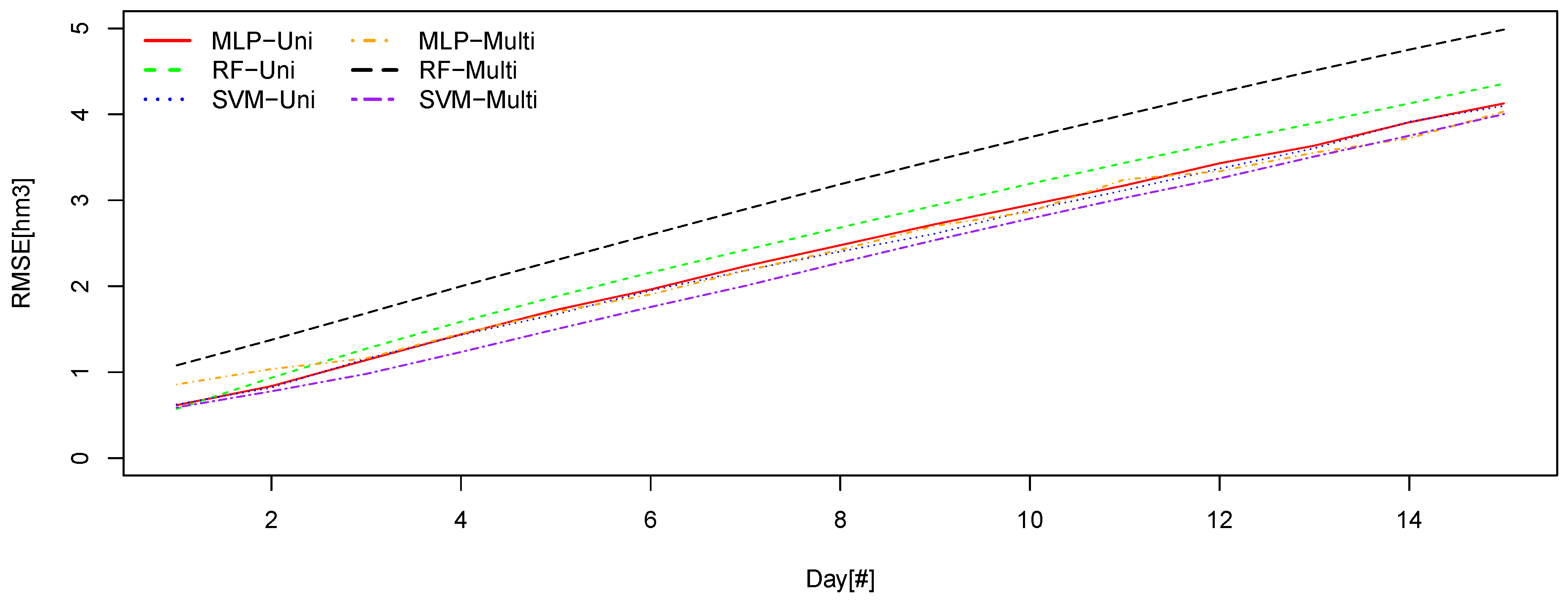
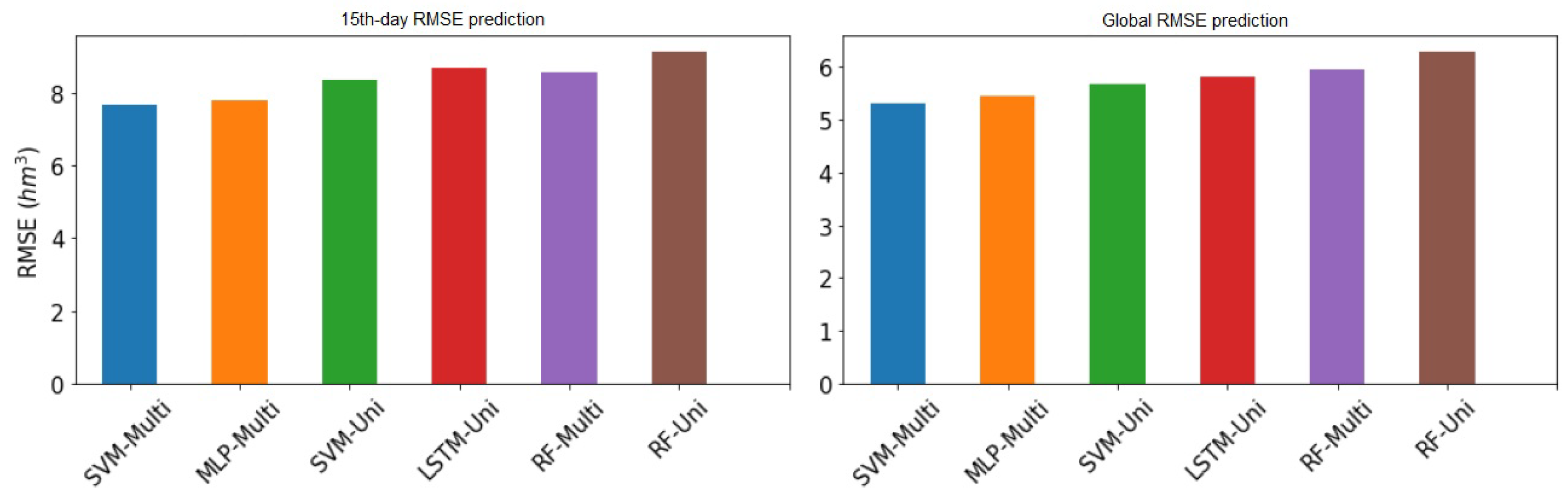
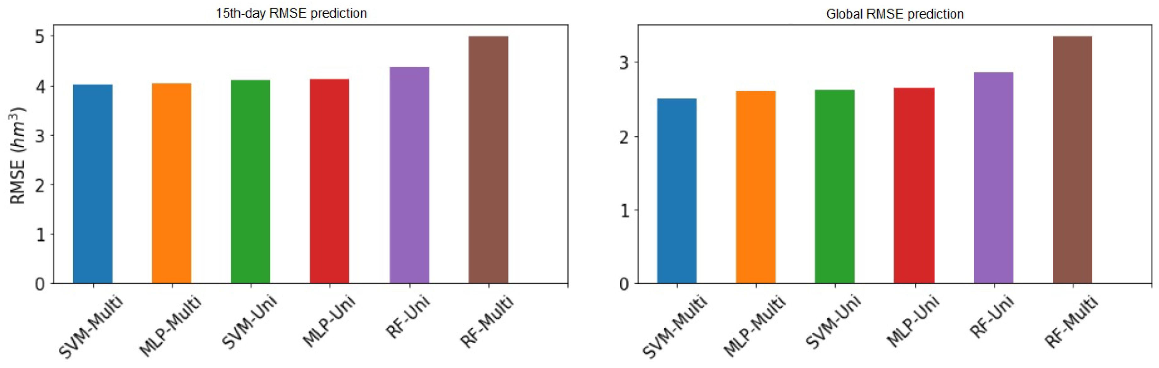
Figure 7 and Figure 8 compare the six best method and approach combinations with the lowest RMSE values along the time for Sau and La Baells reservoirs, respectively. Figure 9 and Figure 10 show the RMSE values at the 15th day and globally of all models presented above from both Sau and La Baells reservoir, respectively.

Using the multi-variant SVM model, the RMSE in overall provides the lowest values along the time.

If we compare the global error, graphically, we can see that the differences are very tight indeed. On the fifteenth day of prediction, the same thing happens to us, with a virtually total equality between the two best models. We can also see how the uni-variant LSTM model has more error on the fifteenth day than the Random forest multivariate, so there would be a change in classification taking into account only the fifteenth day.

Next, we will add some more metrics to evaluate the different models. We will do it through the mean absolute error and the coefficient of determination, also known as R-squared ($R^2$). The MAE is defined as:

$$MAE=\frac{1}{\left|D\right|}\sum _{d\in D}|f\left(d\right)-h\left(d\right)|$$

(3)

where, D is the set of instances, $h:X\to \mathbb{R}$ is the function of the model and $f:X\to \mathbb{R}$ is the objective function with the values of the real observations [27]. Following in [27], as well as the RMSE penalizes the greatest errors, in the case of the MAE all the waste has the same contribution in the calculation of the error. The penalty of the biggest errors comes from the square elevation of the difference between predicted and actual value, as we can see with the formula of RMSE that we have presented previously. The coefficient of determination puts in relation the variance explained by the model with respect to the real variance of the data [41]. It is a measure of the kindness of the model for the proportion between the variance explained by the variable’s model to predict the real variance of the variable. If this ratio is equal to 1, it will indicate that the model fully explains the variable to predict, therefore, the prediction would be perfect. The formula can be expressed in multiple ways, but we prefer the following that appears in [41] because it reflects the idea of the metric:

$$R=1-\frac{S{S}_{res}}{S{S}_{tot}},$$

(4)

where $S{S}_{res}$ stands for the sum of squares of residuals and $S{S}_{tot}$ refers to the total sum of squares (proportional to the variance of the data).

Table 6. The multi-variant SVM model returns the lowest RMSE and mean absolute error (MAE) values on Sau reservoir.

Model	15th Day			Global
	RMSE	MAE	${\mathit{R}}^2$	RMSE	MAE	${\mathit{R}}^2$
SVM-Multi	7.6907	5.7391	0.9130	5.2961	3.6088	0.9581
MLP-Multi	7.7908	5.9308	0.9107	5.4435	3.8811	0.9558
SVM-Uni	8.3699	6.3386	0.9065	5.6627	3.7640	0.9568
LSTM-Uni	8.6653	6.7872	0.8998	5.8064	3.9718	0.9546
RF-Multi	8.5605	6.7438	0.8921	5.9549	4.3192	0.9470
RF-Uni	9.1335	6.9229	0.8716	6.2832	4.2043	0.9662

shows the RMSE, MAE and $R^2$ results on the 15th day and global on Sau reservoir. The best results are achieved with the multi-variant SVM model. Furthermore, the MAE error, which is expressed in the same units as the data and that RMSE, is lower in all cases; therefore, the most important errors are penalising the error of RMSE. We also note that, looking at the MAE, the classification varies: the uni-variant SVM would pass in front of multi-variant MLP and the uni-variant RF would be ahead of the multi-variant, to the global extent. This means that these models provoke fewer errors, but they make them bigger, which is why they penalize the RMSE. On the other hand, we can verify that we obtain a very acceptable $R^2$ determination coefficient, even in the worst model and day, which would be the 0.87 uni-variant RF on the fifteenth day.

The first thing to emphasize is the range of values, very different from that of Sau, as we have already said. In this case, we return to have very tight results for the top part of the classification. In the global RMSE chart there is only 4% difference between the first and second models; between the second and fourth, 1.8% of RMSE. Certainly, the difference is wider between the first and last ones than in the case of the Sau swamp, with 25% more RMSE. We would also emphasize the equality between the models SVM and MLP, practically identical, except for the best model, which differentiates a little more. Regarding the graph of the errors to the fifteenth day, in this case, we did not find any alteration of the order with respect to the classification by global error. Give emphasis to the equality of the first four models.

Table 7. The multi-variant SVM model returns the lowest RMSE and MAE values on La Baells reservoir.

Model	15th Day			Global
	RMSE	MAE	${\mathit{R}}^2$	RMSE	MAE	${\mathit{R}}^2$
SVM-Multi	4.0029	2.4098	0.9515	2.5085	1.3506	0.9811
MLP-Multi	4.0330	2.7339	0.9508	2.6122	1.6148	0.9795
SVM-Uni	4.0985	2.6003	0.9537	2.6198	1.4503	0.9812
MLP-Uni	4.1279	2.8958	0.9531	2.6569	1.5905	0.9806
RF-Uni	4.3563	2.7258	0.9243	2.8514	1.4887	0.9677
RF-Multi	4.9869	3.5642	0.9248	3.3500	2.1372	0.9396

shows the RMSE, MAE and $R^2$ results on the 15th day and global on La Baells reservoir.

The worst model on the fifteenth day of La Baells has an $R^2$ higher than the best model of Sau, 0.9248 of multi-variant RF for the 0.9130 of the best model of Sau. We can also verify that global $R^2$ values are good enough. Analysing the MAE, we reaffirm multi-variant SVM as the best model.

If we consider the predictions of the Sau reservoir, then those in La Baells reservoir would be spectacular. Although the RMSE is not directly comparable, dimension difference between both reservoirs do not justify the error gap from the models. However, the data from the Sau reservoir have been much more difficult to model than those of La Baells. Therefore, with worse results, the result of the best model of Sau can be more valuable than one of the best model of La Baells.

Models studied in the literature predict the level of water in meters above sea level (MAMSL). This would explain their results with RMSE values close to zero.

Table 8. Our work outperforms related literature studies.

Work	Unit	Intervals	Timesteps	RMSE	${\mathit{R}}^2$	Others
Rani and Parekh [22]	MAMSL	135–148	10	0.82	0.95
Üneş et al. [3]	MAMSL	23.5–24.6	1	0.057	0.893
Onidmu and Murase [19]	MAMSL	1886–1888	4			0.12 (%MSE)
Kilinç and Cigizoglu [29]	Volume (hm${}^3$)	47–153	1	7.63	0.86
Dogan et al. [31]	MAMSL	1647–1650	1	0.035	0.93
Çimen and Kisi [32]	MAMSL	1647–1650	1	0.073	0.985

compares the main articles that we have analyzed with their predictions achieved.

In the timesteps column, we have the predicted future values of the corresponding time series of each proposed model. For instance, with a range of values ranging from 1647 to 1650 m, where predictions move at 3 m, the error will be smaller than predictions on wider ranges (i.e., 12 m). Therefore, this justifies these tiny RMSE values, which we cannot compare. Thus, when we predict the volume, as in the case of Kilinç and Cigizoglu [29], then we no longer have such ranges of values so short, as in the case of meters above sea level, and the error increases. In comparison with the literature, our research considers the prediction on volume and also through the determination coefficient, which evaluates the explanatory capacity of the model.

In terms of $R^2$, our models are similar to the literature. The worst model is the uni-variant RF on Sau reservoir with a global value of 0.94, which is better than three out of the five results from Table 8. Our best model, the multi-variant SVM of La Baells which returned an $R^2$ of 0.981, is better than all of them except for Çimen and Kisi [32] with 0.985. Nevertheless, if this last mentioned model makes a prediction at a time step, then we should compare it with the value of $R^2$ we get for the first day of our model, which is 0.99.

Comparing the results with the only research article predicting the volume of water [29], we achieved better results. They obtained an RMSE of 7.63 hm${}^3$ and, according to the range of volume of water from 47 to 153 hm${}^3$, we may compare it with the study of the Sau reservoir (9.5 and 165 hm${}^3$). In this case, the best and worst model returns an RMSE of 5.30 and 6.28 hm${}^3$, respectively. Therefore, our models outperform state-of-the-art works.

Note that models with the best overall result are those that have the best results on the fifteenth prediction day, specifically, and generally in the longest-term prediction. Since in the long-term prediction is where we accumulate more errors, an improvement in these days supposes an outstanding improvement in the global model. The models with the best overall result do not have to be those that refine the prediction to one day, as in the case of multi-variant MLPs, which we have already seen are beginning to be the worst to end up practically in line with the best, both in the last days of prediction and in the overall result.

6. Conclusions and Future Work

Reservoirs are natural or artificial lakes used not only to keep and manage large volume of water, but also to generate electricity when water exits the dam. In this paper, we presented a comparison of state-of-the-art forecasting techniques using real data from Catalan reservoirs. The data was composed of reservoir information such as volume of water and flow of entry, and meteorological data such as temperature, rainfall and wind speed. These data have been acquired from public online sites.

The data of heat and weather coincided with good quality in temporarily large enough bands to be able to handle them. It is plausible to think that input and output flow data had helped multivariate prediction, especially input, which reflects the effect on the rain or snow dam. Thus, we might think that the effect of rainfall, the flow of entry, may be more relevant than the rain itself. This would open us the most difficult debate of multivariate analysis, which is to know what attributes are necessary to treat, a question that is not easy, since we have seen that the accumulation of sediments can vary the capacity of a reservoir. We compared the most used methods: neural networks, SVM, and random forest. SVM returned the best results in both in the multi-variant and in the uni-variant analysis. Although results of the neural networks have been very close to the SMV, there is no point in comparing because of the computational cost. Results returned a longer prediction with higher precision than state-of-the-art related works. Thus, if we observe the R² value, we can find how our worst case model, uni-variant random forest (global R² of 0.94) outperforms some works from Table 8. Comparing the first step prediction, we achieve an R² value of 0.99, which is higher than the values presented in literature.

As future work, we plan but not limit to model a reservoir so that it has the possibility of being able to generalize (focus the modelling of a reservoir so that it can be used in each case), include different natural events such as snow and landslides or, study other sophisticated techniques such as deep learning.