Resources and Future Availability of Agricultural Biomass for Energy Use in Beijing

Abstract

The increasing importance of lignocellulosic biomass based energy production has led to an urgent need to conduct a reliable resource supply assessment. This study analyses and estimates the availability of agricultural residue biomass in Beijing, where biomass energy resources are relatively rich and is mainly distributed in the suburbs. The major types of crops considered across Beijing include food crops (e.g., maize, winter wheat, soybean, tubers and rice), cotton crops and oil-bearing crops (e.g., peanuts). The estimates of crop yields are based on historical data between 1996 and 2017 collected from the Beijing Municipal Bureau of Statistics. The theoretical and collectable amount of agricultural residues was calculated on the basis of the agricultural production for each crop, multiplied by specific parameters collected from the literature. The assessment of current and near future agricultural residues from crop harvesting and processing resources in Beijing was performed by employing three advanced modeling methods: the Time Series Analysis Autoregressive moving average (ARMA) model, Least Squares Linear Regression and Gray System Gray Model (GM) (1,1). The results show that the time series model prediction is suitable for short-term prediction evaluation; the least squares fitting result is more accurate but the factors affecting agricultural waste production need to be considered; the gray system prediction is suitable for trend prediction but the prediction accuracy is low.

1. Introduction

Biomass, as an important alternative energy source to conventional fossil fuels, has received major interest in recent years due to the progressive exhaustion of fossil fuels and the continually increasing demand for energy on a global level [1]. Biomass has a high potential to reduce greenhouse gas emissions while minimizing environmental pollution [2]. However, the amount of biomass supplies presents a large degree of uncertainty due to raw material cost fluctuations, variations in biomass seasonality and so forth. In order to evaluate the feasibility of introducing biomass-derived energy applications, it is necessary to conduct an assessment of the resources and their availability [3].

As one type of renewable energy, agricultural residue has been widely seen as an effective substitute for conventional fuels such as petroleum, gas and coal [4,5]. Collection of agricultural waste for bioenergy use and promotion is one of the most important state affairs [6,7]. Various methods have been proposed on the availability of different biomass resources in the literature. Gonzalez-Salazar et al. proposed a new method to determine key variables by using sensitivity analysis and probabilistic propagation of uncertainty and the method was applied to energy scenarios in Colombi. The proposed method significantly reduced the predicting uncertainty of both theoretical and technical biomass potential [8]. Maqhuzu et al. devised a quantification method that included the application of a probability distribution to strictly handle the uncertainty when quantifying the biomass and was simulated 100,000 times with the Monte Carlo method. The results showed a lower potential than previous estimates by employing the stochastic model instead of deterministic models [9]. Moreover, an integrated assessment method for understanding the availability and utilization potential of different biomass resources was presented by Hossenet et al. [10]. A novel feature of the developed method is the unconventional quantitative assessment of major biomass resources, which were previously ignored [10]. Welfle et al. determined the most promising indigenous biomass resources for the UK bioenergy industry and assessed the impact of different supply chain drivers on biomass availability with “A Biomass Resource Model,” which can simulate the whole system dynamics of biomass supply chains [11]. Vávrová et al. proposed an integrated method for empirical data (GIS) and detailed spatial data to assess both standard and additional biomass potential. The results showed that biomass potential from forest land and agriculture can be increased significantly in the short term [12]. According to the state of the technology, by defining explicit and rationale restrictions on sustainable bio-energy industry, Burg et al. estimated the potentially available woody and non-woody biomass resources for bioenergy in Switzerland using bottom-up approaches, which can be transferred to other study areas based on the local situation and available data [13]. Zhang et al. first used a quantitative universal exergy to evaluate the woody biomass potential and its impact on the environment [14]. Brahma et al. proposed a species-specific power-law model for rubber trees, which predicted biomass availability more precisely than universal models [15]. Chinnici et al. evaluated the potential available quantities of five types of agricultural waste in Sicily. The evaluation was based on statistics by applying parameters derived from the literature and direct research [1].

There are many proposed models and prediction models used for the assessment of potential biomass energy production in China as well. Ji conducted an assessment of agricultural residue resources and forecast the corresponding theoretical output in the near future using an artificial neural network (ANN) model for liquid biofuel production in China [16]. Zhao predicted the potential biomass production from 2030–2050 in China, based on the resource availability of five sources: agricultural crop residues, forest residues and industrial wood waste, energy crops and woody crops, animal manure and municipal solid waste [17]. Zhang et al. established the Long-range Energy Alternative Planning System (LEAP)-Beijing model for the medium-to-long-term greenhouse gas (GHG) emissions prediction in Beijing [18]. Hao et al. reviewed the current status, future potential and policy implications of biofuel for vehicle use in China [19]. Qin et al. performed a review of bioenergy resources from existing conventional crop (e.g., corn, wheat and rice) residues and energy crops (e.g., Miscanthus) and the impacts of biofuel production on ecosystem services based on the biofuel’s life cycle analysis [20]. Chen employed a mathematical programming model to estimate the economic potential of biomass supply from crop residues in China. The results showed that the crop residues supply relies on the yields and production costs of crop residues and biomass prices [21].

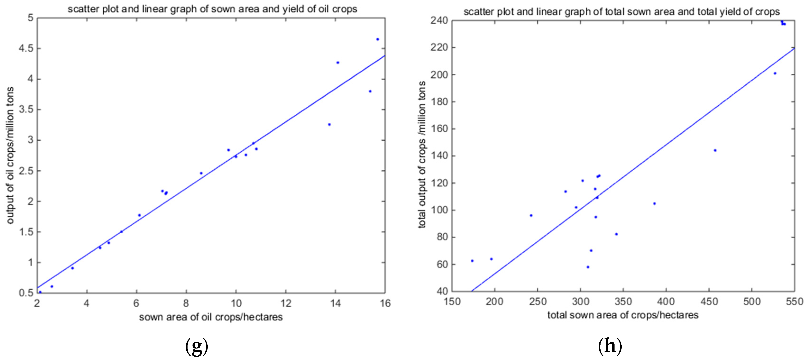
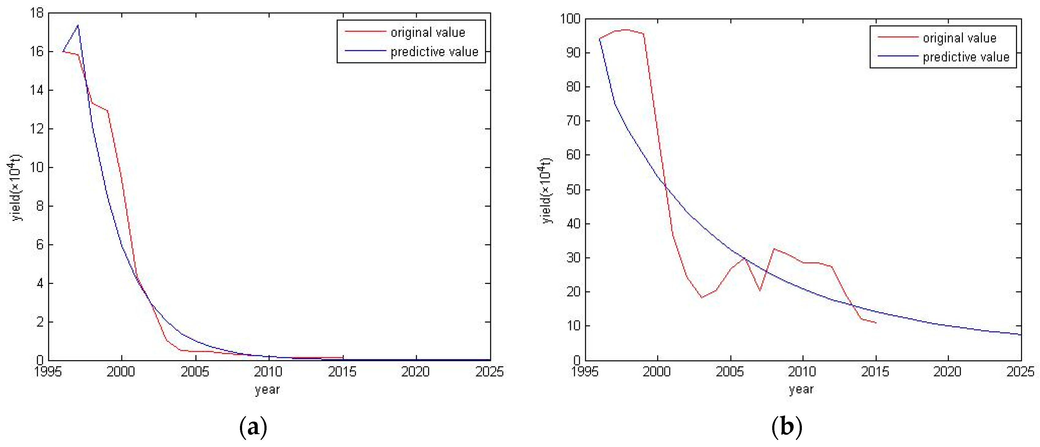
Agricultural residues play an important role in China’s biomass feedstocks because China is a vast agricultural country. However, direct combustion is still the main use of agricultural residues, especially in China’s rural areas. The ineffective use of agricultural residues leads to many problems. This study analyses the availability of agricultural biomass for energy use in Beijing, China, and in particular to be used for the production of biofuel. Advanced modeling methods, including the Time Series Analysis ARMA model, Least Squares Linear Regression and Gray System GM (1,1), are used for the prediction of biomass.

2. Methodology

2.1. The Resource Base

Among Beijing’s renewable energy resources, according to the preliminary surveys [2,22,23], the availability of biomass energy accounts for the highest proportion, which is 39.5%, followed by solar energy (31.9%) and geothermal energy (27%), respectively [23]. Beijing’s biomass energy resources are relatively rich, and are mainly distributed in the suburbs and the biomass energy type mainly includes agricultural waste, forestry waste, fecal residue, waste water and household garbage [24].

The estimate of biomass for the various categories of matrices used in Beijing was made by determining the potentially available quantity according to the type of biomass considered, which are agricultural residues from crop harvesting and processing for the present study.

In this study, the definition of agricultural residues is clarified as the total byproducts of field production (field residues hereafter) and the processing industry (process residues hereafter) [25]. Field residues are materials left in an agricultural field after the crop has been harvested and usually include straw, stalks, stubble, leaves seed pods and so forth. Process residues are materials left after the crop is processed into a usable resource and usually include husks, seeds, bagasse, molasses and roots and so forth. [23]. The major types of crops across Beijing include food crops (e.g., maize, winter wheat, soybean, tubers and rice), cotton crops and oil-bearing crops (e.g., peanuts). The theoretical maximum potential of crop residues can be estimated on the basis of the agricultural production for each crop, multiplied by specific parameters. The specific parameter refers to average Residue-to-Product-Ratios (RPR) for field residues or the process residue index (PRI) for process residues. Both are collected from the literature. The agricultural production for each crop can be sourced from Beijing Municipal Bureau of Statistics [26].

However, not all theoretical maximum potentials of crop residues were available. The residue availability varies significantly with climatic conditions and local agricultural practices [27,28]. These factors have to be taken into consideration when estimating the available supply of residue biomass. A collectable coefficient was defined for each crop, to incorporate the impact of all these factors. The quantity of the potentially available plant waste was a sum of the theoretical maximum potential of crop residues multiplying the collectable coefficient for each crop.

2.2. Advanced Modeling

This section will focus on the introduction of the Time Series Analysis ARMA model, Least Squares Linear Regression and the Gray System GM (1,1), which are used for the prediction of residue biomass in the future. They are all computational methods and useful empirical tools. Taking into account the special nature of crop straw yield influenced by historical data, the time series Analysis ARMA model can provide robust, stable and accurate prediction results in short- and medium-term forecasting. In addition, from the historical data, it is found that there is a strong positive correlation between sowing area and the yield of crop straws. Thus, the prediction using least squares linear regression can obtain more accurate results compared with actual values. The Gray system GM (1,1) is more suitable for long term forecasting with cases of incomplete data or without regularity to conform to. In this study, MATLAB 2014b is employed for the analysis.

2.2.1. Time Series Analysis ARMA

In the analysis of a time series containing relevant information, pre-processing of the data is necessary, followed by observing whether it can be identified as a stationary non-white noise sequence. If it is, an ARMA model is established to fit the sequence and extract useful information [29]. In this study, the classical time series model predicts the future trend of agricultural residue production from the historical laws of crop production. Due to changes in crop production over time and the special characteristics of current changes in quantity affected by that in previous periods, the autoregressive model is used to predict crop production in subsequent periods:

$$Y_t=a{Y}_{t-1}+b$$

(1)

where Y_t is the predicted value of straw yield at time t, Y_t−1 is the observed value of straw yield at time t − 1, a is the autocorrelation coefficient and b is the random disturbance.

2.2.2. Least Squares Linear Regression

Least squares linear regression is a computational method for studying the correlation between two variables. This method divides variables into independent and dependent variables. By establishing a linear relationship between independent and dependent variables, the intrinsic rules between the variables are revealed and the observed values of the dependent variables are predicted based on the given observed values of the independent variables [30]. In this study, the crop area (in thousands of hectares) is set as an independent variable and the crop yield (in ten thousand tons) is the dependent variable. The assumed model is expressed as:

$$Y=aX+b$$

(2)

where X is the area planted for a certain crop in a given period, Y is the predicted value of the straw yield of a certain crop in a certain period, a is the slope of the linear fit and b is the corresponding intercept.

2.2.3. Gray System GM (1,1)

If the information and features in a system are partially known and partially unknown, the system is a gray system. Most traditional statistical forecasting models require a certain number of historical data, which may not be completely available in many practical situations. The Gray system is suitable for cases of irregular or incomplete information [31]. In this study, the Gray system GM (1,1) is used to predict crop yield. The Gray system theory takes all random numbers as gray numbers, which will be analyzed using data processing methods to find the inherent rules between data. A new data sequence will be created through the processing of known data to study the regularity of the data. The essence of the Gray system theory is to accumulate irregular raw data for data sequence and then re-mode it. The gray differential equation model of GM (1,1) is:

x⁽⁰⁾(k) + az⁽¹⁾(k) = b

(3)

where x⁽⁰⁾(k) is the gray derivative, a is the development coefficient, z⁽¹⁾(k) is the whitening background value and b is the gray action amount.

From the above, we can see that different forecasting methods have different characteristics and it is difficult to clarify which method is the best. In practice, it is necessary to select a reasonable method based on data types and characteristics and the applicable conditions of different methods. Moreover, the combination of different prediction methods supplies a gap to a single method.

2.3. Data Collection

Crop residue yields varied for each crop depending on genotype and environmental factors [32]. Therefore, the Residue to Product Ratio (RPR) for field residues and Process Residue Index (PRI) for process residues were set as a range in literature, not a constant. For example, Guo et al. presented a series of range values of process residues factors for different crops [33].

Table 1. Residue to Product Ratio (RPR) and Process Residue Index (PRI) for major crops in Beijing.

Major Crops	RPR	PRI
Rice	2 [34,35]	0.18 [33]
Wheat	1 [34,35]	n/a
Maize	2 [34,35]	0.16 [33]
Tubers	1 [34,35]	n/a
Beans	1.5 [34,35]	n/a
Cotton	3 [36]	0.47 [33]
Peanuts	2 [36]	0.27 [33]

gives an overview of various averaged estimates for yields of crop residues as available from the literature.

Table 2. Agricultural yield (10⁴ t) of main crops from 1996–2017.

Year	Rice	Wheat	Maize	Tubers	Beans	Cotton	Peanuts
1996	16.00	93.90	119.70	2.60	2.30	0.25	2.88
1997	15.80	96.40	118.90	2.40	2.30	0.22	2.69
1998	13.30	96.70	122.60	2.30	2.50	0.18	2.78
1999	12.90	95.50	86.70	2.40	2.00	0.19	2.70
2000	9.36	66.86	58.70	3.02	4.71	0.16	3.36
2001	4.30	36.60	53.90	3.50	4.80	0.34	4.13
2002	2.90	24.30	46.10	3.70	3.50	0.35	4.58
2003	1.01	18.41	32.20	2.88	2.82	0.34	3.26
2004	0.50	20.26	43.51	2.21	2.98	0.78	2.86
2005	0.46	26.74	62.58	2.10	2.30	0.21	2.46
2006	0.43	30.01	72.91	2.58	2.49	0.22	2.14
2007	0.32	20.39	76.54	2.86	1.45	0.20	2.17
2008	0.30	32.74	87.97	1.88	1.91	0.14	2.13
2009	0.24	30.95	89.76	1.66	1.49	0.08	1.77
2010	0.19	28.38	84.17	1.36	1.07	0.05	1.50
2011	0.15	28.37	90.34	1.28	1.08	0.05	1.32
2012	0.13	27.44	83.58	1.22	0.89	0.03	1.24
2013	0.13	18.70	75.18	0.78	0.80	0.015	0.91
2014	0.13	12.20	50.04	0.68	0.60	0.011	0.61
2015	0.14	11.09	49.45	0.84	0.65	0.010	0.52
2016	0.12	8.54	43.19	0.87	0.44	0.006	0.44
2017	0.07	6.16	33.21	0.61	0.47	0.002	0.53

presents the yields of main agricultural products of different crops from 1996–2017 collected from the China Municipal Bureau of Statistics [37].

As seen from Table 2, it is found that the agricultural yields decrease dramatically from the years before 2000 to the years after it, especially for three cereal crops (rice, wheat and maize). The other crop types do not show obvious fluctuations and change smoothly. The trend of decreasing may be due to the policy of returning farmland to forest and grass, which started in practice since 2000 and almost finished in 2004. Therefore, three mean values (low, medium and high) of agricultural yields are calculated, as shown in

Table 3. Averaged agricultural yields (10⁴ t) of different crops.

Mean	Rice	Wheat	Maize	Tubers	Beans	Cotton	Peanuts
Low (2004–2017)	0.24	21.57	67.32	1.50	1.33	0.13	1.47
Medium (2000–2017)	1.16	24.90	62.96	1.89	1.91	0.165	2.00
High (1996–2017)	3.59	37.76	71.87	1.99	1.98	0.174	2.14

. The three mean values are corresponding to three time phase: 2004–2017 (after the policy is finished), 2000–2017 (the policy started in practice) and 1996–2017. The average yields were used as the baseline crop yields data for further analysis. Note that exceptions exist for maize, of which the medium value is the smallest. For cotton, the medium and high values are equal.

In the literature, a collectable and usable coefficient was used to estimate the collectable and utilizable amount of agriculture residues as a bioenergy resource [23]. In this study, the collectable coefficient of 23.9% [23] was used.

3. Results and Discussion

3.1. Current Availability of Agricultural Residues

The theoretical maximum potential (

Table 4. The theoretical maximum potential availability (10⁴ t) of crop residues.

Crop Types	Residue Types	Mean
		Low	Medium	High
Rice	Field residues	0.47	2.32	7.17
	Process residues	0.04	0.21	0.65
	Total	0.52	2.53	7.82
Wheat	Field residues	21.57	24.90	37.76
Maize	Field residues	134.63	125.93	143.75
	Process residues	10.77	10.07	11.50
	Total	145.40	136.00	155.25
Tubers	Field residues	1.50	1.89	1.99
Beans	Field residues	2.00	2.87	2.97
Cotton	Field residues	0.38	0.50	0.52
	Process residues	0.06	0.08	0.08
	Total	0.44	0.57	0.60
Peanuts	Field residues	2.94	3.99	4.27
	Process residues	0.40	0.54	0.58
	Total	3.34	4.53	4.85

) and collectable potential (

Table 5. The collectable potential availability (10⁴ t) of crop residues.

Crop Types	Residue Types	Mean
		Low	Medium	High
Rice	Field residues	0.11	0.55	1.71
	Process residues	0.01	0.05	0.15
	Total	0.12	0.60	1.87
Wheat	Field residues	5.16	5.95	9.02
Maize	Field residues	32.18	30.10	34.36
	Process residues	2.57	2.41	2.75
	Total	34.75	32.50	37.10
Tubers	Field residues	0.36	0.45	0.48
Beans	Field residues	0.48	0.69	0.71
Cotton	Field residues	0.09	0.12	0.12
	Process residues	0.01	0.02	0.02
	Total	0.11	0.14	0.14
Peanuts	Field residues	0.70	0.95	1.02
	Process residues	0.09	0.13	0.14
	Total	0.80	1.08	1.16

) availability of crop residues were estimated based on the methods described and the data collected in the previous sections. From the two tables we can see that maize contributes the largest amount of residue, ranging from 142 × 10⁴ t to 162 × 10⁴ t (theoretical maximum potential) and 34 × 10⁴ t to 38 × 10⁴ t, followed by wheat.

3.2. Future Availability of Agricultural Residues with Different Prediction Methods

3.2.1. Prediction Results of Time Series Analysis

The raw crops’ yield data cannot be used directly in Time Series Analysis and a pre-processing of the data is necessary to fit it to different forecast forms. The analysis reveals that the methods of logarithmic processing, smoothing treatment and weakening treatment fit well for rice yield. The prediction results on wheat, maize, tuber, beans and grain in total using smoothing treatment are the best and for cotton and peanut smoothing and logarithmic processing are the best. The analysis results using the ARMA model on different crops are shown in

Table 6. Prediction results on crop yields using the ARMA model.

Parameter	Rice	Wheat	Maize	Tubers	Beans	Cotton	Peanuts	Total Grain
Order p	1	2	3	3	3	1	3	3
Order q	3	3	3	3	2	1	3	3
Data similarity (%)	95.76	92.08	82.60	89.31	76.15	70.48	88.57	93.16
FPE	0.0942	5.855	7.661	0.0147	0.0193	0.0025	0.0095	12.77
MSE	0.0598	5.43	17.9	0.0081	0.0715	0.0019	0.0153	14.7
Avg. relative error r (1996–2017)	0.108	0.070	0.077	0.040	0.126	0.207	0.051	0.052

and Figure 1. Since all collected data are used for the model construction, we plot the prediction curve of the past years and that of the real values in one figure for demonstration, as shown in Figure 1. The goodness of fit is measured by three useful indexes: data similarity, FPE and MSE, as shown in Table 6.

The method to determine the order of the ARMA model is very complicated. First, calculate the Green’s function expression and the variance of the data. Then, derive the autocorrelation coefficient and the partial autocorrelation coefficient of the data. The values of p and q in Table 6 are determined by observing the trailing and tailing properties of the autocorrelation coefficient and the partial autocorrelation coefficient. Because the calculation involved is very complicated, the intermediate process is not included in our study. The relevant parameters’ values are given by computer. In addition, since we focus on the prediction results, the coefficients of the AR and MA models are not presented. Instead, we plotted the prediction curves (Figure 1) directly to make it easy to understand. The t-test and significant values are intermediate steps in the modeling process and are excluded from this study.

3.2.2. Least Squares Analysis

Take the sown area (in thousands of hectares) as the independent variable and the crop yield (in ten thousand tons) as the dependent variable, the two variables show a linear relationship, as described in Figure 2. MATLAB 2014b is employed for the analysis. Note that the autocorrelation of the random error term follows the general assumption that the random error term obeys the normal distribution and E (εi) = 0.

3.2.3. GM (1,1) Model

The prediction of crop yield with GM (1,1) from 2016–2025 is presented in

Table 7. Prediction of crops yield (×10⁴ t) from 2016 to 2025 with GM (1,1) model.

Year	Rice	Wheat	Maize	Tuber	Beans	Cotton	Peanuts	Total Grain
2016	0.01947	13.22	63.87	0.95	0.75	0.01038	1.21	73.01
2017	0.01362	12.34	63.40	0.89	0.69	0.00645	1.14	70.26
2018	0.00953	11.54	62.92	0.83	0.63	0.00381	1.07	67.65
2019	0.00666	10.81	62.46	0.77	0.58	0.00214	1.01	65.15
2020	0.00466	10.14	62.00	0.72	0.53	0.00113	0.95	62.77
2021	0.00326	9.53	61.54	0.67	0.48	0.00056	0.89	60.49
2022	0.00228	8.97	61.08	0.63	0.44	0.00025	0.84	58.32
2023	0.00160	8.46	60.63	0.59	0.41	0.00011	0.79	56.24
2024	0.00112	7.99	60.19	0.55	0.37	0.00004	0.74	54.25
2025	0.00078	7.56	59.75	0.51	0.34	0.00001	0.70	52.36

. The prediction is also performed in MATLAB 2014b.

The forecast trends for each crop and total grain are shown in Figure 3.

The relevant parameters and the model test related to the prediction process using the GM (1,1) model are shown in

Table 8. Parameters setup on crops yield prediction with the GM (1,1) model.

	Rice	Wheat	Maize	Tuber	Beans	Cotton	Peanuts	Total Grain
Parameter a	0.09	0.03	0.00	0.02	0.02	−0.10	0.06	0.01
Parameter b	2.31	4.50	4.31	1.41	1.46	−0.52	4.22	5.16
Avg. relative error r (1996–2017)	0.45	0.34	0.30	0.22	0.28	0.57	0.28	0.28

.

3.2.4. Discussion

In the time series analysis ARMA model, without considering the impact of external factors (e.g., climate, significant policy), there exist shortcomings of the prediction error. When external factors change dramatically, a large deviation will occur and thus, the time series prediction method is more suitable for short-term predictions rather than long-term ones, as shown in Figure 1. The least squares approach takes one extremely important factor for crop yields—sown area—into account. As shown in Figure 2, the sown area has a strong positive correlation with the yield of crops, regardless of the crop types. Therefore, the advantage of this method is that the prediction of crop yields can be made based on the linear function as shown in Figure 2, with tiny prediction errors, given the crop sown areas. From Figure 2, it is also found that the relationship between total grain production and the area of sowing is weak, which may be caused by the varieties of the crops. Therefore, for the prediction of total grain, the least squares linear regression is no longer suitable or more factors should be considered into the linear regression to reduce the prediction error.

The crop yields can be predicted for a longer period by using the gray model and the results are consistent with the future development trend, as presented in Figure 3. Therefore, this prediction method can be used for long-term forecasting under the circumstances that there is no discernible pattern to follow. However, because the GM (1,1) model studying the data pattern of change through the data itself only, and did not consider the impact of other factors on crop yields, the resulted prediction chart is close to a smooth straight line, either higher or lower than actual values. Moreover, this method fits poorly to the data with large random volatility and the prediction accuracy is low. Therefore, it is recommended that the ARMA and least squares approaches are more suitable for short term prediction, while the gray model is better for long term prediction.

4. Conclusions

A multitude of security concerns and societal issues, including heavy air pollution, climate change and high dependence on crude oil imports, have stimulated research into finding substitutes from renewable biomass. China, as the biggest agricultural country in the world, has abundant biomass from agricultural residues, which will play an important role in meeting liquid fuel demand in China, especially with the passing of China’s legislative targets for renewable portfolio standards. In this study, an assessment of current and near future agricultural residues from crop harvesting and processing resources in Beijing, China, was performed by employing three advanced modeling methods. The theoretical and collectable amount of agricultural residues was calculated. The results show that the time series model prediction is suitable for short-term prediction evaluation; the least squares fitting result is more accurate but the factors affecting agricultural waste production need to be considered; the gray system prediction is suitable for trend prediction but the prediction accuracy is low. The quantitative appraisal of available biomass lays out conditions for future studies on estimating the energy obtainable and for assessing the feasibility of using agricultural residue biomass available as an alternative energy source.

References

1. Chinnici, G.; D’Amico, M.; Rizzo, M.; Pecorino, B. Analysis of biomass availability for energy use in Sicily. Renew. Sustain. Energy Rev. 2015, 52, 1025–1030. [Google Scholar] [CrossRef]
2. Gao, J.; Zhang, A.; Lam, S.K.; Zhang, X.; Thomson, A.M.; Lin, E.; Jiang, K.; Clarke, L.E.; Edmonds, J.A.; Kyle, P.G.; et al. An integrated assessment of the potential of agricultural and forestry residues for energy production in China. GCB Bioenergy 2015, 8, 880–893. [Google Scholar] [CrossRef]
3. Koopmans, A.; Koppejan, J. Agricultural and Forest Residues Generation, Utilization and Availability. Regional Consultation on Modern Applications of Biomass Energy 1997 (see FAO, 1998). Available online: http://www.fao.org/docrep/006/AD576E/ad576e00.pdf (accessed on 13 May 2019).
4. Wang, X.; Li, K.; Song, J.; Duan, H.; Wang, S. Integrated assessment of straw utilization for energy production from views of regional energy, environmental and socioeconomic benefits. J. Clean. Prod. 2018, 190, 787–798. [Google Scholar] [CrossRef]
5. Lozano, F.J.; Lozano, R. Assessing the potential sustainability benefits of agricultural residues: Biomass conversion to syngas for energy generation or to chemicals production. J. Clean. Prod. 2018, 172, 4162–4169. [Google Scholar] [CrossRef]
6. Bilandzija, N.; Voca, N.; Jelcic, B.; Jurisic, V.; Matin, A.; Grubor, M.; Kricka, T. Evaluation of Croatian agricultural solid biomass energy potential. Renew. Sustain. Energy Rev. 2018, 93, 225–230. [Google Scholar] [CrossRef]
7. Scheftelowitz, M.; Becker, R.; Thrän, D. Improved power provision from biomass: A retrospective on the impacts of German energy policy. Biomass Bioenergy 2018, 111, 1–12. [Google Scholar] [CrossRef]
8. Gonzalez-Salazar, M.A.; Venturini, M.; Poganietz, W.R.; Finkenrath, M.; Spina, P.R. Methodology for improving the reliability of biomass energy potential estimation. Biomass Bioenergy 2016, 88, 43–58. [Google Scholar] [CrossRef]
9. Maqhuzu, A.B.; Yoshikawa, K.; Takahashi, F. Biofuels from agricultural biomass in Zimbabwe: Feedstock availability and energy potential. Energy Procedia 2017, 142, 111–116. [Google Scholar] [CrossRef]
10. Hossen, M.M.; Rahman, A.S.; Kabir, A.S.; Hasan, M.F.; Ahmed, S. Systematic assessment of the availability and utilization potential of biomass in Bangladesh. Renew. Sustain. Energy Rev. 2017, 67, 94–105. [Google Scholar] [CrossRef]
11. Welfle, A.; Gilbert, P.; Thornley, P. Increasing biomass resource availability through supply chain analysis. Biomass Bioenergy 2014, 70, 249–266. [Google Scholar] [CrossRef] [Green Version]
12. Vávrová, K.; Knápek, J.; Weger, J. Short-term boosting of biomass energy sources—Determination of biomass potential for prevention of regional crisis situations. Renew. Sustain. Energy Rev. 2017, 67, 426–436. [Google Scholar] [CrossRef]
13. Burg, V.; Bowman, G.; Erni, M.; Lemm, R.; Thees, O. Analyzing the potential of domestic biomass resources for the energy transition in Switzerland. Biomass Bioenergy 2018, 111, 60–69. [Google Scholar] [CrossRef]
14. Zhang, Y.; Gao, X.; Li, B.; Li, H.; Zhao, W. Assessing the potential environmental impact of woody biomass using quantitative universal exergy. J. Clean. Prod. 2018, 176, 693–703. [Google Scholar] [CrossRef]
15. Brahma, B.; Nath, A.J.; Sileshi, G.W.; Das, A.K. Estimating biomass stocks and potential loss of biomass carbon through clear-felling of rubber plantations. Biomass Bioenergy 2018, 115, 88–96. [Google Scholar] [CrossRef]
16. Ji, L. An assessment of agricultural residue resources for liquid biofuel production in China. Renew. Sustain. Energy Rev. 2015, 44, 561–575. [Google Scholar] [CrossRef]
17. Zhao, G. Assessment of potential biomass energy production in China towards 2030 and 2050. Int. J. Sustain. Energy 2018, 37, 47–66. [Google Scholar] [CrossRef]
18. Zhang, D.; Liu, G.; Chen, C.; Zhang, Y.; Hao, Y.; Casazza, M. Medium-to-long-term coupled strategies for energy efficiency and greenhouse gas emissions reduction in Beijing (China). Energy Policy 2019, 127, 350–360. [Google Scholar] [CrossRef]
19. Hao, H.; Liu, Z.; Zhao, F.; Ren, J.; Chang, S.; Rong, K.; Du, J. Biofuel for vehicle use in China: Current status, future potential and policy implications. Renew. Sustain. Energy Rev. 2018, 82, 645–653. [Google Scholar] [CrossRef]
20. Qin, Z.; Zhuang, Q.; Cai, X.; He, Y.; Huang, Y.; Jiang, D.; Lin, E.; Liu, Y.; Tang, Y.; Wang, M. Biomass and biofuels in China: Toward bioenergy resource potentials and their impacts on the environment. Renew. Sustain. Energy Rev. 2018, 82, 2387–2400. [Google Scholar] [CrossRef]
21. Chen, X. Economic potential of biomass supply from crop residues in China. Appl. Energy 2016, 166, 141–149. [Google Scholar] [CrossRef]
22. Beijing Energy Development Research Base; Beijing Energy Development Research Report; Tongxin Press: Beijing, China, 2007.
23. Gao, X.; Fan, B.; Li, B. Study on the development ideas and incentive policy of Beijing’s new energy industry. Energy China 2009, 31, 25–27. [Google Scholar]
24. Li, H.; Guo, S.; Cui, L.; Yan, J.; Liu, J.; Wang, B. Review of renewable energy industry in Beijing: Development status, obstacles and proposals. Renew. Sustain. Energy Rev. 2015, 43, 711–725. [Google Scholar] [CrossRef]
25. Xie, G.; Wang, X.; Ren, L. China’s crop residues resources evaluation. Chin. J. Biotechnol. 2010, 26, 855–863. (In Chinese) [Google Scholar]
26. Beijing Municipal Bureau of Statistics. Available online: http://www.bjstats.gov.cn/English/ (accessed on 21 October 2017).
27. Dimakis, A.A.; Biberacher, M.; Dominguez, J.; Fiorese, G.; Gadocha, S.; Gnansounou, E.; Guariso, G.; Kartalidis, A.; Panichelli, L.; Pinedo, I.; et al. Methods and tools to evaluate the availability of renewable energy sources. Renew. Sustain. Energy Rev. 2011, 15, 1182–1200. [Google Scholar] [CrossRef] [Green Version]
28. Lewandowski, I.; Weger, J.; van Hooijdonk, A.; Havlickova, K.; van Dam, J.; Faaij, A. The potential biomass for energy production in the Czech Republic. Biomass Bioenergy 2006, 30, 405–421. [Google Scholar] [CrossRef] [Green Version]
29. Zhu, B.; Chevallier, J. Carbon Price Forecasting with a Hybrid ARIMA and Least Squares Support Vector Machines Methodology. Omega 2013, 41, 517–524. [Google Scholar] [CrossRef]
30. Raposo, F. Evaluation of analytical calibration based on least-squares linear regression for instrumental techniques: A tutorial review. TrAC Trends Anal. Chem. 2016, 77, 167–185. [Google Scholar] [CrossRef]
31. Chang, C.; Li, D.; Huang, Y.; Chen, C. A novel gray forecasting model based on the box plot for small manufacturing data sets. Appl. Math. Comput. 2015, 265, 400–408. [Google Scholar] [CrossRef]
32. Reddy, B.V.S.; Reddy, P.S.; Bidinger, F.; Blümmel, M. Crop management factors influencing yield and quality of crop residues. Field Crop. Res. 2003, 84, 57–77. [Google Scholar] [CrossRef] [Green Version]
33. Guo, L.; Wang, X.; Tao, G.; Xie, J. Assessment of by-product resources of field crop processing in various provinces of China. J. China Agric. Univ. 2012, 17, 45–55. (In Chinese) [Google Scholar]
34. Pei, Z. Comparison of national energy strategies. China Youth Technol. 2005, 8, 26–28. [Google Scholar]
35. Yang, P. Study on the Status Quo and Development Prediction of Rural Biomass Energy Utilization in Beijing; Beijing University of Technology: Beijing, China, 2015. (In Chinese) [Google Scholar]
36. Jin, S.; Zhang, L.; Zhang, F. Analysis of straw resources available for production of fuel ethanol in China. Int. Petroleum Econ. 2008, 9, 51–55. (In Chinese) [Google Scholar]
37. National Bureau of Statistics of China. Available online: http://www.stats.gov.cn/enGliSH/ (accessed on 15 September 2017).
Figure 1. Graph showing crops yield developed from historic data and predicted using the Autoregressive moving average model (ARMA) model in Beijing: (a) Rice; (b) Wheat; (c) Maize; (d) Tuber; (e) Beans; (f) Cotton; (g) Peanuts; (h) Total grain.
Energies 12 01828 g001
Figure 2. Graph showing the linear relationship between crop yield and sowing area with least squares analysis in Beijing: (a) Rice; (b) Wheat; (c) Maize; (d) Tuber; (e) Beans; (f) Cotton; (g) Peanuts; (h) Total grain.
Energies 12 01828 g002aEnergies 12 01828 g002b
Figure 3. Graph showing crops yield developed from historic data and predicted with the GM (1,1) model in Beijing: (a) Rice; (b) Wheat; (c) Maize; (d) Tuber; (e) Beans; (f) Cotton; (g) Peanuts; (h) Total grain.
Energies 12 01828 g003aEnergies 12 01828 g003b