Article

Mechanism Reduction and Bunsen Burner Flame Verification of Methane

1
Institute of Engineering Thermophysics, Chinese Academy of Sciences, Beijing 100190, China
2
School of Engineering Science, University of Chinese Academy of Sciences, Beijing 100049, China
*
Author to whom correspondence should be addressed.
Energies 2019, 12(1), 97; https://doi.org/10.3390/en12010097
Submission received: 5 December 2018 / Revised: 24 December 2018 / Accepted: 24 December 2018 / Published: 29 December 2018
(This article belongs to the Special Issue Sustainability of Fossil Fuels)

Abstract

:
Based on directed relation graph with error propagation methods, 39 species and 231 reactions skeletal mechanism were obtained from Mech_56.54 (113 species and 710 reactions) mechanism of methane. The ignition delay times, laminar flame propagation speed, and important species were calculated using the simplified mechanism at different pressures and equivalence ratios. The simulation results were in good agreement with that of detailed mechanisms and experimental data. The numerical simulation of the Bunsen burner jet flame was carried out using the simplified methane mechanism, and the simulation results well reproduced the temperature, flow fields and distribution of important species at flame zone. The compact methane reduced mechanism can not only correctly respond to its dynamic characteristics, but also can be well used for numerical simulation, which is of great significance in engineering applications.

1. Introduction

The depletion of coal and crude oil has forced people to start looking for alternative energy sources, but in a short period of time, hydrocarbon combustion is still the most important way to generate energy. The burning of fossil fuels inevitably produces pollutants and causes a greenhouse effect, while biofuels can be produced from renewable energy sources and can reduce emissions from conventional fossil fuels. As the main component of natural gas, methane (CH4) is a relatively clean fossil energy source. Since biomethane can be produced by biomass anaerobic reaction, it is considered as a renewable energy source and widely used in industry and life [1].
In order to reduce pollutant emissions and improve combustion efficiency, researchers have conducted a lot of research on the chemical reaction mechanism of fuels. As the simplest hydrocarbon fuel, the study of the kinetic characteristics of methane can improve the understanding of the combustion mechanism of larger hydrocarbon fuels. As early as 1958, Enikolopyan constructed the CH4/Air oxidation model by increasing the oxidation reaction of CO and H2 [2]. By the 1980s, precise oxidation model of CH4/Air was close to 30 components, and then gradually contained more macromolecular components [3,4]. Since then, researchers have used the experimental equipment such as shock tubes and rapid compression machines to obtain more accurate reaction rate constants, and obtained accurate thermodynamic parameters by means of quantum chemical calculation, which makes the simulation results of the reaction mechanism more accurate. After the 1990s, methane combustion mechanism kept emerging, but due to the differences in experimental and computational conditions, the applicable scope of each mechanism was quite different [5,6,7,8]. For obtaining a wide range of CH4/O2 combustion mechanism model, the researchers developed and verified the experimental data in the existing public literature, and finally formed the GRI-Mech mechanism. After 20 years of development, a relatively perfect GRI-Mech 3.0 mechanism has been formed [9]. In recent years, Curran et al. developed the Mech_56.54 reaction mechanism based on experimental data and quantum chemical calculation, and the simulated results have higher accuracy than the GRI-Mech 3.0 mechanism [10,11].
Although the detailed chemical reaction mechanism of methane has been obtained, the complex chemical reaction kinetics has put forward extremely high requirements on the numerical calculation capabilities for CFD. For meeting the engineering design requirements and obtaining acceptable calculation results within a small error range, it is an effective method to use the reduced mechanism of fuel for calculation [12,13]. Qiao et al. simplified the GRI-Mech 3.0 mechanism and achieved good results by using the optimal simplification and sensitivity analysis method [14]. Based on the eigenvalue analysis method, Wen et al. simplified the GRI-Mech 2.1 mechanism and obtained the 21 species and 83 reactions skeletal mechanism. They also simplified the GRI-Mech 3.0 mechanism and obtained a 26 species and 120 reactions mechanism and a 30 species 140 reactions mechanism. The reduced mechanisms of GRI-Mech 3.0 can well predict the flame propagation speed and concentrations of main components [15,16]. Liu et al. simplified the GRI-Mech 3.0 mechanism by using a perfect stirred reactor model and a laminar flame propagation speed model. The 14 species and 18 reactions can predict methane/air premixed combustion over a wide range [17]. Gou et al. used the three-generation path flux analysis method to simplify the combustion mechanism of GRI-Mech 3.0, obtained 36 species and 208 reactions mechanism, and improved the accuracy of path flux analysis [18,19]. Wu et al. used the CSP (computational singular perturbation) algorithm to simplify the methane mechanism and obtained the 23 species and 18 reactions mechanism, which was verified by data such as ignition delay times and laminar flame propagation speed. The reduced mechanism is applied to the simulation of 6114 engine, and the heat release rate is higher than the experimental data [20]. Hu et al. constructed the skeleton mechanism which contains 24 species and 126 reactions from GRI-Mech 3.0 mechanism for CH4/O2/CO2 mixtures based on the direct relation graph method. Meanwhile, on the basis of the skeletal mechanism, a quasi-steady state assumption method was used to obtain the 17 species and 14 reactions package mechanism. The simulation results of the skeletal mechanism are close to the results of the package mechanism, while the results of the package mechanism are largely different from the experimental data of the plug flow reactor, and this package mechanism is not suitable for quantitative calculation [21].
At present, although many scientists have simplified the detailed mechanism of methane, they have basically modeled on the GRI-Mech 3.0 mechanism instead of the latest methane combustion mechanism. In this paper, Mech_56.54 methane reaction mechanism was adopted, and the DRGEP (directed relation graph with error propagation) method was used to construct the 39 species and 231 steps reaction reduced mechanism, and compared and verified with the existing literature on ignition delay times, laminar flame propagation speed and important components. The simulation results were all in good agreement with the experiment. On this basis, the Bunsen burner premixed jet flame was simulated by the reduced mechanism, and the experimental data of flow parameters, temperature and important components were compared. The simulation results accurately reproduced the combustion characteristics of methane.

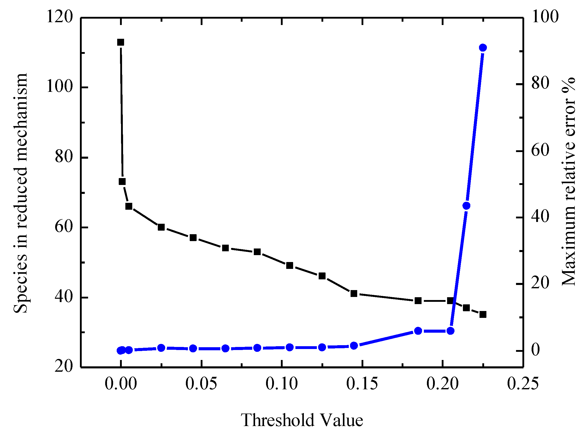
2. Mechanism Reduction

The directed relation graph with error propagation is a mechanism reduction method developed on the directed relation graph method. This method was proposed by Law C.K., in 2005, to remove the secondary components and reactions and obtain the skeletal mechanism [22,23,24].
The identification and removal of unimportant components in a detailed mechanism are quite complicated due to the mutual coupling between the components. DRG method gives an effective way to this problem. General idea of DRG is shown in Figure 1, and the first thing is to map a graph structure for the reaction system. Every species in Figure 1 denotes a vertex. If the removal of species B directly results in a significant error in the rate of formation of species A, species A is associated with species B, so A and B will be connected by an edge. And, the primary issue with the DRG method is how to define parameters to evaluate the direct impact of one species on the other. For the convenience of simplification, the DRG method does not use parameters related to the reaction system, and directly removes unimportant species by reaction mechanism analysis. The direct species A, introduced by the removal of another species B, form the mechanism. Such immediate error, noted as r A B , can be expressed as:
r A B = i = 1 , I | v A , i ω i δ B i | i = 1 , I | v A , i ω i | .
δ B i = { 1   if   the   i th   reaction   involves   species   B 0 ,   otherwise .
ω i = ω f , i ω b , i .
where A and B indicate the species, i indicates the ith reaction of the mechanism, and ν A , i indicates the stoichiometric coefficient of species A in the ith reaction. ω i , ω f , i , ω b , i represent the net reaction rate, positive reaction rate and reverse reaction rate of the ith reaction, respectively. The denominator represents the absolute contribution of all reaction mechanisms containing species A, and the numerator represents the contributions of both species A and B.
After defining the immediate error, a search begins with the target species (e.g., fuel, oxidant) selected by the user to find the relevant path of all species relative to the target species. The program iterates until it no longer has significant species to choose from, and the reduced mechanism contains only significant species and elementary reactions. When the detailed mechanism is reduced, the existence of the vertex is decided by a threshold value ( ε ), which controls the size of the reduced mechanism.
However, the standard DRG method assumes that all species retained by the mechanism are of equal importance and ignores the connection between the coupled components. If A is an initial species, and species A generates species B, and species B regenerates into species C, it is assumed that species C is as important as species B in its simplification. In DRG, if r A B is larger than the user-defined error value, species B needs to be retained. In addition, if r B C is larger than the defined error value, the species C also needs to be retained due to the coupling of species B to the A and C [25,26,27]. As can be seen, the DRG method totally neglects the longer connection way to reach species A.
To overcome this shortcoming, Pepiot–Desjardins and Pitsch proposed the concept of propagation error. In DRGEP, if species A is retained, other species can be judged by R value, which is defined as [25]:
R A B = max s { r i j } .
where S is the set of all possible paths leading from species A to species B, and r i j is the cumulative error of the given path. For example, if A is connected to B through a reaction and B is connected to C through a reaction, there is a path connecting from A to C via B and the R-value of this particular path is r A C = r A B r B C . And in Figure 1, r A E is calculated by r A E = max ( r A E d i r , r A D r D E ) . Based on this definition, a species B must be kept in the mechanism if there is at least one path connecting from A to B whose R-value is larger than the user-specified threshold, and a species C will be removed if r A C is smaller than the user-specified threshold. The test cases of the Reaction Design have shown that, under many conditions, DRGEP method can generate a skeletal mechanism that contains approximately 10% fewer species than one generated using the DRG method [28].
Not only can the ignition delay time reflect the low-temperature combustion properties, but it can also include the high temperature combustion chemistry, so the ignition delay time is selected as the parameter in mechanism reduction, and the error of the reduced mechanism are calculated as:
error r e l = | τ i g n , r e d τ i g n , det | τ i g n , det × 100 % .
where the ignition delay times of reduced and detailed mechanisms are presented as τ i g n , r e d and τ i g n , det , respectively. In this paper, the ignition delay time is defined as the time form the start to the maximum rate of temperature rise as shown in Figure 2.
In this paper, the detailed mechanism of Mech_56.54 (including 113 species and 710 reactions) developed by Curran et al. was simplified with DRGEP method using ANSYS Chemkin Reaction Workbench software (Vision 17.0, ANSYS Reaction Design, San Diego, CA, USA) [10,28]. Ignition delay times were selected as the target parameter, and the homogeneous constant volume reactor is used to solve the solution, and the solution error error r e l is controlled within 5%. The simplified temperature range is 1100–1650 K, the pressure range is 1–40 atm, and the equivalent ratio is 0.3–2.0.
From Figure 3, it can be found that with the increase of the threshold value, the size of the reduced mechanism decreases, and the maximum relative error increases. In order to get a smaller skeletal mechanism with smaller relative error, the threshold value ε is set to 0.185, and the maximum relative error ε r e l is 5.88%, and 39 species reduced mechanism was obtained. And retained species in the corresponding reduced mechanisms with different threshold value are shown in Appendix A, Table A1.

3. Verification of Reduced Mechanism

With the reduced procedure, the detailed mechanism of methane of Mech_56.54 was simplified by DRGEP method, and the reduced mechanism of 39 species and 231 reactions was obtained. The experimental data of the existing publications were simulated and compared using detailed mechanism and reduced mechanism to verify the accuracy of the mechanism.

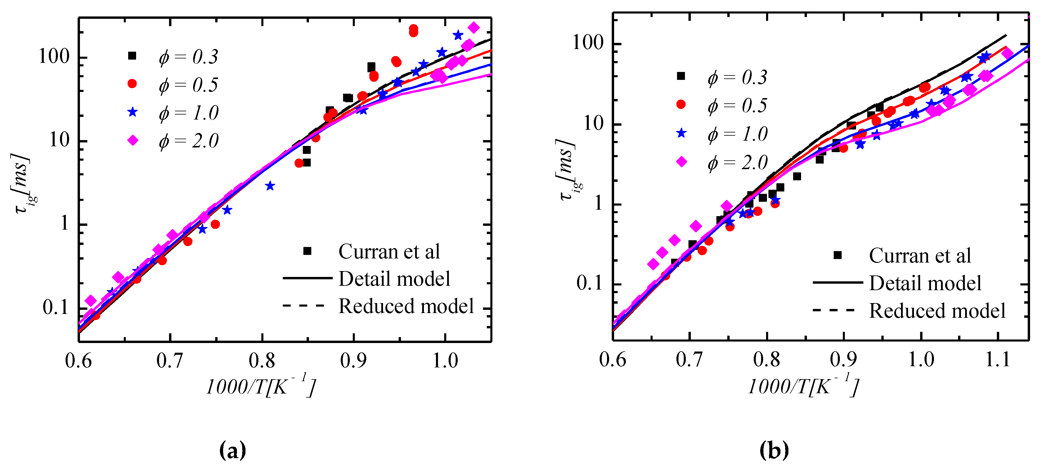
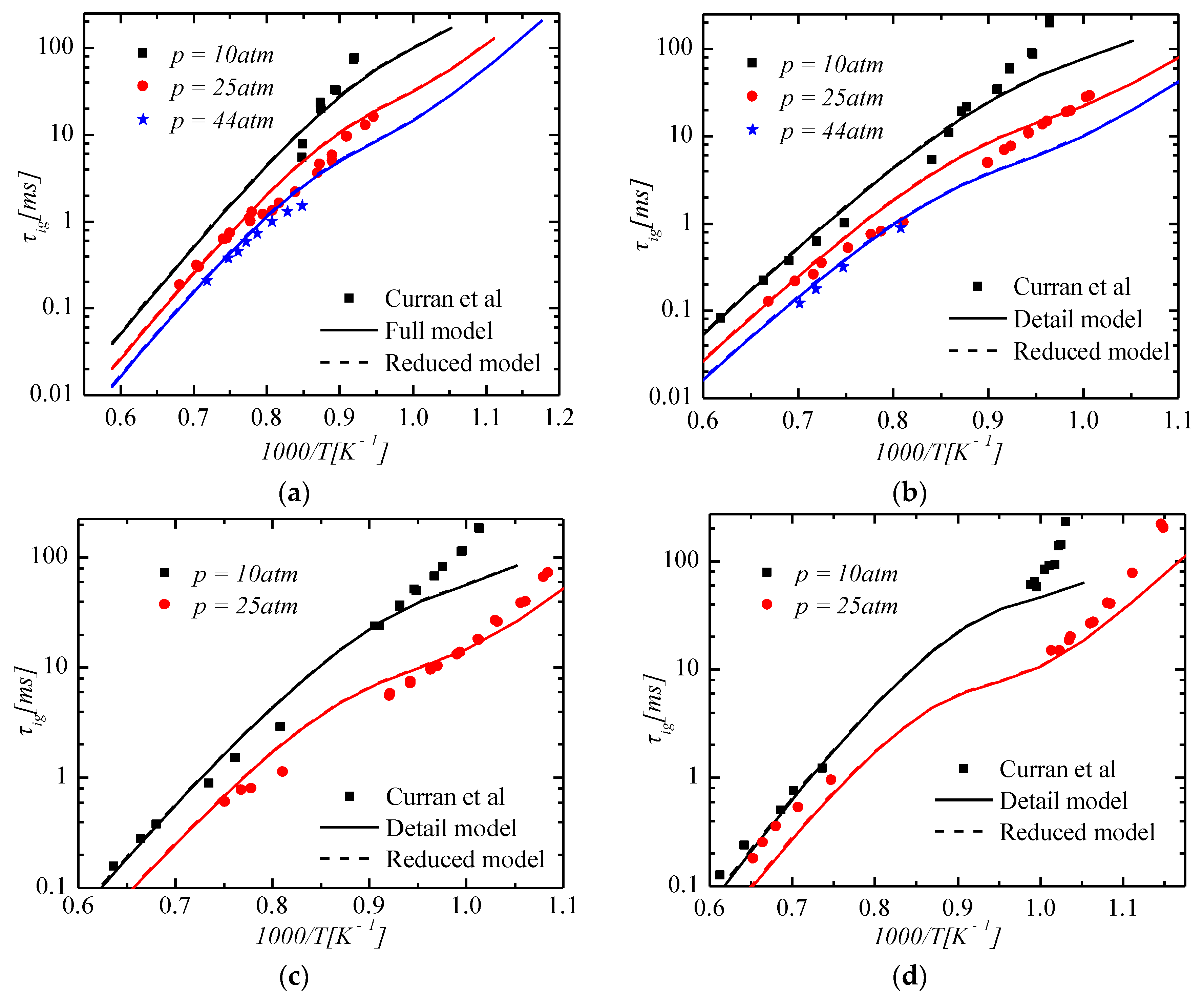
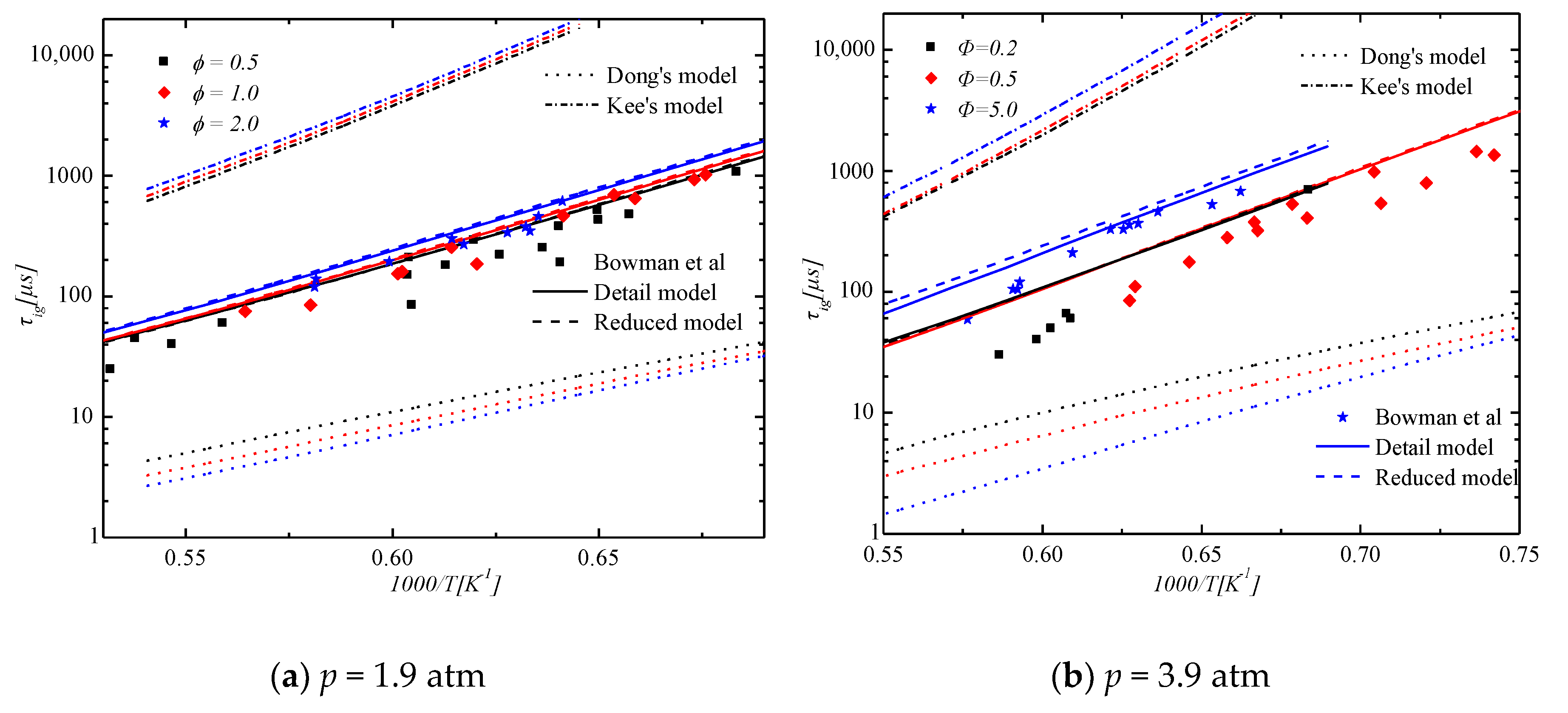
3.1. Verification of Ignition Delay Times

Ignition delay times are important attributes of fuel combustion, and they have great influence on fuel ignition, flame propagation, and development. Therefore, accurate simulation of methane ignition delay times is crucial to capture methane combustion characteristics.
In order to verify the accuracy of the reduced mechanism, the experimental data of Bowman and Curran et al. were used [10,29]. Due to the lack of heat dissipation data for the rapid compression machine, it is considered as an adiabatic process. Therefore, the simulating results will be slightly smaller than Curran’s experimental results at lower temperature. In Figure 4a,b are the ignition delay times of the CH4/O2/Ar mixture at different equivalent ratios at pressures of 1.9 atm and 3.9 atm, respectively. In these two figures, as the temperature increases, ignition delay times decrease continuously; as the equivalence ratio increase, ignition delay times increase. At high temperature conditions, the ignition delay times of CH4 change almost linearly with the reciprocal of temperature. The simulation results well capture the variation trend of ignition delay times with temperature and equivalent ratio, but there is still small error with the experimental data. In Figure 4, when equivalent ratios are smaller than 2.0, the relative errors between reduced model and full model are smaller than 4.36%. When equivalent ratio is 5.0, the relative errors become large, and the biggest relative errors are 20%. Figure 5 shows experimental data and simulation results of ignition delay times of CH4/Air mixture at different equivalent ratios at high pressures (10 atm and 25 atm). At low temperature, ignition delay times become shorter as the temperature increases. While in the middle temperature, ignition delay times are less affected by the temperature. When the temperature exceeds 1100 K, the ignition delay times are exponentially negatively correlated with the temperature reciprocal. In the low temperature range, as the equivalence ratios increase, ignition delay times decrease, which is opposite to the change in the high temperature range. Both detailed mechanism and reduced mechanism well capture the variation trend of the ignition delay times with temperature in different temperature intervals, and the errors between the reduced mechanism and the detailed mechanism are extremely small.
Figure 6 shows the effect of different pressures on the ignition delay times of the CH4/Air mixture. In Figure 6a–d, ignition delay times decrease with the increase of pressure at the equivalent ratio of 0.3/0.5/1.0/2.0, respectively. In the low temperature range, the calculation result of ignition delay times is slightly lower because the heat dissipation in the experiments of Curran et al. is not considered. In the high temperature range, all simulation results fitted the experimental results well, and the reduced mechanism is almost coincident with the detailed mechanism. This result again demonstrates that the reduced mechanism reflects well the ignition delay characteristics of CH4 over a wide range.

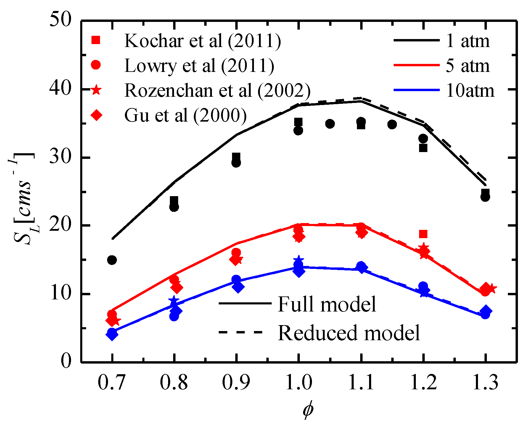
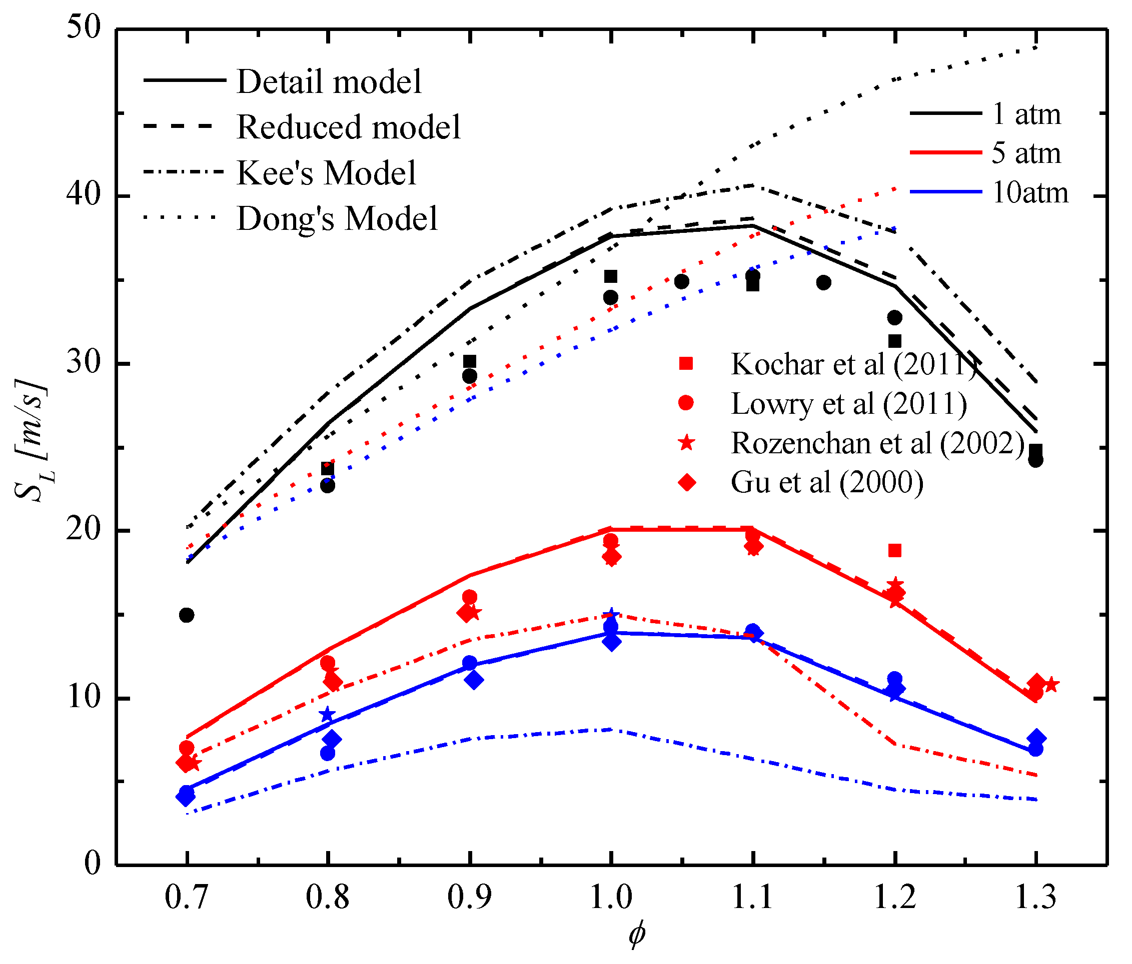
3.2. Verification of Laminar Flame Propagation Speed

As an important characteristic parameter of fuel, laminar flame propagation speed can be used to characterize the chemical reaction kinetics of fuel [30,31].
In this paper, the Laminar Flame Speed Calculation Solver of the Chemkin software (Vision 17.0, ANSYS Reaction Design, San Diego, CA, USA) was used to calculate the propagation speed of the CH4/Air mixture. The laminar flame propagation speed of CH4 at different pressures is shown in Figure 7, wherein the temperature of the unburned mixture is 298 K. At the same pressure condition, the flame propagation speed of CH4 increases first and then decreases with the increase of the equivalence ratios, and reaches a peak value between the equivalent ratio of 1–1.1. When the pressure is low, the flame propagation speed between different equivalent ratios varies greatly, while when the pressure is high, the difference is small. The solid line and the dashed line in Figure 7 represent the calculated results of the detailed mechanism and the reduced mechanism, respectively. The simulated curve accurately captures the change in the laminar flame propagation speed of CH4 as a function of pressures and equivalence ratios. At all equivalent ratios and pressures conditions, the results calculated by the reduced mechanism and the detailed mechanism have little error and are very close to the experimental results [32,33,34,35]. Average relative error between reduced model and full model of all conditions is 0.88%, and the biggest relative error between two models is 2.99%.

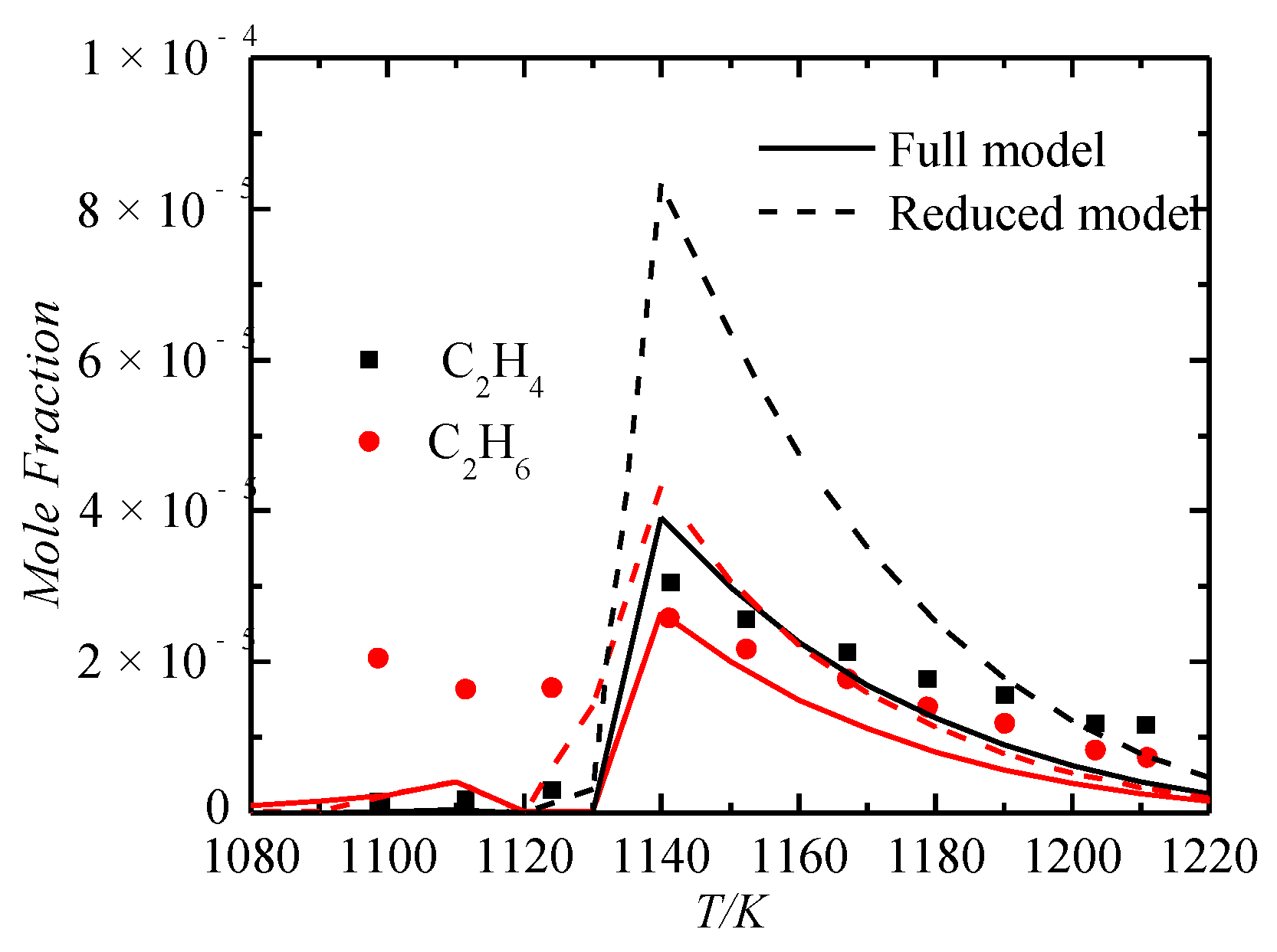
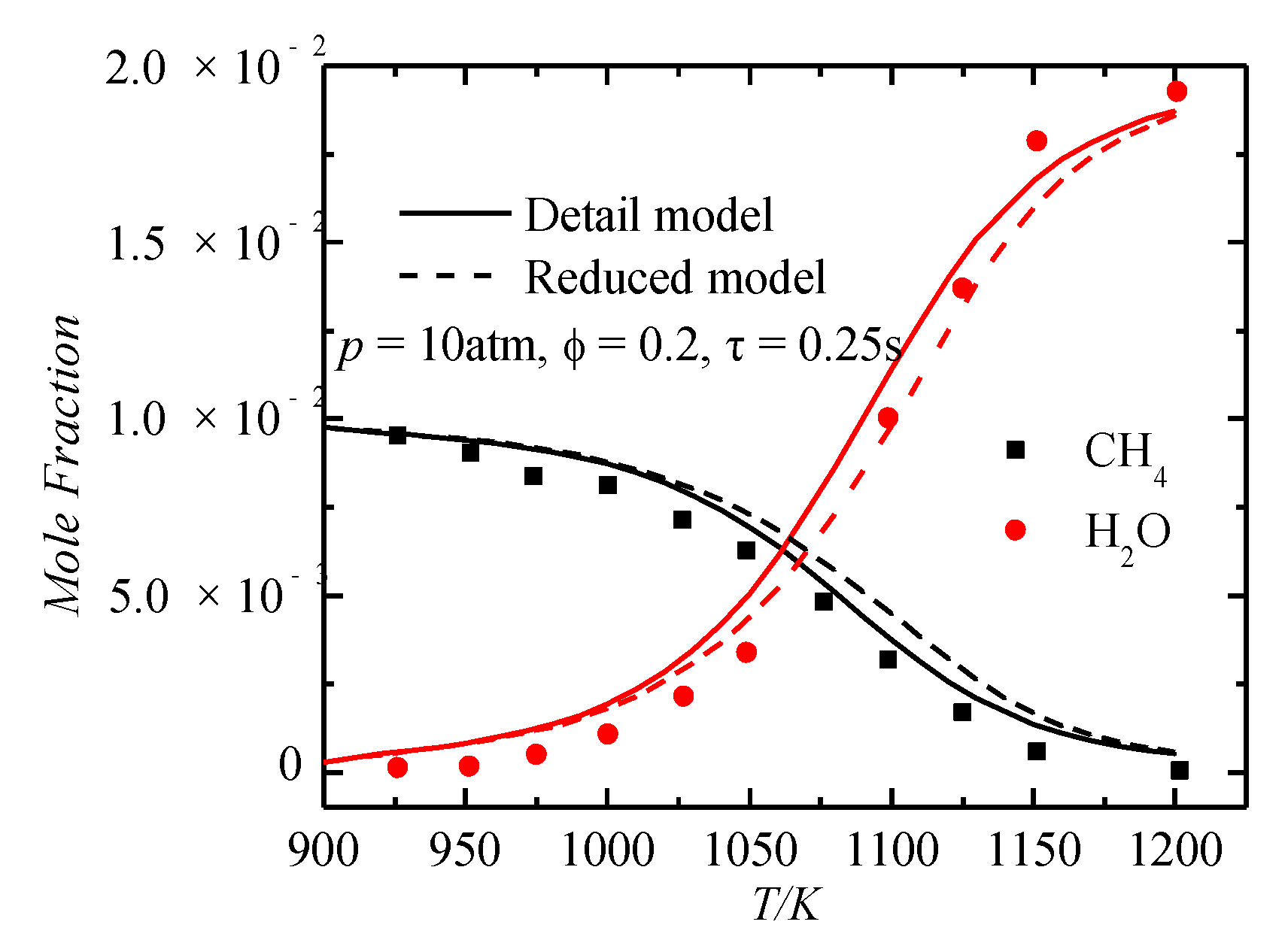
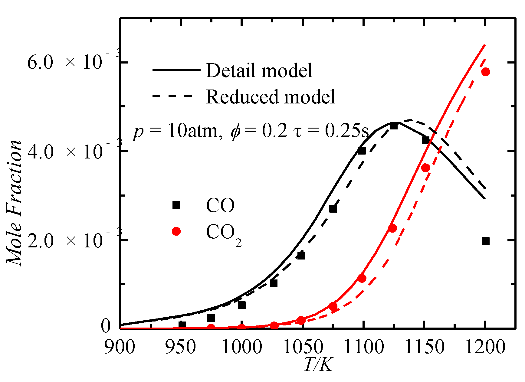
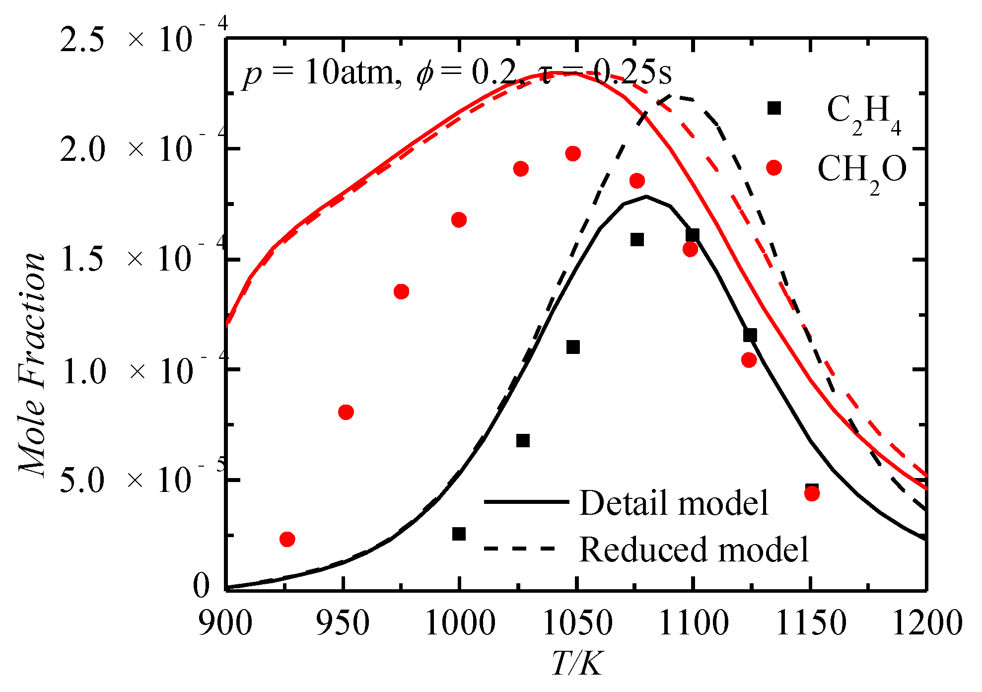
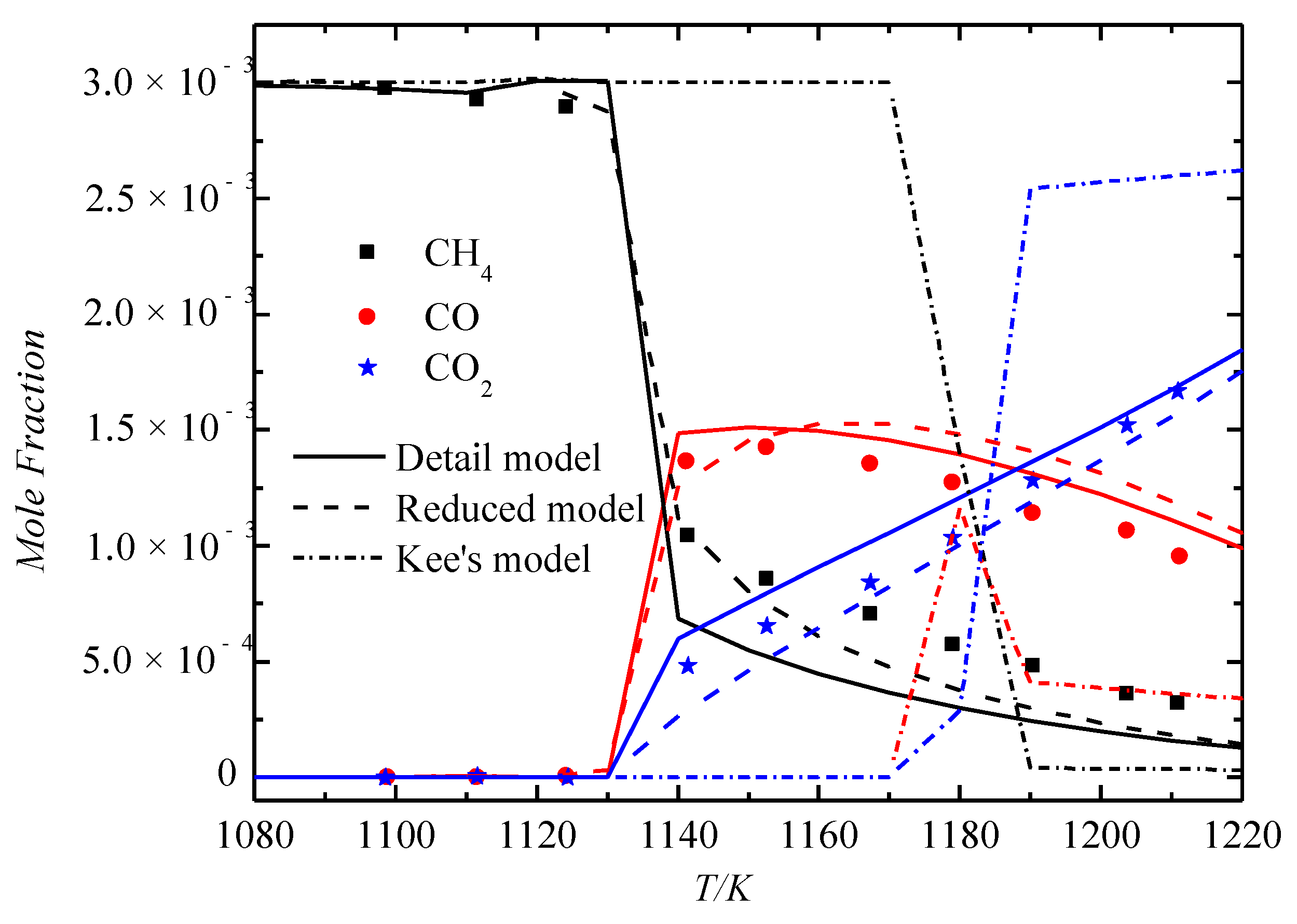
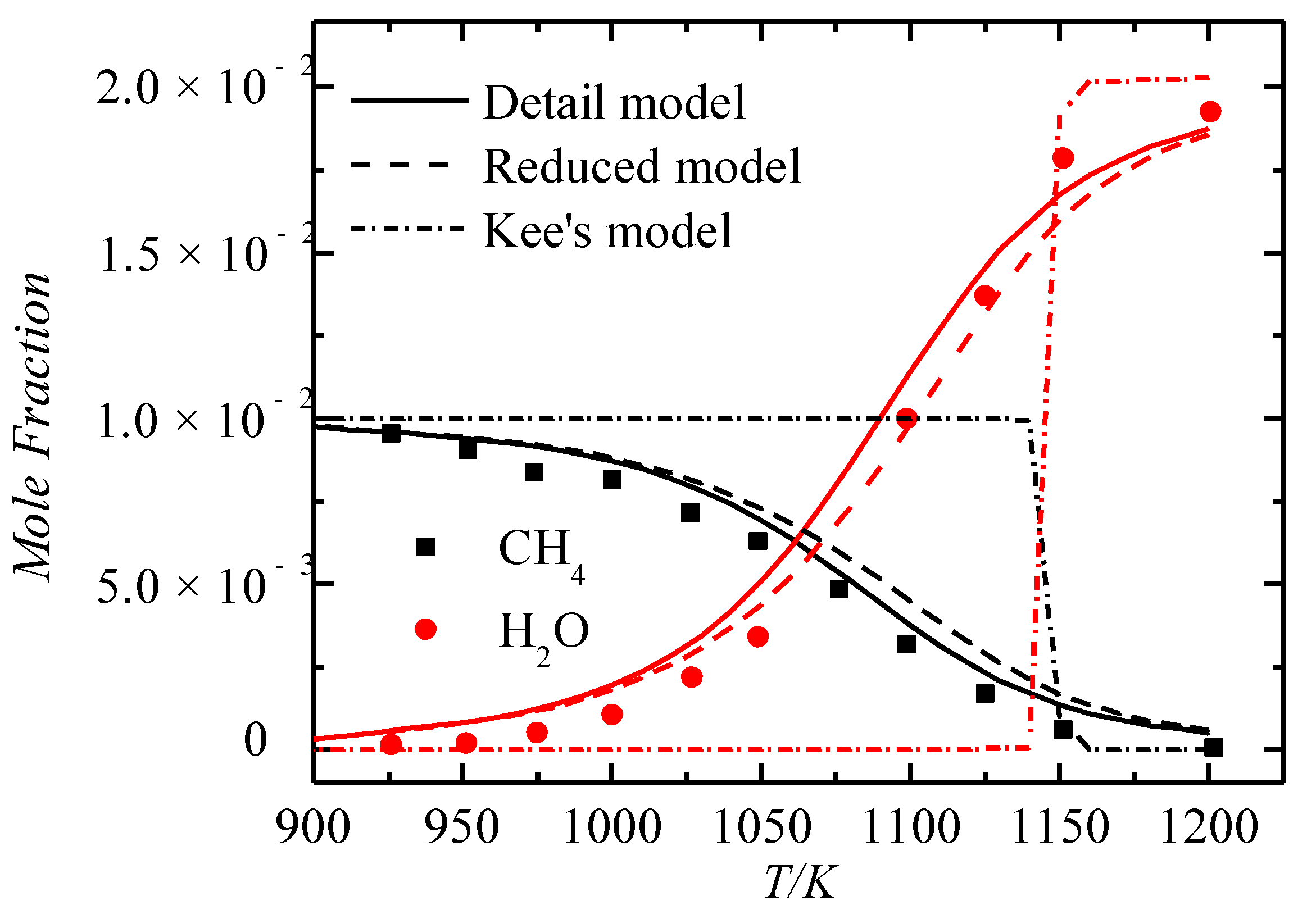
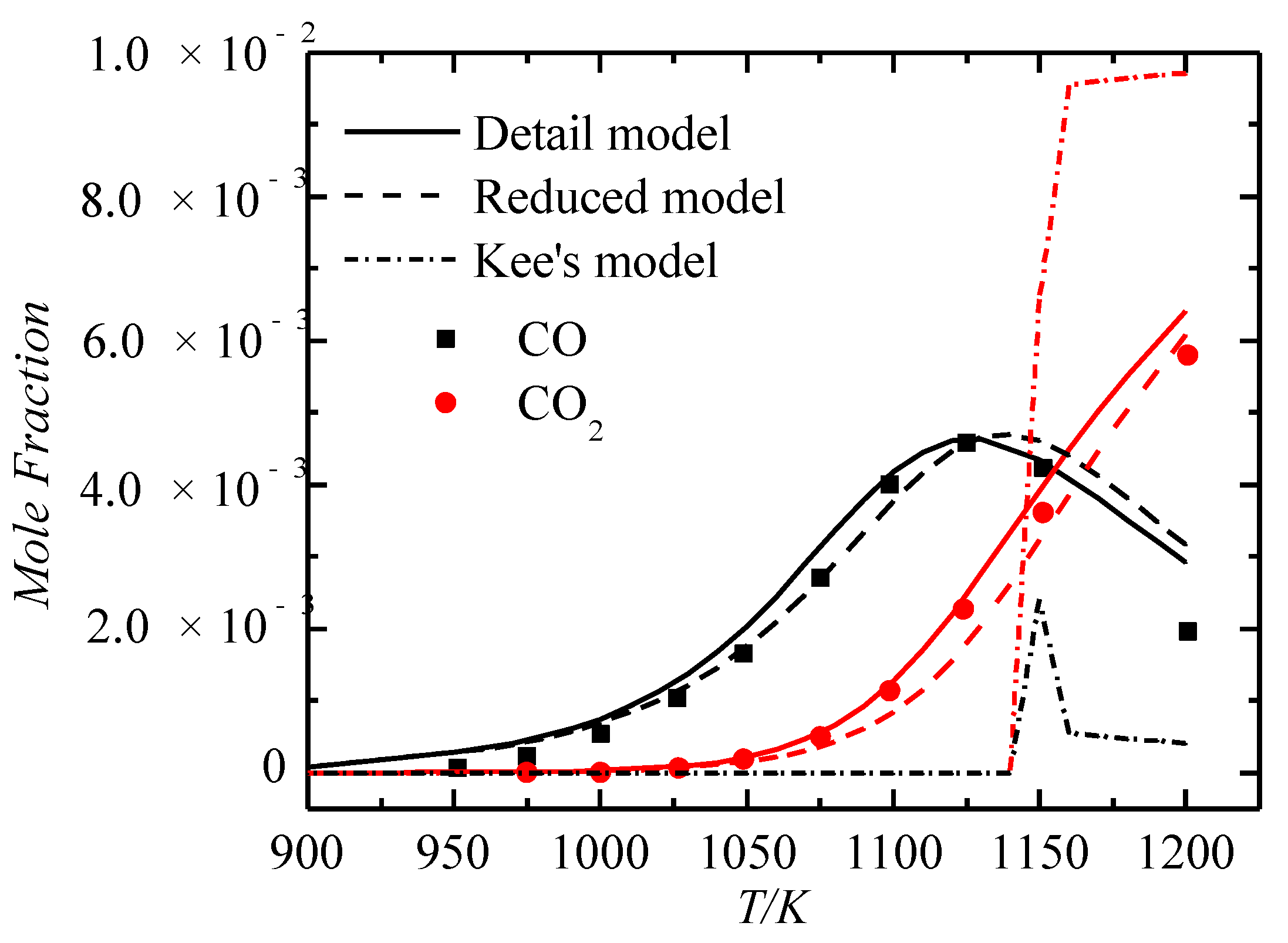
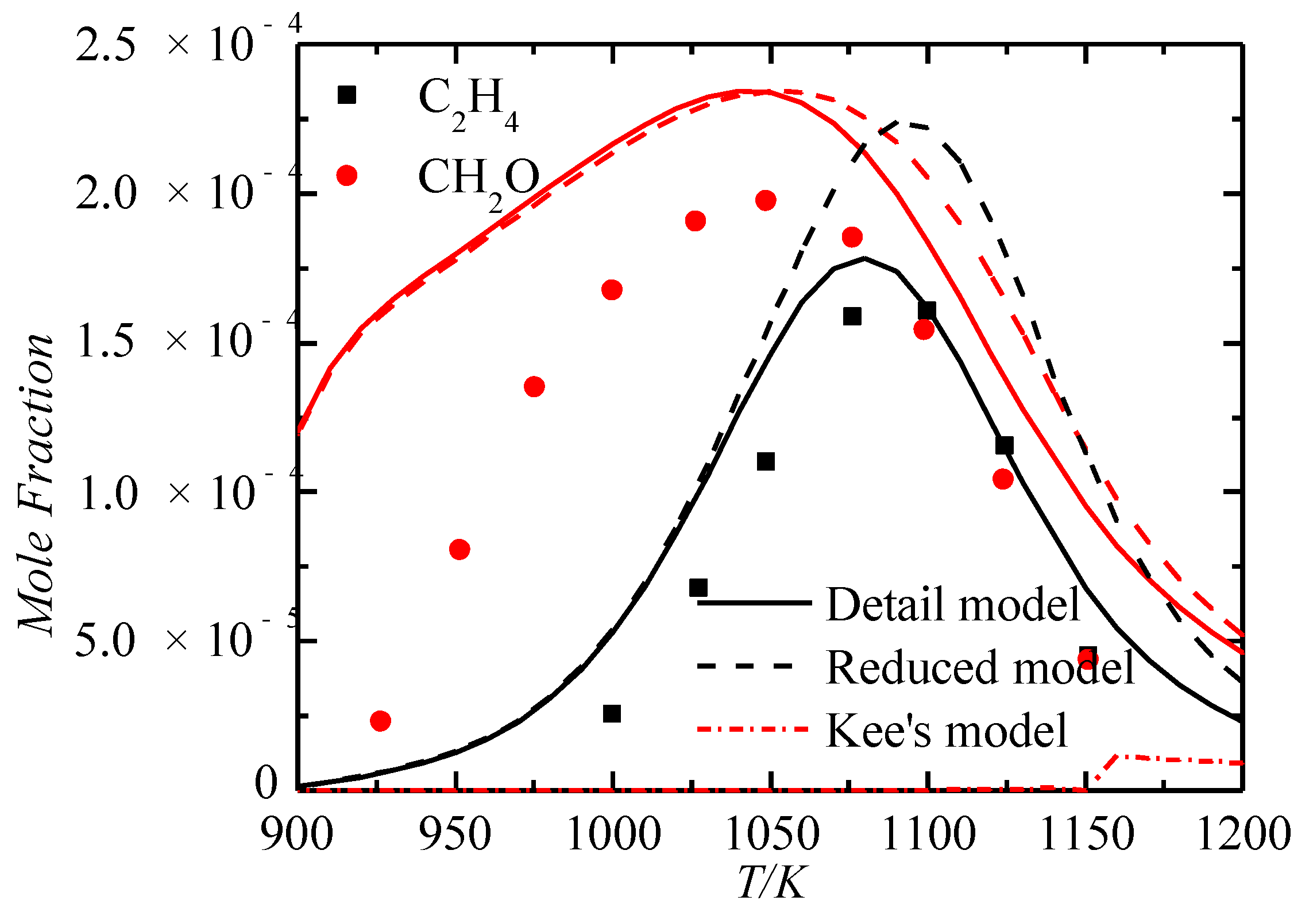
3.3. Verification of Important Species

In order to further verify the accuracy of the mechanism, the experimental data of the jet-stirred reactors of Dagaut et al. and Lecong et al. were simulated and compared using a reduced mechanism and a detailed mechanism [36,37]. In the Dagaut’s experiment, the proportion of CH4/O2/N2 at 1 atm was 0.3%/6%/93.7%, and the residence time was 0.1 s. The species concentration distribution of the CH4/air mixture at different temperatures is shown in Figure 8. As can be seen from the figure, the concentration of CH4 gradually decreases with the increase of temperature, while the concentrations of CO and CO2 keep increasing. Figure 9 shows the intermediate product of CH4/air mixture. At approximately 1140 K, the concentrations of C2H4 and C2H6 reach a maximum, and then the concentrations decrease as the temperature increased. Detailed mechanism and reduced mechanism can simulate well the trend of formation and consumption of important components in combustion. For relatively stable components, such as CH4/CO/CO2, the error between simulation results and experimental values is small. And for the intermediate component C2H4, the simulation results of the reduced mechanism are slightly larger. C2H4 is consumed by reaction C2H4 + H + M = C2H5 + M in both reduced mechanism and detailed mechanism. However, the producing rate of C2H4 is bigger than the consumption rate of C2H4 in detailed mechanism, so the mole fraction of C2H4 is small. While, the producing rate of C2H4 is even smaller than the consumption rate of C2H4 in reduced mechanism, so the mole fraction of C2H4 is relatively large.
The discrete points in Figure 10, Figure 11 and Figure 12 are experimental data obtained by Lecong et al. using a jet stir reactor. The solid and dashed lines are the results of a detailed mechanism and a reduced mechanism, respectively [37]. In the experiment, pressure of 10 atm, equivalent ratio of 0.3, and residence time of 0.25 s were selected. In this experiment, the variations of components are similar to those in Figure 8 and Figure 9. The reactants are continuously consumed as the temperature increases, and the products accumulate continuously, and the concentrations of the intermediate products first increase and then decrease. Compared with the experiment when the pressure was 1 atm and the equivalent ratio was 0.1, the components change relatively slowly at each temperature. It can be seen from the figure that both the simulation results and the experimental results can well capture the variation characteristics of each component at different temperatures. For the intermediate components, such as CH2O and C2H4, the errors are relatively large, and all the other components are in good agreement.
In order to make the reduced mechanism analysis more effective, the reduced mechanism is also compared with other mechanisms, as shown in Appendix B.

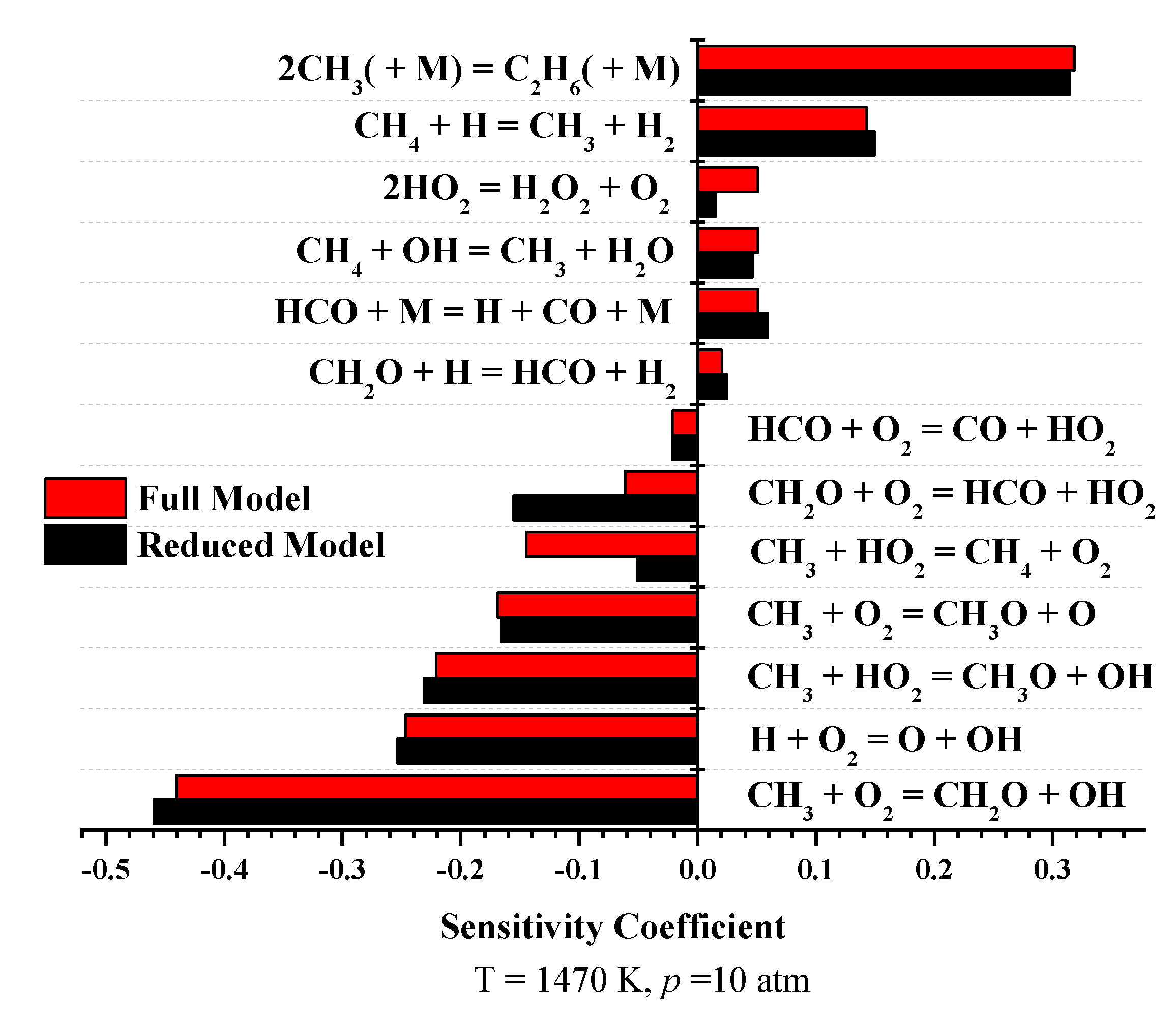
4. Sensitivity Analysis

Sensitivity analysis is of great significance to understand the key reactions and mechanism simplification of chemical reaction kinetics of fuel combustion [38]. In order to find the important reaction to control the ignition in methane combustion, it is necessary to analyze sensitivity of the ignition delay times. In general, the sensitivity coefficient (S) can be expressed by the following equation:
S = l n ( τ + τ ) l n ( k + k ) = ln ( τ + τ ) ln ( 2.0 0.5 ) .
When the sensitivity coefficient (S) is negative, the reaction is the promoting reaction (the ignition delay time will be reduced with the increase of pre-exponential factor). When the sensitivity coefficient (S) is positive, the reaction is an inhibitory reaction (the ignition delay will increase with the increase of pre-exponential factor increases) [10].
As shown in Figure 13, it is the sensitivity analysis of the ignition delay times of the detailed mechanism and the reduced mechanism of the CH4/Air stoichiometric mixture at 1470 K and pressure 10 atm. As can be seen from the figure, C H 3 + O 2 = C H 2 O + O H promotes the combustion of CH4, which rapidly converts CH3 produced by the pyrolysis of CH4 into CH2O and OH radical. For the 2 C H 3 ( + M ) = C 2 H 6 ( + M ) reaction, CH3 radicals are combined to form ethane, which reduces the reaction rate and therefore inhibits the reaction. It can be seen from Figure 13 that the formation of small molecule active radicals (HO2/O/OH) usually promotes the ignition, while the reaction of consumption of active radicals and the formation of relatively stable components is usually not conducive to ignition. From the figure, we can find that the analysis results of the reduced mechanism are basically identical with the detailed mechanism, with only minor differences in the sensitivity coefficients of partial reactions.

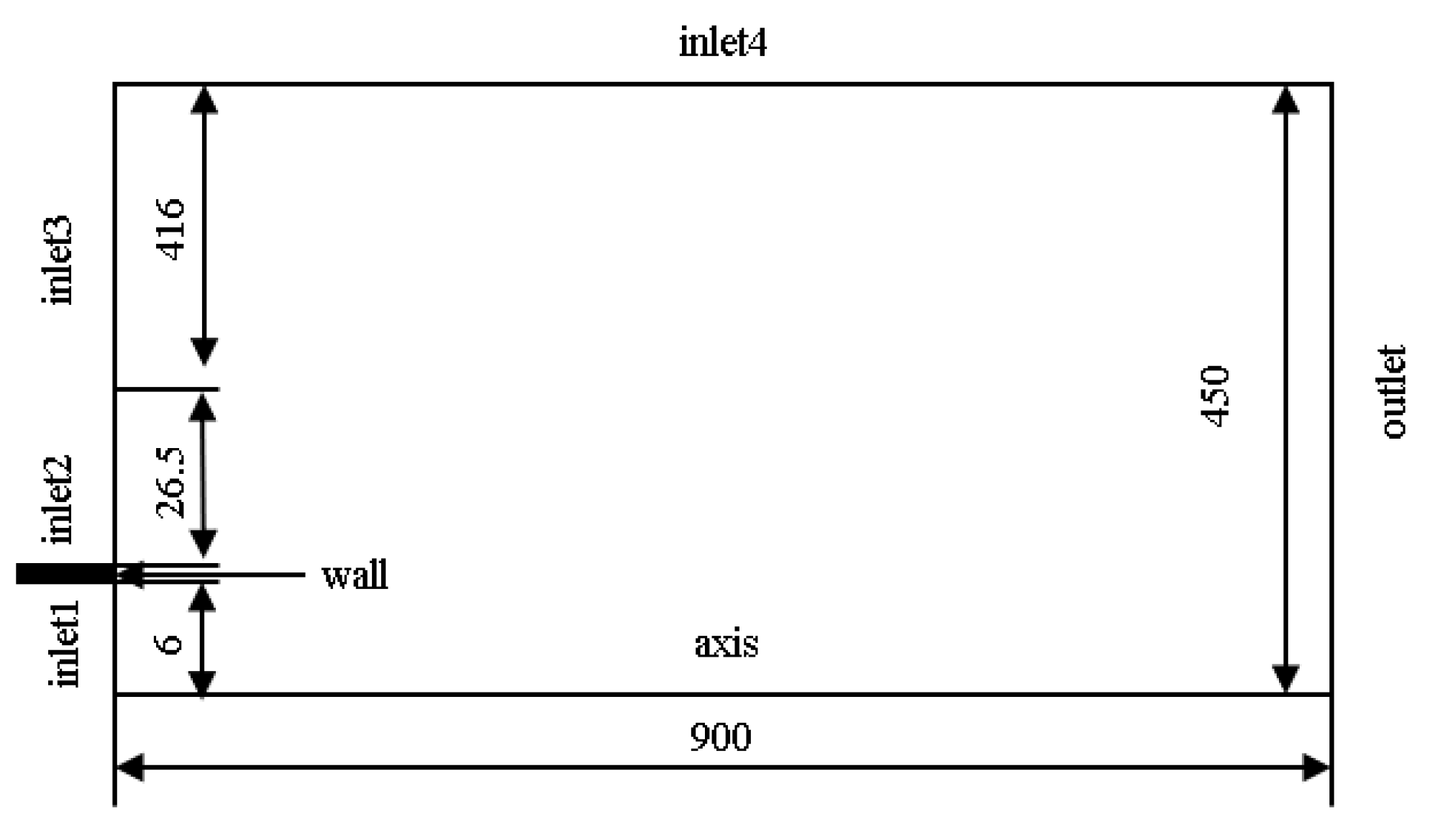
5. Flame Simulation and Verification of Bunsen Burner

In order to further verify the reduced mechanism, the Bunsen burner premixed flame was simulated using a two-dimensional model and compared with the experiments of Chen Y.C. et al [39]. The calculating geometry is shown in Figure 14. The diameter of inlet 1 is D = 12 mm, the average inlet velocity is u 0 = 50 m / s , the average turbulent energy is k 0 = 10.8 m 2 / s 2 , and the Reynolds number is 40,000. In the experiment, gases of the inlet 1 are CH4/Air stoichiometric mixture and the temperature was 298 K. The gases of the inlet 2 are burned gases, the temperature is 1900 K, and the gases of inlet 3 and the inlet 4 are air. During the simulation, the boundary conditions of the inlet are given according to the experimental measurement data given the velocity and the turbulent energy, and the outlet is the pressure boundary condition. The calculation domain is 900 mm × 450 mm , and the independence of the grid is verified during simulation. The software ANSYS FLUENT ( Version 17.0, ANSYS Inc, Pittsburgh, PA, USA.) was used for simulation, and the eddy-dissipation-concept model (referred to as EDC model) was selected [40]. The EDC model can simulate the turbulent-chemical kinetic interaction using a detailed chemical reaction mechanism with high simulation accuracy [41].

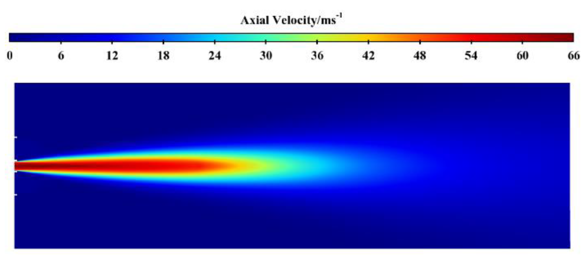
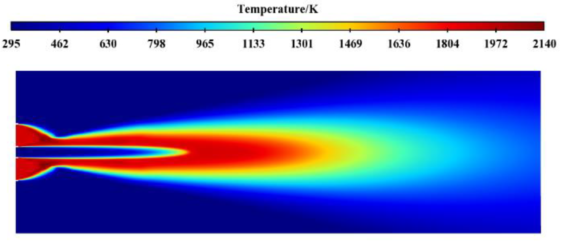
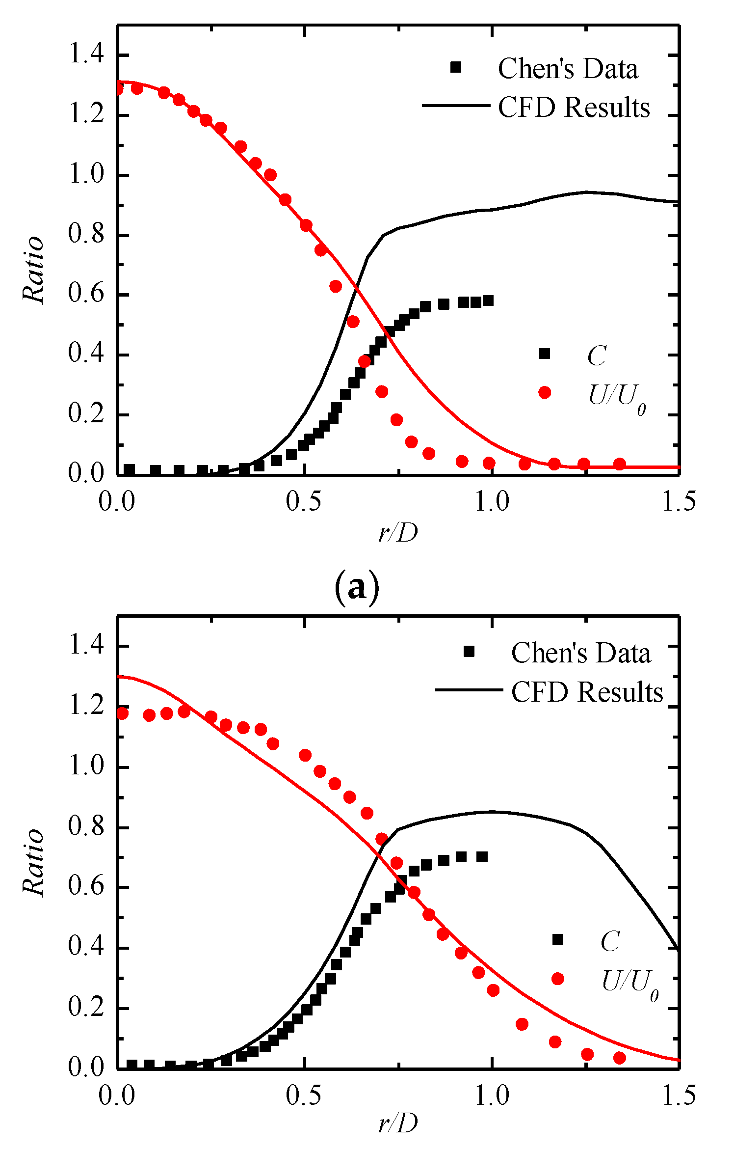
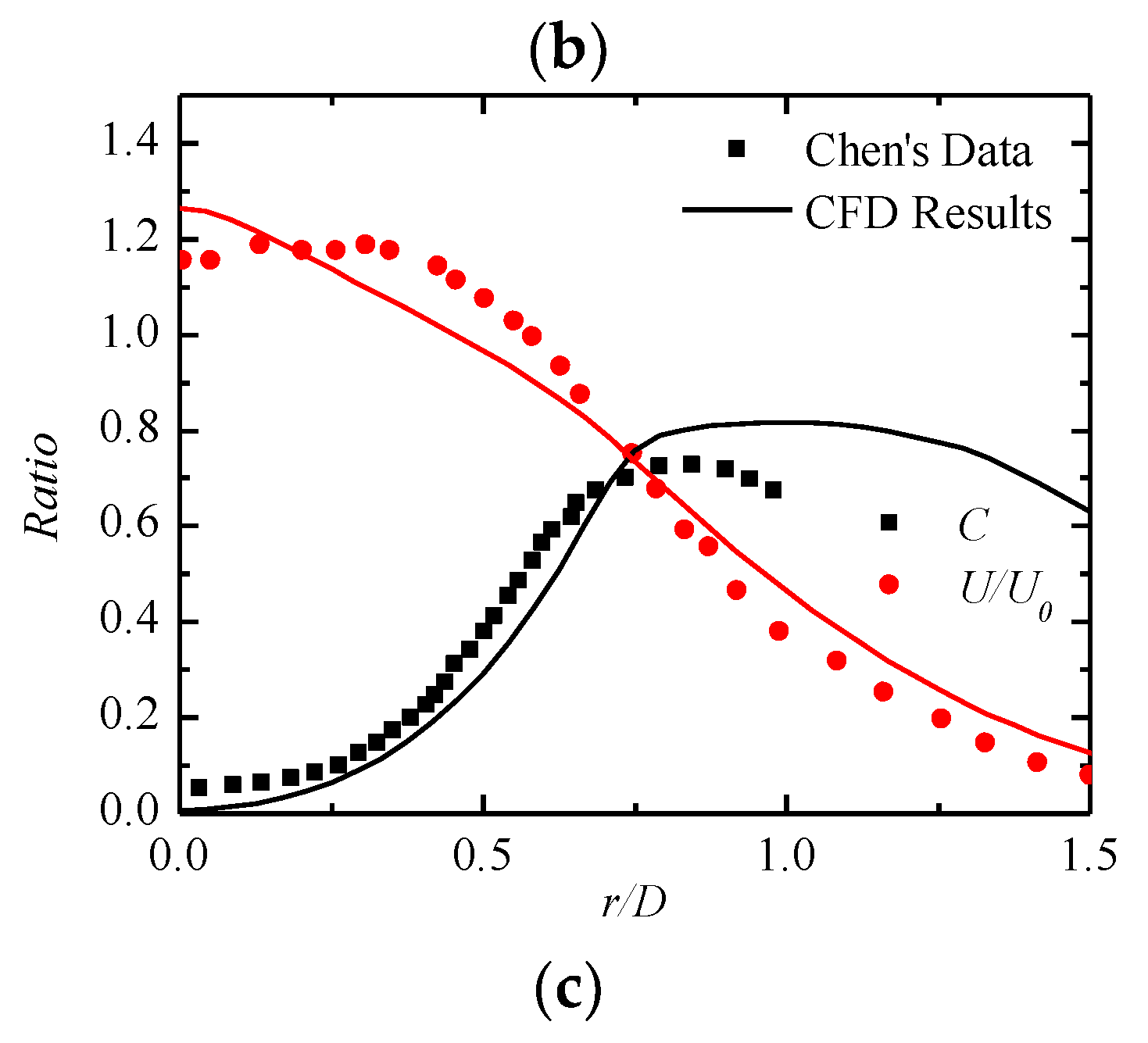
5.1. Comparison of Axis Velocity and Temperature

In order to better show the simulation results, the contour image of the simulation results is symmetrically processed. Figure 15 shows the axial velocity distribution of the Bunsen burner flame. The airflow expands slightly outward after flowing through the outlet, and the axis velocity gradually decreases with the increase of jet depth. Figure 16 shows the contour of flame temperature distribution of Bunsen burner. Outside the outlet of the premixed gas, the surrounding temperature is around 1900 K, and the temperature in the downstream gradually increases due to the heat release caused by chemical reaction. The flame temperature is lower in the downstream of the air outlet due to the larger velocity, but the flame temperature increases rapidly when it reaches the reaction zone.
In order to quantitatively compare the calculated values with the experimental results, three axial positions (X/D = 2.5, X/D = 4.5, and X/D = 6.5) are selected for analysis. The axial velocity is dimensionless using the average velocity U 0 , and the dimensionless temperature is defined as C = ( T ~ T u ) / ( T b T u ) , where K and T u = 298 K .
Figure 17 shows the comparison of the dimensionless axial velocity and the dimensionless temperature with the experimental results of different axial positions. The solid points are experimental results of Chen Y.C. et al., and the lines are the calculation results. As can be seen from Figure 17a, when r/D < 0.5, the calculated values of axial velocity almost coincide with the experimental values, while when r/D is between 0.5 and 1.1, the calculated results are slightly larger than the experimental values. In Figure 17b,c, when r/D > is 0.75, the simulation results are slightly larger than the experimental values, while at r/D < 0.75, the simulation results are slightly smaller than the experimental results. In the three graphs, the dimensionless temperature values are basically the same as the distribution trend of the experimental results. With the increase of r/D, the values increase first and then decrease. At X/D = 2.5, the dimensionless temperature error was the largest, followed by X/D = 4.5 and X/D = 6.5 is the smallest. This is mainly because the adiabatic model is adopted in the simulation calculation without considering the influence of heat dissipation at the inlet, which makes the calculation temperature high. As the axial position increases, the influence of the non-adiabatic effect of the inlet becomes smaller, making the calculation result more accurate.

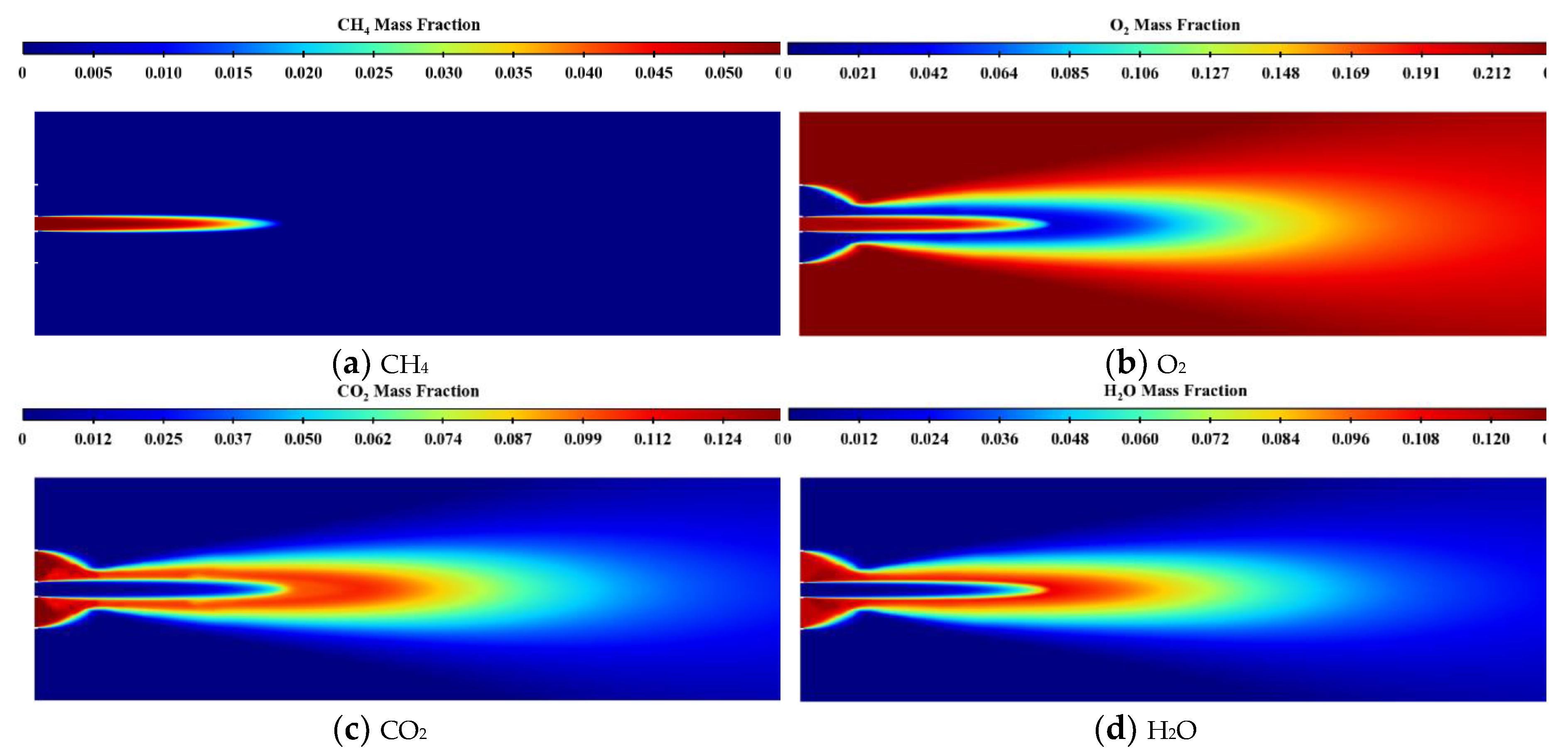
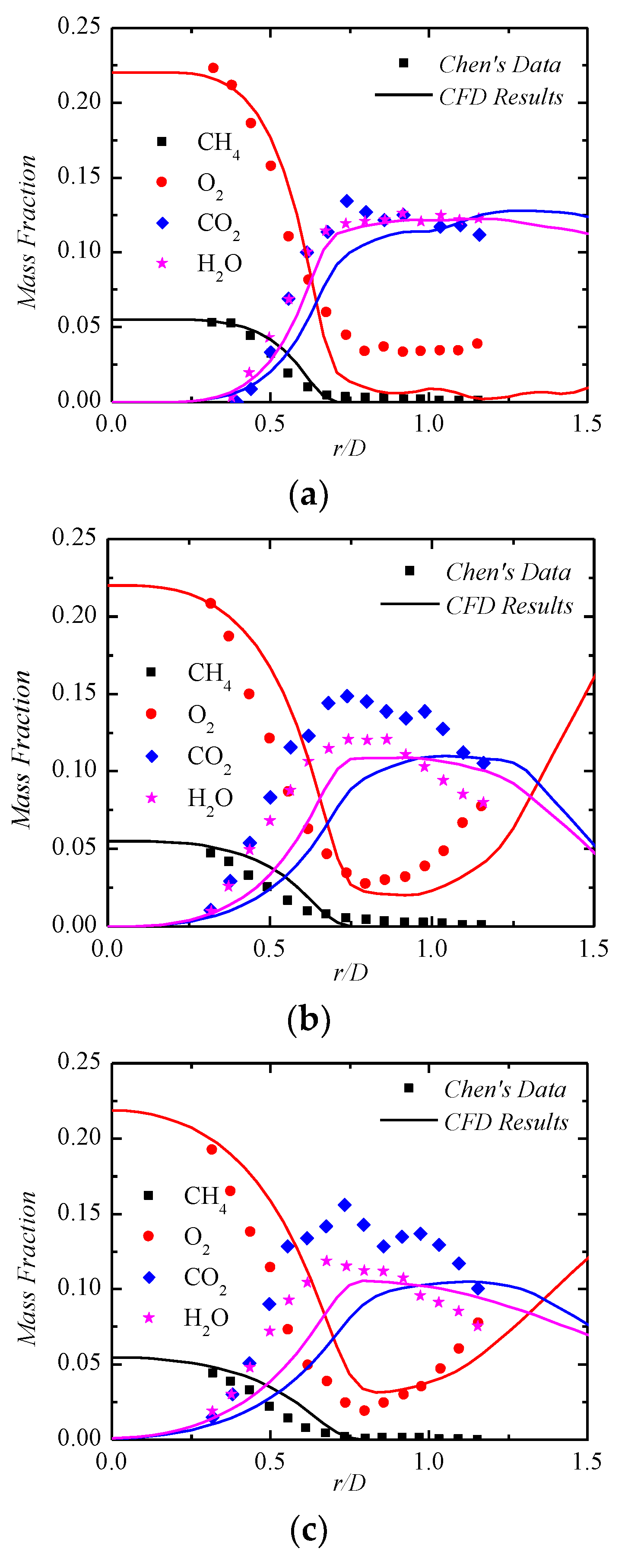
5.2. Comparison of Important Species

Figure 18 shows the distribution of significant species of Bunsen burner flame, and Figure 18a shows the mass fraction distribution of CH4. As the depth of the jet increases, the concentration of CH4 decreases continuously. This distribution is similar to the axial velocity in Figure 15, but the distribution is narrower than the axial velocity and presents a tendency to converge continuously. In Figure 18b, since the CH4/Air mixture is a stoichiometric premixed gas, the oxygen concentration in the jet is high. In the reaction zone, as the chemical reaction occurs, the oxygen concentration gradually decreases, and the concentration of oxygen in the active reaction zone is almost zero. It can be seen from Figure 18c,d that a large amount of H2O and CO2 are generated in the active reaction zone.
Figure 19 shows the distribution of important species in different axial positions of Bunsen burner flame, and the simulation results in all locations perfectly capture the CH4 consumption. At the same time, when r/D < 0.75, the change of oxygen concentration with radius is also consistent with the experiment; Since the heat dissipation at the outlet wall is not considered, the oxygen concentration is closer to the experiment as the axial position increases at r/D > 0.75; at X/D = 2.5, CO2 and H2O are in good agreement with the experimental results, while at X/D = 4.5 and 6.5, the overall change trend is basically consistent with the experimental results, but there is a certain error in the numerical value.
By using the reduced mechanism to simulate the premixed flame of Bunsen burner, the reduced mechanism can well capture the combustion characteristics of CH4/Air premixed flame and truly reproduce the distribution of combustion flow field, temperature field and important species in the experiment.
Authors should discuss the results and how they can be interpreted in perspective of previous studies and of the working hypotheses. The findings and their implications should be discussed in the broadest context possible. Future research directions may also be highlighted.

6. Conclusions

Based on the DRGEP method, the detailed mechanism of Mech_56.54 methane developed by Curran et al. was systematically simplified, and finally a reduced mechanism with 39 species and 231 reactions was obtained. Using the current published experimental data, the methane ignition delay times, laminar flame propagation speed, and important components obtained by the reduced mechanism were compared and verified. The simulation results of this mechanism are in good agreement with the experimental results. The Bunsen burner flame was simulated by the reduced mechanism. The calculation results show that errors of the dimensionless temperature and dimensionless velocity are extremely small between simulation and experimental data, and the distribution of important species are basically consistent with the experiment, indicating that the mechanism can be applied to CFD simulation accurately.

Author Contributions

Conceptualization, H.L., F.L., C.L., G.X., and Y.W.; methodology, H.L., X.F., Y.W., and J.H.; software, H.L., Y.W., and J.H.; Validation, H.L., X.F., F.L., and G.X.; Formal Analysis, H.L.; Investigation, H.L.; Resources, F.L. and G.X.; Data Curation, G.X.; Writing—Original Draft Preparation, H.L.; Writing—Review and Editing, H.L.; F.L., and C.L.; Visualization, H.L. and C.L.; supervision, F.L. and G.X.; Project Administration, G.X.; Funding Acquisition, J.H.

Funding

This research was funded by the National Natural Science Foundation of China, grant number 51806219.

Conflicts of Interest

The authors declare no conflict of interest.

Appendix A

Table A1. Retained species in the corresponding reduced mechanisms with different threshold value.
Threshold value (ε)SpeciesDifferent Species
0113Ar, HOCH2O2H, O2CH2CHO, CH3CO3H, CH3CO3, CH3CO2, C2H5OH, SC2H4OH, O2C2H4OH, CH3COCH3, CH3COCH2O2, C3KET21, C2H5CHO, C2H5CO, CH3OCH2, CH3OCH2O2, CH2OCH2O2H, CH3OCH2O2H, CH3OCH2O, CH3OCHO, CH3OCO, CH2OCHO, He, C3H6OOH1-2, C3H6OOH1-3, CC3H4, CJ*CC*CC*O, C*CC*CCJ*O, CJ*CC*O, C*CC*CCJ, C*CC*CC, C*CC*CCOH, HOC*CC*O, HOC*CCJ*O, HOCO
0.00178C2H2OH, HO2CH2CO, PC2H4OH, C2H4O2H, CH3COCH2, C2H3CHO, O2CH2OCH2O2H, HO2CH2OCHO, OCH2OCHO, HOCH2OCO, C3H8, IC3H7, NC3H7, C3H6, C3H5-A, C3H5-S, C3H5-T, C3H5O
0.02560HOCH2O2, C, CH3CO, C2H5O2H, C2H5O2, C2H4O1-2, C2H3O1-2, C2H3CO, C3H4-P, C3H4-A, C3H3, H2CC, H2CCC(S), C#CC*CCJ
0.12546OCH2O2H, CH*, C2H, CH3CHO, C2H3OH, CH2CHO, C2H5O
0.18539H, H2, O, O2, OH, OH*, H2O, N2, HO2, H2O2, CO, CO2, CH2O, HCO, HO2CHO, HCOH, O2CHO, HOCHO, OCHO, HOCH2O, CH3OH, CH2OH, CH3O, CH3O2H, CH3O2, CH4, CH3, CH2, CH2(S), CH, C2H6, C2H5, C2H4, C2H3, C2H2, CH2CO, HCCO, HCCOH, CH3OCH3

Appendix B: Comparison of the Reduced Mechanism with Other Simplified Mechanisms

In order to make the reduced mechanism analysis effective, the reduced mechanism is compared with other mechanisms. Since many simplified mechanisms cannot be obtained directly from the literature, authors chose two mechanisms which are contained in literature. Dong et al. adopted genetic algorithm to simplify the GRI-MECH 3.0 mechanism with the component concentration as the goal, and finally obtained the 17 species and 24 steps reaction mechanism [42]. Kee et al. proposed a 17 species and 58 steps reaction mechanism. Ignition delay times, laminar flame speed and important species are compared with these mechanisms [43].

Comparison of Ignition Delay Times

As can be seen in Figure A1, results of Dong’s model is smaller than experimental data and results of Kee’s model is larger than experimental data. And results of the reduced model are in good agreement with results of the full model and experimental data. In Dong’s model, with the increase of the equivalent ratios, ignition delay times decrease, this phenomenon is different from experimental data and other models.
Figure A1. Influence of equivalent ratios on ignition delay times of CH4/O2/Ar mixture. Solid line shows results of the full model, dash line shows results of the reduced model, dot line shows results of Dong’s model, short dash dot line shows results of Kee’s model, and discrete point shows experimental data from [29]. (a) p = 1.9 atm and ϕ = 0.5, 1.0, and 2.0 in black, red, and blue, respectively; (b) p = 3.9 atm and ϕ = 0.2, 0.5, and 5.0 in black, red, and blue, respectively. Not all data are visible due to overlapping profiles.
Energies 12 00097 g0a1

Comparison of the Laminar Flame Propagation Speed

As can be seen in Figure A2, when p = 1 atm, equivalent ratios are smaller than 1.1, all models can capture changes of laminar flame speed with the increase of equivalent ratios. There are great errors in Dong’s model when equivalent ratios are larger than 1.1. When p = 5 atm or p = 10 atm, both Kee’s model and Dong’s model have great errors with experimental data. Overall, the reduced model by authors are in good agreement with experimental data and full model.
Figure A2. Influence of pressure on laminar flame speed of CH4/Air mixture. Solid line shows results of the full model, dash line shows results of the reduced model, dot line shows results of Dong’s model, short dash dot line shows results of Kee’s model and discrete point shows experimental data from [32,33,34,35]. Kochar et al.’s data are shown as square points; Lowry et al.’s data are shown as circle points; Rozenchan et al.’s data are shown as star points; and Gu et al.’s data are shown as diamond points.
Energies 12 00097 g0a2

Comparison of Important Species

Since big differences between Dong’s model and experimental data, results of Dong’s model are not shown in Figure A3, Figure A4, Figure A5 and Figure A6, when comparing the important species. For relatively stable components, such as CH4/CO/CO2, results of reduced model and full model can well match with experimental data, however results of Kee’s model doesn’t even show the trend. For the intermediate component of CH2O, results of Kee’s model are totally different from experimental data.
Figure A3. Mole fraction of CH4/CO/CO2. p = 1 atm, ϕ = 0.1, and τ = 0.1 s. Solid line shows results of the full model, dash line shows results of the reduced model, short dash dot line shows results of Kee’s model, and discrete point shows experimental data from [36]. CH4 mole fraction is shown in black and; CO mole fraction is shown in red; and CO2 mole fraction is shown in blue.
Energies 12 00097 g0a3
Figure A4. Mole fraction of CH4/H2O. p = 10 atm, ϕ = 0.3, and τ = 0.25 s. Solid line shows results of the full model, dash line shows results of the reduced model, short dash dot line shows results of Kee’s model, and discrete point shows experimental data from [37]. CH4 mole fraction is shown in black and H2O mole fraction is shown in red.
Energies 12 00097 g0a4
Figure A5. Mole fraction of CO/CO2. p = 10 atm, ϕ = 0.3, and τ = 0.25 s. Solid line shows results of the full model, dash line shows results of the reduced model, short dash dot line shows results of Kee’s model, and discrete point shows experimental data from [37]. CO mole fraction is shown in black and CO2 mole fraction is shown in red.
Energies 12 00097 g0a5
Figure A6. Mole fraction of C2H4/CH2O. p = 10 atm, ϕ = 0.3, and τ = 0.25 s. Solid line shows results of the full model, dash line shows results of the reduced model, short dash dot line shows results of Kee’s model, and discrete point shows experimental data from [37]. C2H4 mole fraction is shown in black and CH2O mole fraction is shown in red.
Energies 12 00097 g0a6

References

  1. Molino, A.; Nanna, F.; Migliori, M.; Iovane, P.; Ding, Y.; Bikson, B. Experimental and simulation results for biomethane production using peek hollow fiber membrane. Fuel 2013, 112, 489–493. [Google Scholar] [CrossRef]
  2. Enikolopyan, N.S. Kinetics and mechanism of methane oxidation. Symp. Combust. 1958, 7, 157–164. [Google Scholar] [CrossRef]
  3. Westbrook, C.K. An Analytical Study of the Shock Tube Ignition of Mixtures of Methane and Ethane. Combust. Sci. Technol. 1979, 20, 5–17. [Google Scholar] [CrossRef]
  4. Frenklach, M.; Bornside, D.E. Shock-initiated ignition in methane-propane mixtures. Combust. Flame 1984, 56, 1–27. [Google Scholar] [CrossRef]
  5. Frenklach, M.; Wang, H.; Rabinowitz, M.J. Optimization and analysis of large chemical kinetic mechanisms using the solution mapping method—combustion of methane. Prog. Energy Combust. Sci. 1992, 18, 47–73. [Google Scholar] [CrossRef]
  6. Ranzi, E.; Sogaro, A.; Gaffuri, P.; Pennati, G.; Faravelli, T. A Wide Range Modeling Study of Methane Oxidation. Combust. Sci. Technol. 1994, 96, 279–325. [Google Scholar] [CrossRef]
  7. Barbe, P.; Battin-Leclerc, F.; Côme, G.M. Experimental and modelling study of methane and ethane oxidation between 773 and 1573 K. J. Chim. Phys. Physico-Chim. Biol. 1995, 92, 1666–1692. [Google Scholar] [CrossRef]
  8. Marinov, N.M.; Pitz, W.J.; Westbrook, C.K.; Lutz, A.E.; Vincitore, A.M.; Senkan, S.M. Chemical kinetic modeling of a methane opposed-flow diffusion flame and comparison to experiments. Symp. Combust. 1998, 27, 605–613. [Google Scholar] [CrossRef] [Green Version]
  9. GRI-Mech, Release 3.0. Available online: http://www.me.berkeley.edu/gri_mech (accessed on 18 July 2018).
  10. Burke, U.; Somers, K.P.; O’Toole, P.; Zinner, C.M.; Marquet, N.; Bourque, G.; Petersen, E.L.; Metcalfe, W.K.; Serinyel, Z.; Curran, H.J. An ignition delay and kinetic modeling study of methane, dimethyl ether, and their mixtures at high pressures. Combust. Flame 2015, 162, 315–330. [Google Scholar] [CrossRef] [Green Version]
  11. Tingas, E.A.; Manias, D.M.; Sarathy, S.M.; Goussis, D.A. CH4/Air homogeneous autoignition: A comparison of two chemical kinetics mechanisms. Fuel 2018, 223, 74–85. [Google Scholar] [CrossRef]
  12. Wang, T.S. Thermophysics characterization of kerosene combustion. J. Thermophys. Heat Transf. 2001, 15, 76–80. [Google Scholar] [CrossRef]
  13. Xu, J.Q.; Guo, J.J.A.; Liu, K.J.; Wang, L.; Tan, N.X.; Li, X.Y. Construction of Autoignition Mechanisms for the Combustion ofRP-3 Surrogate Fuel and Kinetics Simulation. Acta Phys. Chim. Sin. 2015, 643–652. [Google Scholar] [CrossRef]
  14. Qiao, Y.; Xu, M.H.; Yao, H. Optimally-reduced kinetic models for GRI-Mech 3. 0 combustion mechanism based on sensitivity analysis. J. Huazhong Univ. Sci. Technol. (Nat. Sci. Ed.) 2007, 35, 85–87. [Google Scholar] [CrossRef]
  15. Wen, F. The Reduction Method Based on Eigenvalue Analysis for Combustion Mechanisms and Its Applications. Ph.D. Dissertation, Tsinghua University, Beijing, China, 2012. [Google Scholar]
  16. Wen, F.; Zhong, B.J. Skeletal Mechanism Generation Based on Eigenvalue Analysis Method. Acta Phys. Chim. Sin. 2012, 28, 1306–1312. [Google Scholar] [CrossRef]
  17. Liu, H.; Chen, F.; Liu, H.; Zheng, Z.H.; Yang, S.H. 18-Step Reduced Mechanism for Methane/Air Premixed Supersonic Combustion. J. Combust. Sci. Technol. 2012, 18, 467–472. [Google Scholar]
  18. Gou, X.L.; Wang, W.; Gui, Y. Methane reaction using paths flux analysis of three generations method. J. Eng. Thermophys. 2014, 35, 1870–1873. [Google Scholar]
  19. Wang, W. Studies on the Efficient Reduction Methods for the Combustion Chemical Kinetic Mechanism of Fuel. Ph.D. Dissertation, Chongqing University, Chongqing, China, 2016. [Google Scholar]
  20. Wu, Z.Z. Study on Mechanism Reduction for Detailed Chemical Kinetics of IC Engine Fuel. Ph.D. Dissertation, Shanghai Jiaotong University, Shanghai, China, 2015. [Google Scholar]
  21. Hu, X.Z.; Yu, Q.B.; Li, Y.M. Skeletal and Reduced Mechanisms of Methane at O2/CO2 Atmosphere. Chem. J. Chin. Univ. 2018, 39, 95–101. [Google Scholar] [CrossRef]
  22. Lu, T.; Law, C.K. A directed relation graph method for mechanism reduction. Proc. Combust. Inst. 2005, 30, 1333–1341. [Google Scholar] [CrossRef]
  23. Lu, T.; Law, C.K. Linear time reduction of large kinetic mechanisms with directed relation graph: N-Heptane and iso-octane. Combust. Flame 2006, 144, 24–36. [Google Scholar] [CrossRef]
  24. Lu, T.; Law, C.K. On the applicability of directed relation graphs to the reduction of reaction mechanisms. Combust. Flame 2006, 146, 472–483. [Google Scholar] [CrossRef]
  25. Pepiot-Desjardins, P.; Pitsch, H. An efficient error-propagation-based reduction method for large chemical kinetic mechanisms. Combust. Flame 2008, 154, 67–81. [Google Scholar] [CrossRef]
  26. Liang, L.; Stevens, J.G.; Farrell, J.T. A dynamic adaptive chemistry scheme for reactive flow computations. Proc. Combust. Inst. 2009, 32, 527–534. [Google Scholar] [CrossRef]
  27. Wang, Q.D. Skeletal Mechanism Generation for Methyl Butanoate Combustionvia Directed Relation Graph Based Methods. Acta Phys. Chim. Sin. 2016, 32, 595–604. [Google Scholar] [CrossRef]
  28. ANSYS. ANSYS Chemkin Reaction Workbench 17.0 (15151); ANSYS Reaction Design: San Diego, CA, USA, 2016. [Google Scholar]
  29. Seery, D.J.; Bowman, C.T. An experimental and analytical study of methane oxidation behind shock waves. Combust. Flame 1970, 14, 37–47. [Google Scholar] [CrossRef]
  30. Yao, T.; Zhong, B.J. Chemical kinetic model for auto-ignition and combustion of n-decane. Acta Phys. Chim. Sin. 2013, 29, 237–244. [Google Scholar] [CrossRef]
  31. Zheng, D.; Yu, W.M.; Zhong, B.J. RP-3 Aviation Kerosene Surrogate Fuel and the Chemical Reaction Kinetic Model. Acta Phys. Chim. Sin. 2015, 31, 636–642. [Google Scholar] [CrossRef]
  32. Kochar, Y.; Seitzman, J.; Lieuwen, T.; Metcalfe, W.; Burke, S.; Curran, H.; Krejci, M.; Lowry, W.; Petersen, E.; Bourque, G. Laminar Flame Speed Measurements and Modeling of Alkane Blends at Elevated Pressures With Various Diluents. ASME Proc. Combust. Fuels Emiss. 2011, 2, 129–140. [Google Scholar] [CrossRef]
  33. Lowry, W.; Vries, J.D.; Krejci, M.; Petersen, E.; Serinyel, Z.; Metcalfe, W.; Curran, H.; Bourque, G. Laminar Flame Speed Measurements and Modeling of Pure Alkanes and Alkane Blends at Elevated Pressures. In Proceedings of the ASME Turbo Expo 2010, Power for Land, Sea, and Air, Glasgow, UK, 14–18 June 2010; pp. 855–873. [Google Scholar]
  34. Rozenchan, G.; Zhu, D.L.; Law, C.K.; Tse, S.D. Outward propagation, burning velocities, and chemical effects of methane flames up to 60 ATM. Proc. Combust. Inst. 2002, 29, 1461–1470. [Google Scholar] [CrossRef]
  35. Gu, X.J.; Haq, M.Z.; Lawes, M.; Woolley, R. Laminar burning velocity and Markstein lengths of methane–air mixtures. Combust. Flame 2000, 121, 41–58. [Google Scholar] [CrossRef]
  36. Dagaut, P.; Boettner, J.C.; Cathonnet, M. Methane Oxidation: Experimental and Kinetic Modeling Study. Combust. Sci. Technol. 1991, 77, 127–148. [Google Scholar] [CrossRef]
  37. Cong, T.L.; Dagaut, P.; Dayma, G. Oxidation of Natural Gas, Natural Gas/Syngas Mixtures, and Effect of Burnt Gas Recirculation: Experimental and Detailed Kinetic Modeling. J. Eng. Gas Turbines Power 2008, 130, 635–644. [Google Scholar] [CrossRef]
  38. Yu, W.M. Research on Flame Propagation Speed and Reaction Dynamic Mechanism of Aviation Kerosene Alternative Fuel. Ph.D. Dissertation, Tsinghua University, Beijing, China, 2014. [Google Scholar]
  39. Chen, Y.C.; Peters, N.; Schneemann, G.A.; Wruck, N.; Renz, U.; Mansour, M.S. The detailed flame structure of highly stretched turbulent premixed methane-air flames. Combust. Flame 1996, 107, 223–244. [Google Scholar] [CrossRef]
  40. ANSYS. ANSYS Fluent Theory Guide; ANSYS Inc.: San Diego, CA, USA, 2017. [Google Scholar]
  41. Duan, Z.Z. Fluid Analysis and Engineering Example of Ansys Fluent; Publishing House of Electronics Industry: Beijing, China, 2015. [Google Scholar]
  42. Dong, Q.L.; Jiang, Y.; Qiu, R. Reduction and optimization of methane combustion mechanism based on PCAS and genetic algorithm. Fire Saf. Sci. 2014, 23, 43–49. [Google Scholar] [CrossRef]
  43. Kee, R.J.; Grcar, J.F.; Smooke, M.D.; Miller, J.A. A Fortran Program for Modeling Laminar One-Dimensional Premixed Flames; Sandia Report SAND 85-8240; Sandia N Laboratories: Albuquerque, NM, USA, 1985. [Google Scholar]
Figure 1. Scheme of general idea of the directed relation graph (DRG) methods. In the figure, species A is the target species, and species A generates species B, and species B regenerates into species C. Species E can be generated form species A or form species D.
Energies 12 00097 g001
Figure 2. Typical temperature trace used to determine ignition delay time for a ϕ = 1.0 of CH4/Air mixture at p = 1 atm, T = 1150 K, τ i g n .
Energies 12 00097 g002
Figure 3. The change of the size of the reduced mechanism and the change of the maximum relative error with the increase of the threshold value. When the threshold value is 0.185, the reduced mechanism contains 39 species, and the maximum relative error is 0.588.
Energies 12 00097 g003
Figure 4. Influence of equivalent ratios on ignition delay times of CH4/O2/Ar mixture. Solid line shows results of the full model, dash line shows results of the reduced model and discrete point shows experimental data from [29]. (a) p = 1.9 atm and ϕ = 0.5, 1.0, and 2.0 in black, red, and blue, respectively; (b) p = 3.9 atm and ϕ = 0.2, 0.5, and 5.0 in black, red, and blue, respectively. Not all data are visible due to overlapping profiles.
Energies 12 00097 g004
Figure 5. Influence of equivalent ratios on ignition delay times of CH4/Air mixture. Solid line shows results of the full model, dash line shows results of the reduced model and discrete point shows experimental data from [10]. (a) p = 10 atm and ϕ = 0.3, 0.5, 1.0, and 2.0 in black, red, blue, and magenta, respectively; (b) p = 25 atm and ϕ = 0.3, 0.5, 1.0, and 2.0 in black, red, blue, and magenta, respectively. Not all data are visible due to overlapping profiles.
Energies 12 00097 g005
Figure 6. Influence of pressure on ignition delay times of CH4/Air mixture. Solid line shows results of the full model, dash line shows results of the reduced model and discrete point shows experimental data from [10]. (a) ϕ = 0.3 and p = 10 atm, 25 atm, and 44 atm in black, red, and blue respectively; (b) ϕ = 0.5 and p = 10 atm, 25 atm, and 44 atm in black, red, and blue respectively; (c) ϕ = 1.0 and p = 10 atm and 25 atm, in black and red, respectively; (d) ϕ = 2.0 and p = 10 atm and 25 atm, in black and red, respectively. Not all data are visible due to overlapping profiles.
Energies 12 00097 g006
Figure 7. Influence of pressure on laminar flame speed of CH4/Air mixture. Solid line shows results of the full model, dash line shows results of the reduced model and discrete point shows experimental data from [32,33,34,35]. Kochar et al.’s data are shown as square points; Lowry et al.’s data are shown as circle points; Rozenchan et al.’s data are shown as star points; and Gu et al.’s data are shown as diamond points.
Energies 12 00097 g007
Figure 8. Mole fraction of CH4/CO/CO2. p = 1 atm, ϕ = 0.1, and τ = 0.1 s. Solid line shows results of the full model, dash line shows results of the reduced model and discrete point shows experimental data from [36]. CH4 mole fraction is shown in black; CO mole fraction is shown in red; and CO2 mole fraction is shown in blue.
Energies 12 00097 g008
Figure 9. Mole fraction of C2H4/C2H6. p = 1 atm, ϕ = 0.1, and τ = 0.1 s. Solid line shows results of the full model, dash line shows results of the reduced model, and discrete point shows experimental data from [36]. C2H4 mole fraction is shown in black and C2H6 mole fraction is shown in red.
Energies 12 00097 g009
Figure 10. Mole fraction of CH4/H2O. p = 10 atm, ϕ = 0.3, and τ = 0.25 s. Solid line shows results of the full model, dash line shows results of the reduced model, and discrete point shows experimental data from [37]. CH4 mole fraction is shown in black and H2O mole fraction is shown in red.
Energies 12 00097 g010
Figure 11. Mole fraction of CO/CO2. p = 10 atm, ϕ = 0.3, and τ = 0.25 s. Solid line shows results of the full model, dash line shows results of the reduced model, and discrete point shows experimental data from [37]. CO mole fraction is shown in black and CO2 mole fraction is shown in red.
Energies 12 00097 g011
Figure 12. Mole fraction of C2H4/CH2O. p = 10 atm, ϕ = 0.3, and τ = 0.25 s. Solid line shows results of the full model, dash line shows results of the reduced model, and discrete point shows experimental data from [37]. C2H4 mole fraction is shown in black and CH2O mole fraction is shown in red.
Energies 12 00097 g012
Figure 13. Sensitivity analyses of CH4/Air Mixture. T = 1470 K, p = 10 atm, and ϕ = 1.0. Red bars show results of the full model and black bars show results of the reduced model. When the sensitivity coefficient is negative, the reaction is the promoting reaction; when the sensitivity coefficient is positive, the reaction is an inhibitory reaction.
Energies 12 00097 g013
Figure 14. The Bunsen burner geometry. Radius of the inlet 1 is 6 mm, outer radius of the inlet 2 is 34 mm. The calculation domain is 900 mm ×   450 mm. Gases of the inlet 1 are CH4/Air stoichiometric mixture and the temperature was 298 K. The gas of the inlet 2 is burned gas, the temperature is 1900 K, and the gases of inlet 3 and the inlet 4 are air.
Energies 12 00097 g014
Figure 15. Axial velocity contour of Bunsen burner. The image is mirrored at the axis of symmetry. The airflow expands slightly outward after flowing through the outlet, and the axis velocity gradually decreases with the increase of jet depth.
Energies 12 00097 g015
Figure 16. Temperature contour of Bunsen burner. The image is mirrored at the axis of symmetry. The flame temperature is lower in the downstream of the outlet due to the larger velocity, but the flame temperature increases rapidly when it reaches the reaction zone.
Energies 12 00097 g016
Figure 17. Non-dimensional axial velocity and temperature at different axial positions. Solid line shows CFD results and discrete point shows experimental data from [39]. Dimensionless temperature C is shown in black; dimensionless velocity U/U0 is shown in red; (a) X/D = 2.5; (b) X/D = 4.5; and (c) X/D = 6.5.
Energies 12 00097 g017aEnergies 12 00097 g017b
Figure 18. Important species contours of Bunsen burner flame. (a) Distribution of CH4 mass fraction; (b) Distribution of O2 mass fraction; (c) Distribution of CO2 mass fraction; and (d) Distribution of H2O mass fraction.
Energies 12 00097 g018
Figure 19. Important species at different axial positions. Solid line shows CFD results and discrete point shows experimental data from [39]. CH4 mass fraction is shown in black; O2 mass fraction is shown in red; CO2 mass fraction is shown in blue; H2O mass fraction is shown in magenta; (a) X/D = 2.5; (b) X/D = 4.5; and (c) X/D = 6.5.
Energies 12 00097 g019

