Elliot and Symmetric Elliot Extreme Learning Machines for Gaussian Noisy Industrial Thermal Modelling

Abstract

This research proposes an Elliot-based Extreme Learning Machine approach for industrial thermal processes regression. The main contribution of this paper is to propose an Extreme Learning Machine model with Elliot and Symmetric Elliot activation functions that will look for the fittest number of neurons in the hidden layer. The methodological proposal is tested on an industrial thermal drying process. The thermal drying process is relevant in many industrial processes such as the food industry, biofuels production, detergents and dyes in powder production, pharmaceutical industry, reprography applications, textile industries and others. The methodological proposal of this paper outperforms the following techniques: Linear Regression, k-Nearest Neighbours regression, Regression Trees, Random Forest and Support Vector Regression. In addition, all the experiments have been benchmarked using four error measurements (MAE, MSE, MEADE, $R^2$).

1. Introduction

The most relevant aspects of the drying technology are the mathematical modelling of the process and the equipment [1]. The modelling of drying processes consists of the design of a set of equations that describes the modelled system as accurately as possible. Simulation models are needed in the design, construction and operation of drying systems. Many authors in the scientific literature have focused their efforts on the modelling of the convective drying kinetics for different products such as vegetables, fruits and agro-based products like prunes [2], carrots [3], bananas [4], potatoes and apples [5], olive cakes [6] and mint leaves [7].

In all the above-mentioned works, the falling rate period was the most relevant stage, and Fick’s Law of diffusion was used to describe the drying process. Semi-theoretical and empirical models, which consider only external resistance to moisture transfer between product and air, are the most widely used [8]. The mathematical models for the convective drying processes were proposed using nonlinear regression together with a multiple regression analysis.

We propose Extreme Learning Machines (ELMs). An ELM is a single hidden layer feedforward Neural Networks where the weights of the hidden neurons are randomly assigned. The authors applied the proposal to the thermal industry drying process. One of the most common applications of Neural Networks is related to regression tasks [9]. In this paper, we design an Extreme Learning Machine approach with a dynamic number of nodes in the hidden layer for forecasting industrial drying processes. One contribution of this study is to propose an Extreme Learning Machine approach with a dynamic hidden layer. The model searches for the best number of neurons in the hidden layer.

Linear Regression [10], k-Nearest Neighbours [11], Regression Trees [12], Random Forest [13] and Support Vector Regression [14] have been applied to regression tasks. These techniques can be considered state-of-the-art algorithms and this proposal is benchmarked with them.

Our approach is tested on the industrial thermal drying process. The moisture loss of a drying process is a complex problem with associated risks and uncertainties because it involves two simultaneous processes, transfer of heat and transfer of mass, with the possible appearance of physical, chemical and even biological transformation processes.

These processes can change the characteristics of the product to dry and therefore generate mechanisms of heat and mass transfer. Moreover, experimental tests’ drying while maintaining the essential external variables (temperature, humidity, rate and direction of airflow, the physical form of the solid and so on) are necessary for forecasting moisture loss and dryer design. The relevance of this proposal is to achieve an improved dryer, while foreseeing the behaviour from different magnitudes of external variables without having to try experimental drying tests again.

The remainder of this paper is organised as follows: Section 2 provides a theoretical background knowledge on industrial drying processes and modelling approaches. Section 3 focuses on the Extreme Learning Machine technique, including the proposed activation functions. Section 4 details the experimental approach and Section 5 proposes a methodology with special focus on the error measurements and the state-of-the-art techniques. Section 6 shows the results of the experiments and the last section has the conclusions of the paper.

2. Theoretical Background

2.1. Industrial Drying Processes

The industrial processing of tomato leads to a great variety of output products: concentrated tomato, pizza sauce, tomato powder, peeled tomato (either whole or diced), ketchup, tomato sauce seasoned with vinegar, sugar, salt and some spices, etc. The tomato processing generates two different by-products: one is the product that results from peeling tomatoes and removing the seeds and the other is the sludge from wastewater treatment plants.

Those residues have a high moisture content. A thermal drying operation of industrial tomato by-products is highly recommended, so that they can be used for livestock feed production, for lycopene extraction or for boiler fuel as pellets (peels-seeds) and soil amendment (sludge).

Drying is a complex process involving simultaneous heat and mass transfer and it can result in important changes in the physical properties of the product. The operation of drying converts a solid, semisolid or liquid product into a solid product. In the process of convective drying, heat is necessary to evaporate moisture from the product and a flow of air is needed to remove the moisture.

Four phenomena of transfer occur during the process: heat transfer from air to the product; heat transfer from solid–air interface to the inside of the product; mass transfer through the product, either by diffusion or capillarity and mass transfer from solid–air interface into surrounding air.

The parameters governing the velocity of these phenomena are what defines the drying velocity. Thus, drying characteristics of the products being dried, and simulation models are needed in the design, construction and operation of drying systems [15]. The above-mentioned residues from industrial processing of tomato are used in the experiments performed in this work.

2.2. Modelling Approaches

Prediction and modelling of solar thermal have been addressed in literature. Broadly speaking, a couple of approaches are available for modelling thermal systems; the first one is built upon the analytical view of the thermodynamic processes within the system, the second is a promising field based on machine learning techniques. This research is focused on the second approach.

The computation of the performance of a solar thermal system with an analytical approach is extremely complex. Normally, modelling physical phenomena with computational models take a great amount of time and computational power. Karim et al. [16] propose a numerical modelling methodology applied to a v-groove solar collector. The resulting method can forecast both the air temperature at any place of the solar collector and the efficiency of the system. Notton et al. [17] develop a mix of finite differences and electrical analogy models to compute the outlet temperature of a solar thermal collector integrated in a building. Dowson et al. [18] applied a numerical modelling technique to an aerogel covered, integrated, solar air collector for computing outlet temperatures.

Former modelling approaches get accurate computations of the solar thermal energy performance. They also need highly complex mathematical models that use thermodynamic principles.

Overall, analytical models such as those mentioned above are computationally intensive, and, normally, exhaustive exploration of the search space of the parameters required for online control is not possible. In this sense, more simple, generic modelling approaches as they are more efficient computationally to predict key variables. This paper proposes an easy-to-use, accurate and efficient computational modelling approach such as an Extreme Learning Machine. The next section focuses on the theoretical details of this computational technique.

3. Extreme Learning Machines

3.1. ELM Fundamentals

Extreme Learning Machine (ELM) is an emerging machine learning technique with and outstanding generalisation performance and extremely fast learning speed [19]. Many scholars have concentrated their research in the field of classification of unstructured data and incremental learning for data clustering, power consumption and sustainability. De and Gao [20] applied Particle Swarm to generate the input layer weights, and an ELM algorithm to determine the hidden layer threshold. Madhusudhanan et al. [21] propose a framework which clusters the metadata and assigns a label to each cluster and then generates a model with an ELM that learns for each batch of the arrival data. Salerno and Rabbeni [22] apply ELMs for power disaggregation aimed at determining appliance-by-appliance electricity consumption, leveraging upon a single meter only, which measures the entire power demand.

ELMs [23] are neural networks with a single hidden layer and a novel feature. The weights of the hidden neurons (from input weights and biases) are randomly assigned (Figure 1). The weights of the edges between the hidden layer and the output layer could be determined according to the Moore–Penrose generalised inverse and the smallest norm least-squares solution of general linear system, without any learning iteration [24,25,26].

Let $\mathsf{\Psi }$ a training dataset $\mathsf{\Psi }={\{{\mathbf{x}}_i,{\mathbf{o}}_i\}}_{i=1}^c$ where c is the number of instances, ${\mathbf{x}}_i={[x_{i1},\dots ,x_{in}]}^T$ with n attributes as inputs and $\mathbf{o}={[o_1,\dots ,o_m]}^T$ the labels as outputs. The input and hidden layer are connected by a $n\times k$ weight matrix where the ith row vector is denoted as ${\varpi }_i^{\mathrm{in}}={\left[{\varpi }_{i1}^{\mathrm{in}},{\varpi }_{i2}^{\mathrm{in}},\dots ,{\varpi }_{ik}^{\mathrm{in}}\right]}^T$ where ${\varpi }_i^{\mathrm{in}}\in {\Re }^k$.

Each neuron of the hidden layer has a bias represented by a row vector $k\times 1$ denoted as $\beta =[{\beta }_1,\dots ,{\beta }_k]$. The hidden and the output layers are connected by a weight matrix $k\times m$ where the jth row vector is denoted as ${\varpi }_j^{\mathrm{out}}={[{\varpi }_{j1}^{\mathrm{out}},{\varpi }_{j2}^{\mathrm{out}},\dots ,{\varpi }_{jm}^{\mathrm{out}}]}^T$ where ${\varpi }_j^{\mathrm{out}}\in {\Re }^m$. The output of the ELM is a row vector denoted as $\mathbf{O}\in {\Re }^m$. The output of the ith neuron is computed as follows:

$$\begin{array}{ll}{\mathbf{o}}_i& ={\sum }_{j=1}^m{\varpi }_j^{\mathrm{out}}·f\left(h_i\right)\\ & ={\sum }_{j=1}^m{\varpi }_j^{\mathrm{out}}·f\left({\varpi }_j^{\mathrm{in}}·x_i+{\beta }_j\right),\end{array}$$

(1)

where $f(·)$ is the transformation function and ${\varpi }_j^{\mathrm{in}}·x_i$ is the inner product between the weights of the connections from the input to hidden layer and the values of the input layer. Equation (1) can be written in a more compact way as follows:

$$\mathbf{H}·{\varpi }^{\mathrm{out}}=\mathbf{O},$$

(2)

where $\mathbf{H}\in {\Re }^{n\times k}$ is the following adjacency matrix:

$$\mathbf{H}=\left[\begin{array}{ccc}f\left({\varpi }_1^{\mathrm{in}}·x_1+{\beta }_1\right)& \dots & f\left({\varpi }_k^{\mathrm{in}}·x_1+{\beta }_k\right)\\ ⋮& \ddots & ⋮\\ f\left({\varpi }_1^{\mathrm{in}}·x_n+{\beta }_1\right)& \dots & f\left({\varpi }_k^{\mathrm{in}}·x_n+{\beta }_k\right).\end{array}\right]$$

(3)

In ELM, the weights of the connections between the input and the hidden layers and the hidden biases are chosen randomly, while the output weights can be calculated analytically as

$${\varpi }^{\mathrm{out}}={\mathbf{H}}^{†}·\mathbf{O},$$

(4)

where ${\mathbf{H}}^{†}={\left({\mathbf{H}}^{\mathbf{T}}\mathbf{H}\right)}^{-1}{\mathbf{H}}^{\mathbf{T}}$ is the Moore–Penrose generalised inverse of the matrix $\mathbf{H}$ [27,28].

3.2. Activation Functions

The activation function is one of the essential parameters in ELMs as shown in Figure 2. These functions transform the output of the presynaptic aggregation function and generate the postsynaptic output.

It is possible to use different activation functions. The most common ones are the unipolar sigmoid (Equation (5a) and Figure 3) and hyperbolic tangent (Equation (5b) and Figure 3):

$$\begin{array}{cc}f({\varpi }_j^{\mathrm{in}},{\beta }_j,x_i,\lambda )& =\frac{1}{1+\exp \left(\lambda ·\left({\varpi }_j^{\mathrm{in}}·x_i+{\beta }_j\right)\right)},\end{array}$$

(5a)

$$\begin{array}{cc}f({\varpi }_j^{\mathrm{in}},{\beta }_j,x_i,\lambda )& =\frac{\exp \left(2·\lambda ·\left({\varpi }_j^{\mathrm{in}}·x_i+{\beta }_j\right)\right)-1}{\exp \left(2·\lambda ·\left({\varpi }_j^{\mathrm{in}}·x_i+{\beta }_j\right)\right)+1},\end{array}$$

(5b)

where $\lambda$ is the slope of the activation function.

If the activation function is the unipolar sigmoid, according to Equation (5a), then Equation (3) can be written as follows:

$$\mathbf{H}=\left[\begin{array}{ccc}{\displaystyle \frac{1}{1+\exp \left(\lambda ·\left({\varpi }_1^{\mathrm{in}}·x_1+{\beta }_1\right)\right)}}& \dots & {\displaystyle \frac{1}{1+\exp \left(\lambda ·\left({\varpi }_k^{\mathrm{in}}·x_1+{\beta }_k\right)\right)}}\\ ⋮& \ddots & ⋮\\ {\displaystyle \frac{1}{1+\exp \left(\lambda ·\left({\varpi }_1^{\mathrm{in}}·x_n+{\beta }_1\right)\right)}}& \dots & {\displaystyle \frac{1}{1+\exp \left(\lambda ·\left({\varpi }_k^{\mathrm{in}}·x_n+{\beta }_k\right)\right)}.}\end{array}\right]$$

(6)

If the activation function is the hyperbolic tangent, according to Equation (5b), then Equation (3) can be written as follows:

$$\mathbf{H}=\left[\begin{array}{ccc}{\displaystyle \frac{\exp \left(2·\lambda ·\left({\varpi }_1^{\mathrm{in}}·x_1+{\beta }_1\right)\right)-1}{\exp \left(2·\lambda ·\left({\varpi }_1^{\mathrm{in}}·x_1+{\beta }_1\right)\right)+1}}& \dots & {\displaystyle \frac{\exp \left(2·\lambda ·\left({\varpi }_k^{\mathrm{in}}·x_1+{\beta }_k\right)\right)-1}{\exp \left(2·\lambda ·\left({\varpi }_k^{\mathrm{in}}·x_1+{\beta }_k\right)\right)+1}}\\ ⋮& \ddots & ⋮\\ {\displaystyle \frac{\exp \left(2·\lambda ·\left({\varpi }_1^{\mathrm{in}}·x_n+{\beta }_1\right)\right)-1}{\exp \left(2·\lambda ·\left({\varpi }_1^{\mathrm{in}}·x_n+{\beta }_1\right)\right)+1}}& \dots & {\displaystyle \frac{\exp \left(2·\lambda ·\left({\varpi }_k^{\mathrm{in}}·x_n+{\beta }_k\right)\right)-1}{\exp \left(2·\lambda ·\left({\varpi }_k^{\mathrm{in}}·x_n+{\beta }_k\right)\right)+1}}\end{array}\right].$$

(7)

The authors propose Elliot and Elliot Symmetric activation functions [29] for Extreme Learning Machines as alternatives to the unipolar sigmoid and hyperbolic tangent activation functions. The Elliot activation function maps the output in a range of $[0,1]$ and it is a faster approximation of the unipolar sigmoid. The Elliot Symmetric activation function maps the output in a range of $[-1,+1]$ and it is a faster approximation of the hyperbolic tangent [30]. The Elliott and Elliot Symmetric activation functions are computed as shown in Equations (8a) and (8b):

$$\begin{array}{cc}f({\varpi }_j^{\mathrm{in}},{\beta }_j,x_i,\lambda )& =\frac{1}{2}+\frac{\frac{1}{2}·\left({\varpi }_j^{\mathrm{in}}·x_i+{\beta }_j\right)·\lambda }{1+\mid \left({\varpi }_j^{\mathrm{in}}·x_i+{\beta }_j\right)·\lambda \mid },\end{array}$$

(8a)

$$\begin{array}{cc}f({\varpi }_j^{\mathrm{in}},{\beta }_j,x_i,\lambda )& =\frac{\left({\varpi }_j^{\mathrm{in}}·x_i+{\beta }_j\right)·\lambda }{1+\mid \left({\varpi }_j^{\mathrm{in}}·x_i+{\beta }_j\right)·\lambda \mid },\end{array}$$

(8b)

where $\lambda$ is the slope of the function. If the activation function is Elliot, according to Equation (8a), then Equation (3) can be written as follows:

$$\mathbf{H}=\left[\begin{array}{ccc}{\displaystyle \frac{1}{2}+\frac{\frac{1}{2}·\left({\varpi }_1^{\mathrm{in}}·x_1+{\beta }_1\right)·\lambda }{1+\mid \left({\varpi }_1^{\mathrm{in}}·x_1+{\beta }_1\right)·\lambda \mid }}& \dots & {\displaystyle \frac{1}{2}+\frac{\frac{1}{2}·\left({\varpi }_k^{\mathrm{in}}·x_1+{\beta }_k\right)·\lambda }{1+\mid \left({\varpi }_k^{\mathrm{in}}·x_1+{\beta }_k\right)·\lambda \mid }}\\ ⋮& \ddots & ⋮\\ {\displaystyle \frac{1}{2}+\frac{\frac{1}{2}·\left({\varpi }_1^{\mathrm{in}}·x_n+{\beta }_1\right)·\lambda }{1+\mid \left({\varpi }_1^{\mathrm{in}}·x_n+{\beta }_1\right)·\lambda \mid }}& \dots & {\displaystyle \frac{1}{2}+\frac{\frac{1}{2}·\left({\varpi }_k^{\mathrm{in}}·x_n+{\beta }_k\right)·\lambda }{1+\mid \left({\varpi }_k^{\mathrm{in}}·x_n+{\beta }_k\right)·\lambda \mid }}\end{array}\right].$$

(9)

Moreover, if the activation function is Elliot Symmetric, according to Equation (8a), then Equation (3) can be written as follows:

$$\mathbf{H}=\left[\begin{array}{ccc}{\displaystyle \frac{\left({\varpi }_1^{\mathrm{in}}·x_1+{\beta }_1\right)·\lambda }{1+\mid \left({\varpi }_1^{\mathrm{in}}·x_1+{\beta }_1\right)·\lambda \mid }}& \dots & {\displaystyle \frac{\left({\varpi }_k^{\mathrm{in}}·x_1+{\beta }_k\right)·\lambda }{1+\mid \left({\varpi }_k^{\mathrm{in}}·x_1+{\beta }_k\right)·\lambda \mid }}\\ ⋮& \ddots & ⋮\\ {\displaystyle \frac{\left({\varpi }_1^{\mathrm{in}}·x_n+{\beta }_1\right)·\lambda }{1+\mid \left({\varpi }_1^{\mathrm{in}}·x_n+{\beta }_1\right)·\lambda \mid }}& \dots & {\displaystyle \frac{\left({\varpi }_k^{\mathrm{in}}·x_n+{\beta }_k\right)·\lambda }{1+\mid \left({\varpi }_k^{\mathrm{in}}·x_n+{\beta }_k\right)·\lambda \mid }}\end{array}\right].$$

(10)

The shapes of the four detailed activation functions with $\lambda =1.0$ are shown in Figure 3. Elliot and Symmetric Elliot activation functions are algebraic activation functions used for Gaussian shape functions’ approximation [29,31]. Both are sigmoid-like functions such as unipolar sigmoid and hyperbolic tangent but faster.

One of the aims of this paper is to test the accuracy of these activation functions for a real-world industrial regression problem. In addition, these functions are benchmarked with the most common activation functions. It is for this reason that an experimental approach has been applied.

4. Drying Equipment and Experimental Procedure

A convective dryer was used as experimental equipment for collecting the kinetic data for the study of convective drying. The dryer was located inside a laboratory room (the surrounded air temperature was between $15 °\mathrm{C}$ and $25 °\mathrm{C}$, and 60% maximum relative humidity). Figure 4 illustrates the experimental set-up used in the determination of drying curves.

The experimental set-up consists of a fan, a resistance battery and a heating control system, air-duct, tray and measurement instruments. The air fan has a maximum volumetric flow rate of 700 m${}^3$/h and a power of 33 W. The air flow was controlled by a revolution speed regulator. The air flow rate was measured with a flow sensor (Schmidt SS 20.260 (SCHMIDT Technology GmbH, St. George, Germany), measurement range 0.2 m/s to 2.5 m/s, and ±5% maximum deviation) during the experiments. The heating system consisted of a seven-resistance battery (500 W each) placed inside the duct. The heating control system—a stepped switch to control heating power—allows power supply to range from 500 W to 3500 W. Total dimensions of the equipment are 2540 × 750 × 1350 mm, and those of the air-duct 2540 × 390 × 390 mm (350 × 350 mm inner dimensions). The tray was constructed from AlMg${}_3$, with dimensions 400 × 300 × 15 mm. Two sensors were installed in the air-duct (Galltec + Mela TFK80J (Galltec Mess and MELA Sensortechnik GmbH, Bondorf, Germany), measuring range from $-10 °\mathrm{C}$ to $90 °\mathrm{C}$ and accuracy ±0.2 K) in order to control air temperature. The main features of the electronic balance used in this work (Kern & Sohn GmbH KB10000-1, KERN and SOHN GmbH, Balingen, Germany) are the following: 8000 g maximum load and 0.1 g resolution. The convective dryer was located inside a laboratory room so that it could work in the appropriate operating conditions: surrounding temperature ranging from $15 °\mathrm{C}$ to $25 °\mathrm{C}$, and 60% of maximum relative humidity. Different products can be dried with this system by adjusting drying parameters. According to the requirements of the research, these parameters could change in an appropriate range [32]. At the beginning of each experiment, the dryer was allowed to reach steady state at the desired airflow rate and inlet air temperature. When steady state conditions had been attained, the sample was introduced inside the drying chamber. The samples were placed on the tray as a thin layer and sample thickness was kept constant for each experiment (10 mm).

The drying air temperature fluctuated between $25 °\mathrm{C}$ and $50 °\mathrm{C}$. Drying experiments were conducted at three different air velocities (0.9, 1.0 and 1.3 m/s) according to the samples. Moisture loss was recorded within 5 min intervals during the process. The experiments ended when the moisture content in the samples was reduced to, approximately 10% by weight (wet basis). This moisture content value is appropriate for the case of peels and seeds and it was adopted as an equal reference for the case of sludge. Initial moisture content of samples was determined separately before start of the experiments.

The moisture content was computed using the following expression:

$$\mathrm{M}=\frac{\left({\mathrm{W}}_{\mathrm{w}}-{\mathrm{W}}_{\mathrm{d}}\right)}{{\mathrm{W}}_{\mathrm{d}}},$$

(11)

where M is the moisture content (${}^{g_{\mathrm{water}}}{/}_{g_{\text{dry-matter}}}$), ${\mathrm{W}}_{\mathrm{w}}$ is the wet weight and ${\mathrm{W}}_{\mathrm{d}}$ is the dry mass. The values of W${}_{\mathrm{d}}$ were measured by heating the product samples at 110 $°$C in an oven, for two hours, and then measuring their weight on an analytical balance. All drying experiments were performed in triplicate, and the arithmetic means of the results obtained in each case were used in the drying curves. The values for the moisture content obtained were converted into the moisture ratio, MR. The dimensionless moisture ratio was calculated using the following expression

$$\mathrm{MR}=\frac{{\mathrm{M}}_t-{\mathrm{M}}_e}{\mathrm{M}0-{\mathrm{M}}_e},$$

(12)

which was simplified to

$$\mathrm{MR}=\frac{{\mathrm{M}}_t}{\mathrm{M}0},$$

(13)

where ${\mathrm{M}}_t$ and M0 are the moisture contents at any given time and the initial moisture content, respectively, since the values of the equilibrium moisture content, M${}_e$, are relatively small compared to ${\mathrm{M}}_t$ or M0, and because of the continuous fluctuation of the relative humidity of the air during drying process. Experimental data from the different drying runs were expressed as moisture ratio versus drying time; these results for the case that concerns (tomato sludge and peels-seeds) are shown in [32,33].

5. Proposed Methodology

The goal of the methodology is forecasting the moisture of a noisy thermal process. As far as the authors know, there are no previous works using ELMs for thermal modelling. In addition, the application of a computational approach to noisy thermal modelling is another novelty of this research.

The proposed methodology for forecasting industrial drying processes is detailed in Algorithm 1. We have selected the range of numbers of the neurons in the hidden layer. For these experiments, the authors chose 2000 as the maximum number of neurons in the hidden layer. The error measurements are computed for the whole range of hidden neurons and the hidden layer with the lowest error is selected.

Algorithm 1: Methodological approach.

Figure 5 shows the ELM model for industrial drying processes regression. The input layer is composed of three neurons. Each one represents a relevant concept for industrial drying (velocity, temperature and time). The output layer is composed by just one neuron modelling the predicted moisture loss. Note that the conventional laboratory method of measuring moisture in solid or semi-solid materials is loss on drying.

The proposed Elliot–ELM and Elliot Symmetric–ELM are benchmarked with the state-of-the-art techniques and the commonly used Tanh–ELM and Sigmoid–ELM.

5.1. Error Measurements

The performance of all the regression techniques are measured using four different error measurements for a more comprehensive benchmarking. The following sections detail the error measurements.

5.1.1. Mean Absolute Error

The Mean Absolute Error (MAE) computes a measurement related to the expected value of the absolute error loss or $l1$-norm loss. The MAE uses the same scale as the dataset and is as follows:

$$\mathrm{MAE}(y,\widehat{y})=\frac{1}{n}·\sum _{i=1}^n|y_i-{\widehat{y}}_i|,$$

(14)

where ${\widehat{y}}_i$ is the forecasted value of the ith sample, and $y_i$ is the real-world value; then, the MAE estimated over n samples. The MAE is a measure of the quality of a regressor. It is always positive and the values closest to zero are better.

5.1.2. Mean Squared Error

The Mean Squared Error (MSE) computes a measurement related to the expected value of the squared (quadratic) error loss and is computed as follows:

$$\mathrm{MSE}(y,\widehat{y})=\frac{1}{n}·\sum _{i=1}^n{(y_i-{\widehat{y}}_i)}^2,$$

(15)

where ${\widehat{y}}_i$ and $y_i$ means the same as in MAE. The MSE is a measure of the quality of each regressor. It is always positive and the values closest to zero are better.

5.1.3. Median Absolute Error

An interesting property of the Median Absolute Error (MEDAE) is that it is very robust to outliers. It is always positive and the values closest to zero are better. The loss is computed as the median of all absolute differences between the real value and the forecasted value:

$$\mathrm{MEDAE}(y,\widehat{y})=\mathrm{median}\left(\right|y_1-{\widehat{y}}_1|,\dots ,|y_n-{\widehat{y}}_n\left|\right).$$

(16)

5.1.4. Coefficient of Determination $R^2$

The coefficient of determination or $R^2$ measurements indicates the proportion of the variance in the dependent variable that is predictable from the independent variable. $R^2$ can be negative and the best possible score is $1.0$.

An $R^2=0.0$ means that the dependent variable cannot be predicted from the independent variable. An $R^2=1.0$ means that the dependent variable can be predicted without error from the independent variable. If $0.0<R^2<1.0$, it indicates the extent to which the dependent variable is predictable. An $R^2=0.4$ means that 40% of the variance in the dependent variables is predictable from the dependent variable:

$${\mathrm{R}}^2(y,\widehat{y})=1-\frac{{\sum }_{i=1}^n{(y_i-{\widehat{y}}_i)}^2}{{\sum }_{i=1}^n{(y_i-\overline{y})}^2},$$

(17)

where $\overline{y}=\frac{1}{n}·{\sum }_{i=1}^n{y}_i$ is the average of the real-world values.

5.2. State-of-the-Art Regression Techniques

To evaluate the proposed approach, we performed two kinds of experiments on industrial drying processes. The first experiment is the regression of the moisture from accurate source data and the second uses noisy data. The error measurements achieved by the ELMs in both experiments are compared to the state-of-the-art forecasting techniques.

Those techniques include the following: Linear regression, k-Nearest Neighbours, Regression trees, Random Forest and Support Vector Regression. All the techniques used for comparative purposes were tested under the same conditions.

A brief overview of these algorithms is given in the following subsections.

5.2.1. Linear Regression

Linear regression evaluates the linear dependency of variables. The linear regression technique explains the behaviour of the unknown value y in terms of known quantities x, parameters $\beta$ and random noise $ϵ$. Linear regression can be expressed as follows:

$$\begin{array}{ll}\widehat{y}& =\mathbf{y}·\beta +ϵ\\ & =y_1·{\beta }_1+\cdots +y_n·{\beta }_n+ϵ,\end{array}$$

(18)

where $\widehat{y}$ is the dependent variable (forecasted value), $\mathbf{y}$ is a vector of independent variables ($\mathbf{y}={\left\{y_i\right\}}_{i=1}^n$), $\beta$ is a row vector of parameters and $ϵ$ is a random error [34].

5.2.2. k-Nearest Neighbours Regression

The k-Nearest Neighbours (k-NN) is a non-parametric method that can be used for both classification and regression tasks [35]. In the k-NN regression whenever there is a new point to forecast, its k-Nearest Neighbours are selected from the training data. Then, the forecasted value can be computed as the average of its k-Nearest Neighbours.

The k-NN algorithm estimates the response of a testing point ${\mathbf{x}}_t$ as the weighted average of the responses of the k-closest training points, $\mathbf{y}={\left\{y\right\}}_{i=1}^k$, in the neighbourhood of ${\mathbf{x}}_t$. k-NN regression can be expressed as follows:

$$f\left(x\right)=\frac{1}{k}·\sum _{i\in {\mathsf{\Phi }}_k\left(x\right)}^k{y}_i,$$

(19)

where ${\mathsf{\Phi }}_k\left(x\right)$ is the set of the k-Nearest Neighbours indices to x given the training samples T.

5.2.3. Regression Trees

Machine learning algorithms generating decision trees have been adapted by Kenesei and Abonyi [36] for numeric attributes forecasting. Regression Trees (RTs) are a special kind of decision trees that can be applied to solve regression problems. Decision trees are not as popular for regression as for classification tasks, but they are highly competitive with common machine learning techniques [37].

The leaves of a RT are set as regression models. RTs are built from the split values of predictive attributes. Then, a regression model is generated for each leaf. After that, the RT is pruning the leaves for decreasing the error up to the optimum model [38].

5.2.4. Random Forest

The Random Forest (RF) algorithm [39] is based on RTs. RFs can predict numeric values based on a group (forest) of RTs. This algorithm includes bagging and bootstrapping techniques.

An RF is an ensemble of RTs which inserts an extra layer of randomness to bagging. Moreover, RFs change the way of building regression trees. Each tree is built with a different bootstrap data sample. In RFs, each node is divided using the best predictor among a subset of randomly predictors chosen at that node [39].

5.2.5. Support Vector Regression

Support Vector Machines (SVMs) are statistical learning tools looking for the structural risk minimisation inductive principle to get a good generalisation on a finite number of learning patterns. SVMs were originally proposed by Vapnik [40] for classification tasks. Afterwards, SVMs were extended to regression problems.

Support Vector Regression (SVR) is an extension [41] of large margin kernel methods for regression. The regression analysis looks for a mapping function which approximates from training datasets to labels. It is needed to measure the importance of the prediction accuracy, as residuals are unavoidable. The loss function measures the prediction accuracy. Training SVR can be computed as a convex optimisation problem

$$\begin{array}{cc}\hfill \mathrm{minimize}& {\displaystyle \frac{1}{2}·{\parallel w\parallel }^2,}\hfill \\ \hfill s.t.& \left\{\begin{array}{c}{\widehat{y}}_i-\langle w,y_i\rangle -b\le ϵ,\\ \langle w,y_i\rangle +b-{\widehat{y}}_i\le ϵ,\end{array}\right.\hfill \end{array}$$

(20)

where $\langle ·,·\rangle$ is the dot product, and $ϵ$ is the precision. SVR uses kernels to transform the input data space in feature space [42], as ${\Re }^n\stackrel{\varphi (·)}{\to }{\Re }^h$, where $h>n$ and $\varphi (·)$ is the kernel function. For both experiments, the authors applied several kernels and select the best result of all. The kernels are the following:

• Linear. It the simplest kernel of all.

  $$\varphi (x,y)=x^T·y+c.$$

  (21)
• Polynomial. It is well suited when all the training data are normalised

  $$\varphi (y,\widehat{y})={(x^T·y+c)}^d.$$

  (22)
• Hyperbolic tangent. It is a continuous function widely used in neural networks as a transformation function

  $$\varphi (x,y)=\frac{\exp \left(2·\lambda ·x^T·y+c\right)-1}{\exp \left(2·\lambda ·x^T·y+c\right)+1},$$

  (23)

  where $\lambda$ is the slope and c a constant.
• Radial Basis Function. It is a continuous function whose result is just depending on the distance to the origin. The Gaussian RBF is as follows:

  $$\varphi (x,y)=\exp \left(-\frac{{\parallel x-y\parallel }^2}{2·{\sigma }^2}\right).$$

  (24)

6. Results

Section 6.1 details the experiment focused on the regression of the moisture from accurate (no noise) data and Section 6.2 explains the regression of the moisture from noisy data.

Furthermore, the experiment is done with two tomato derivatives: peels and seeds and sludge. They showed an initial moisture content of 66% by weight (wet basis). In this case, drying experiments were conducted respectively at 25 $°$C, 35 $°$C and 45 $°$C drying air temperatures and at 1.0 m/s and 1.3 m/s air velocities according to the methodology indicated.

Moreover, the samples of fresh sludge were obtained from the wastewater treatment plant of a local tomato industry located in the province of Badajoz (in the Southwest area of Spain). These samples showed an initial moisture content of 63% by weight (wet basis). This value was calculated as indicated by the Norm UNE 32001 [43]. Drying experiments were conducted at 30 $°$C, 40 $°$C and 50 $°$C drying air temperatures and at 0.9 m/s and 1.3 m/s air velocities according to the explained methodology.

6.1. No Noise

The results of the peels and seeds experiment without noise are detailed in

Table 1. Error measurements no noise (peels and seeds).

	MAE	MSE	MEDAE	${\mathit{R}}^2$
LR	0.13948	0.03245	0.12062	0.82886
k-NN	0.02223	0.00300	0.00957	0.98419
RT	0.02317	0.00126	0.01645	0.99336
RF	0.01774	0.00060	0.01352	0.99683
SVR	0.05255	0.00418	0.04868	0.97793
Sigmoid–ELM	0.00197	1.7808 $\times {10}^{-5}$	0.00100	0.99991
Tanh–ELM	0.00194	1.7115 $\times {10}^{-5}$	0.00097	0.99991
E–ELM	0.00188	1.5045 $\times {10}^{-5}$	0.00101	0.99992
SE–ELM	0.00191	9.7978 $\times {\mathbf{10}}^{-\mathbf{6}}$	0.00103	0.99995

. ELMs achieved better results than the state-of-the-art techniques. Elliot–ELM got the lowest error measurement for MAE, Elliot Symmetric–ELM the lowest MSE and the highest one for $R^2$ score. Tanh–ELM got the lowest MEDAE. According to all the error measurements, ELM outperforms the tested forecasting techniques. The second-best technique for MAE and MSE is Random Forest, for MEDAE is k-NN and for $R^2$ is Regression Trees. Within the ELMs, Elliot–ELM got the lowest MAE, Elliot Symmetric–ELM the lowest MSE and the highest $R^2$, but the lowest MEDAE is achieved by the Tanh–ELM.

The results of the sludge experiment without noise are detailed in

Table 2. Error measurements (Sludge).

	MAE	MSE	MEDAE	${\mathit{R}}^2$
LR	0.10668	0.01978	0.08709	0.92164
k-NN	0.01149	0.00026	0.00827	0.99898
RT	0.01931	0.00052	0.01618	0.99795
RF	0.01854	0.00071	0.01293	0.99720
SVR	0.05387	0.00378	0.05475	0.98502
Sig–ELM	0.00091	1.7035 $\times {\mathbf{10}}^{-\mathbf{6}}$	0.00063	0.99999
Tanh–ELM	0.00105	2.4212 $\times {10}^{-6}$	0.00064	0.99999
E–ELM	0.00105	2.1819 $\times {10}^{-6}$	0.00067	0.99999
SE–ELM	0.00105	2.1608 $\times {10}^{-6}$	0.00065	0.99999

. ELMs achieved better results than the state-of-the-art techniques. Sigmoid-ELM got the lowest for all the error measurements, just for $R^2$ the other ELMs (Tanh, Elliot and Symmetric Elliot) got the same score than the winner. According to all the error measurements, ELM outperforms again the tested forecasting techniques. The second-best technique for MAE is Linear Regression, for MSE and $R^2$ is k-NN, for MEDAE is Random Forest.

6.2. Noise

Real-world data are affected by several issues where noise is a critical factor [44]. In real-world applications, it is not possible to avoid the presence of noise in data. The source of noise relevant for this paper is the attribute noise [45]. The goal of this experimental approach is to test the accuracy of the proposed methodology in the presence of real-world noise.

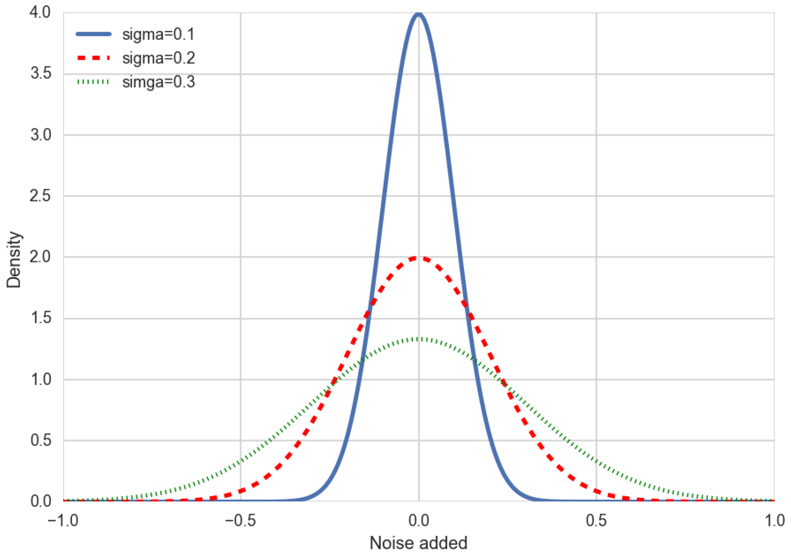
In this work, Gauss distribution is used to include noise in the data. The Gaussian noise is statistical noise with a probability density function equal to that of the Gaussian distribution. Gaussian noise is therefore noise whose frequency spectrum (after a Fourier transform) has a bell-shaped curve.

We compute the Gaussian noise with the following probability density

$$P_G\left(x\right)=\frac{1}{\sqrt{2·\pi ·{\sigma }^2}}·e^{{\displaystyle -\frac{{(x-\mu )}^2}{2·{\sigma }^2}}},$$

(25)

where $\mu$ is the mean and $\sigma$ the standard deviation. We are going to use three amplitudes of noise in the training data. They are computed with the same mean $\mu =0.0$ and different standard deviations’ values (low: $\sigma =0.1$, middle: $\sigma =0.2$ and high: $\sigma =0.3$).

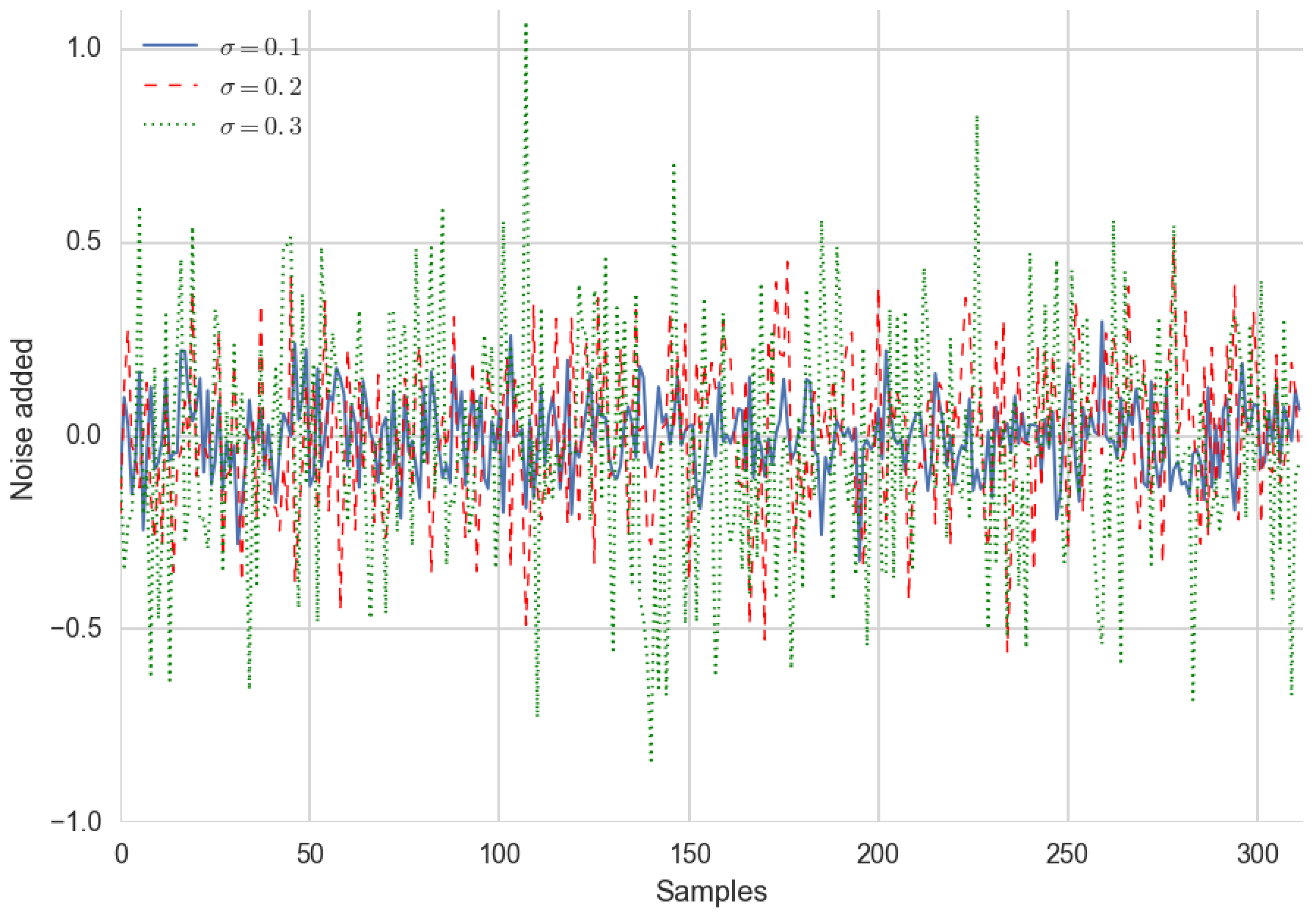
Figure 6 shows the Gaussian probability densities applied for generating Gaussian noise. Figure 7 shows the three Gaussian noises added to training data for each sample.

Regarding this experiment, data gathering in laboratory environments does not include noise, since it is normally clean, the sensors and their connections are very accessible and there is specialised staff in charge of their care. However, in industrial working conditions, the situation changes. In the environment of the sensors, there may be dust, grease and other fouling agents; these sensors are not usually located in points where they can be easily checked and it is not usual to have staff in charge of its continuous review.

In the industrial drying processes in which we are interested, it is usual for distorted data records to invalidate the measurements and therefore the process control should be less accurate. For these reasons, it is worth testing the proposal with noisy data, both Gaussian and uncorrelated uniform.

The results of the peels and seeds experiment with Gaussian noise ($\sigma =0.1$) are detailed in

Table 3. Error measurements | Gaussian $\sigma =0.1$ (Peels and seeds).

	MAE	MSE	MEDAE	${\mathit{R}}^2$
LR	0.14225	0.03307	0.12373	0.82560
k-NN	0.02946	0.00376	0.01350	0.98016
RT	0.03562	0.00288	0.02440	0.98479
RF	0.02972	0.00143	0.02460	0.99245
SVR	0.05008	0.00398	0.04188	0.97899
Sig–ELM	0.00409	6.5164 $\times {10}^{-5}$	0.00189	0.99966
Tanh–ELM	0.00406	6.3064 $\times {10}^{-5}$	0.00208	0.99967
E–ELM	0.00467	4.7990  $\times {\mathbf{10}}^{-\mathbf{5}}$	0.00205	0.99975
SE–ELM	0.00492	5.5861 $\times {10}^{-5}$	0.00244	0.99970

. ELMs achieved better results than the state-of-the-art techniques. Tanh–ELM got the lowest error measurement for MAE, Elliot Symmetric–ELM the lowest scores for MSE and MEDAE and the highest one for $R^2$ score. According to all the error measurements, ELM outperforms the tested forecasting techniques and Elliot–ELM is the best within the ELM flavours. The second-best technique for MAE and MEDAE is k-NN, for MSE and $R^2$ is Random Forest.

The results of the sludge experiment with noise ($\sigma =0.1$) are detailed in

Table 4. Error measurements $\sigma =0.1$ (Sludge).

	MAE	MSE	MEDAE	${\mathit{R}}^2$
LR	0.10773	0.02029	0.08720	0.91963
k-NN	0.02183	0.00084	0.01564	0.99668
RT	0.03704	0.00330	0.02283	0.98692
RF	0.02989	0.00208	0.01958	0.99177
SVR	0.04642	0.00318	0.04004	0.98742
Sig–ELM	0.00367	3.2901 $\times {10}^{-5}$	0.00186	0.99990
Tanh–ELM	0.00264	1.9843 $\times {10}^{-5}$	0.00160	0.99992
E–ELM	0.00244	1.3300 $\times {10}^{-5}$	0.00136	0.99995
SE–ELM	0.00242	1.2976 $\times {\mathbf{10}}^{-\mathbf{5}}$	0.00139	0.99995

. ELMs achieved better results than the state-of-the-art techniques. Elliot–ELM got the lowest error measurement for MAE, MEDAE and the highest one for $R^2$. Elliot Symmetric–ELM got the lowest scores for MSE. According to all the error measurements, ELM outperforms the tested forecasting techniques and Elliot–ELM is the best within the ELM flavours. The second-best technique for MAE, MSE and MEDAE is k-NN, for $R^2$ is Random Forest.

The results of the peels and seeds experiment with noise ($\sigma =0.2$) are detailed in

Table 5. Error measurements $\sigma =0.2$ (Peels and seeds).

	MAE	MSE	MEDAE	${\mathit{R}}^2$
LR	0.14627	0.03447	0.12360	0.81820
k-NN	0.04711	0.00722	0.02079	0.96194
RT	0.03631	0.00296	0.02495	0.98439
RF	0.02998	0.00144	0.02509	0.99238
SVR	0.05245	0.00409	0.04300	0.97841
Sig–ELM	0.01383	0.00040	0.00796	0.99787
Tanh–ELM	0.01329	0.00038	0.00580	0.99797
E–ELM	0.00831	0.00018	0.00404	0.99906
SE–ELM	0.00879	0.00020	0.00449	0.99894

. ELMs achieved better results than the state-of-the-art techniques. Elliot–ELM got the lowest error measurement for all the error measurements. According to all the error measurements, ELM outperforms the tested forecasting techniques and Elliot–ELM is the best within the ELM flavours. The second-best technique for MAE, MSE and $R^2$ is Random Forest and for MEDAE is k-NN.

The results of the sludge experiment with noise ($\sigma =0.2$) are detailed in

Table 6. Error measurements $\sigma =0.2$ (Sludge).

	MAE	MSE	MEDAE	${\mathit{R}}^2$
LR	0.11103	0.02158	0.08537	0.91451
k-NN	0.03367	0.00236	0.02355	0.99065
RT	0.03669	0.00328	0.02157	0.98699
RF	0.02991	0.00209	0.01914	0.99172
SVR	0.04660	0.00314	0.04227	0.98756
Sig–ELM	0.01403	0.00046	0.00739	0.99818
Tanh–ELM	0.01186	0.00032	0.00620	0.99875
E–ELM	0.00734	0.00013	0.00361	0.99947
SE–ELM	0.00747	0.00014	0.00368	0.99945

. ELMs achieved better results than the state-of-the-art techniques. Elliot–ELM got the lowest error measurement for all the error measurements. According to all the error measurements, ELM outperforms the tested forecasting techniques and Elliot–ELM is the best within the ELM flavours. The second-best technique for all the error measurements is Random Forest.

The results of the peels and seeds experiment with noise ($\sigma =0.3$) are detailed in

Table 7. Error measurements with $\sigma =0.3$ (Peels and seeds).

	MAE	MSE	MEDAE	${\mathit{R}}^2$
LR	0.15087	0.03646	0.12148	0.80771
k-NN	0.06856	0.01396	0.03240	0.92637
RT	0.03979	0.00347	0.02518	0.98171
RF	0.03341	0.00206	0.02624	0.98915
SVR	0.05892	0.00516	0.05621	0.97279
Sig–ELM	0.02728	0.00171	0.01659	0.99099
Tanh–ELM	0.02656	0.00158	0.01556	0.99165
E–ELM	0.01924	0.00080	0.00986	0.99580
SE–ELM	0.01869	0.00077	0.01008	0.99594

. ELMs achieved better results than the state-of-the-art techniques. Symmetric Elliot–ELM got the lowest error measurement for MAE, MEDAE and the highest one for $R^2$. Elliot–ELM got the lowest scores for MEDAE. According to all the error measurements, ELM outperforms the tested forecasting techniques and Elliot–ELM is the best within the ELM flavours. The second-best technique for MAE, MSE and MEDAE is k-NN, for $R^2$ is Random Forest.

The results of the sludge experiment with noise ($\sigma =0.3$) are detailed in

Table 8. Error measurements with $\sigma =0.3$ (Sludge).

	MAE	MSE	MEDAE	${\mathit{R}}^2$
LR	0.11543	0.02351	0.08689	0.90689
k-NN	0.04776	0.00465	0.03002	0.98159
RT	0.04407	0.00475	0.02346	0.98119
RF	0.03459	0.00349	0.02008	0.98617
SVR	0.05020	0.00421	0.04268	0.98331
Sig–ELM	0.02692	0.00209	0.01429	0.99173
Tanh–ELM	0.02396	0.00182	0.01249	0.99277
E–ELM	0.02621	0.00177	0.01320	0.99298
SE–ELM	0.02631	0.00186	0.01357	0.99261

. ELMs achieved better results than the state-of-the-art techniques. Elliot–ELM got the lowest error measurement for MSE and the highest one for $R^2$. Tanh–ELM got the lowest scores for MAE and MEDAE. According to all the error measurements, ELM outperforms the tested forecasting techniques and the second-best technique for MAE, MSE and MEDAE and $R^2$ is Random Forest.

7. Conclusions

In this paper, we proposed Elliot and Symmetric Elliot activation functions for Extreme Learning Machine for industrial drying processes’ regression. The authors compare several state-of-the-art techniques and the Elliot-based ELM proposal. Moreover, a range of numbers of neurons in the hidden layer is checked.

The authors applied the proposal to the thermal industry drying process. As far as we know, this is a novel application of Extreme Learning Machines. In addition, in this study, the authors utilise four error measurements for assuring the goodness of the proposal.

According to the results of the experiments, our ELM’s proposal outperforms the state-of-the-art algorithms and Elliot and Symmetric-Elliot ELMs are competitive with the conventional logistic activation functions. Elliot and Symmetric-Elliot ELMs obtained the best performances in most cases.

Furthermore, the experiments were also done with inclusion of three levels of Gaussian noise. Elliot-based ELMs were the best proposals in most of the experiments according to the four error measurements.

References

1. Kavak Akpinar, E.; Bicer, Y.; Cetinkaya, F. Modelling of thin layer drying of parsley leaves in a convective dryer and under open sun. J. Food Eng. 2006, 75, 308–315. [Google Scholar] [CrossRef]
2. Sabarez, H.T.; Price, W.E. A diffusion model for prune dehydration. J. Food Eng. 1999, 42, 167–172. [Google Scholar] [CrossRef]
3. Doymaz, I. Convective air drying characteristics of thin layer carrots. J. Food Eng. 2004, 61, 359–364. [Google Scholar] [CrossRef]
4. Karim, M.D.A.; Hawlader, M.N.A. Drying characteristics of banana: Theoretical modelling and experimental validation. J. Food Eng. 2005, 70, 35–45. [Google Scholar] [CrossRef]
5. Akpinar, E.K. Determination of suitable thin layer drying curve model for some vegetables and fruits. J. Food Eng. 2005, 73, 75–84. [Google Scholar] [CrossRef]
6. Akgun, N.A.; Doymaz, I. Modelling of olive cake thin-layer drying process. J. Food Eng. 2005, 68, 455–461. [Google Scholar] [CrossRef]
7. Doymaz, I. Thin layer drying behaviour of mint leaves. J. Food Eng. 2006, 74, 370–375. [Google Scholar] [CrossRef]
8. Parry, J.L. Mathematical modelling and computer simulation of heat and mass transfer in agricultural grain drying. J. Agric. Eng. Res. 1985, 54, 339–352. [Google Scholar] [CrossRef]
9. Zhang, Y.; Li, Y.; Sun, J.; Ji, J. Estimates on compressed neural networks regression. Neural Netw. 2015, 63, 10–17. [Google Scholar] [CrossRef] [Green Version]
10. Walker, S.H.; Duncan, D.B. Estimation of the probability of an event as a function of several independent variables. Biometrika 1967, 54, 167–178. [Google Scholar] [CrossRef]
11. Altman, N.S. An introduction to kernel and nearest-neighbor nonparametric regression. Am. Stat. 1992, 46, 175–185. [Google Scholar]
12. Papadopoulos, H.; Proedrou, K.; Vovk, V.; Gammerman, A. Inductive confidence machines for regression. In Proceedings of the 2002 European Conference on Machine Learning (ECML), Helsinki, Finland, 19–23 August 2002; pp. 345–356. [Google Scholar]
13. Ho, T.K. The Random Subspace Method for Constructing Decision Forests. IEEE Trans. Pattern Anal. Mach. Intell. 1998, 20, 832–844. [Google Scholar]
14. Drucker, H.; Burges, C.J.C.; Kaufman, L.; Smola, A.J.; Vapnik, V.N. Support Vector Regression Machines. Adv. Neural Inf. Process. Syst. (NIPS) 1997, 9, 155–161. [Google Scholar]
15. Toğrul, I.; Pehlivan, D. Mathematical modelling of solar drying of apricots in thin layers. J. Food Eng. 2002, 55, 209–216. [Google Scholar] [CrossRef]
16. Karim, M.; Perez, E.; Amin, Z.M. Mathematical modelling of counter flow v-grove solar air collector. Renew. Energy 2014, 67, 192–201. [Google Scholar] [CrossRef]
17. Notton, G.; Motte, F.; Cristofari, C.; Canaletti, J.L. New patented solar thermal concept for high building integration: Test and modeling. Energy Procedia 2013, 42, 43–52. [Google Scholar] [CrossRef]
18. Dowson, M.; Pegg, I.; Harrison, D.; Dehouche, Z. Predicted and in situ performance of a solar air collector incorporating a translucent granular aerogel cover. Energy Build. 2012, 49, 173–187. [Google Scholar] [CrossRef] [Green Version]
19. Huang, G.; Ding, X.; Zhou, H. Optimization method based extreme learning machine for classification. Neurocomputing 2010, 74, 155–163. [Google Scholar] [CrossRef]
20. De, G.; Gao, W. Forecasting China’s Natural Gas Consumption Based on AdaBoost-Particle Swarm Optimization-Extreme Learning Machine Integrated Learning Method. Energies 2018, 11, 2938. [Google Scholar] [CrossRef]
21. Madhusudhanan, S.; Jaganathan, S.; Jayashree, L. Incremental Learning for Classification of Unstructured Data Using Extreme Learning Machine. Algorithms 2018, 11, 158. [Google Scholar] [CrossRef]
22. Salerno, V.M.; Rabbeni, G. An Extreme Learning Machine Approach to Effective Energy Disaggregation. Electronics 2018, 7, 235. [Google Scholar] [CrossRef]
23. Huang, G.B.; Zhu, Q.Y.; Siew, C.K. Extreme Learning Machine: Theory and Applications. Neurocomputing 2006, 70, 489–501. [Google Scholar] [CrossRef]
24. Nobrega, J.P.; Oliveira, A.L. Kalman filter-based method for Online Sequential Extreme Learning Machine for regression problems. Eng. Appl. Artif. Intell. 2016, 44, 101–110. [Google Scholar] [CrossRef]
25. Zhang, Y.; Wu, J.; Cai, Z.; Zhang, P.; Chen, L. Memetic Extreme Learning Machine. Pattern Recognit. 2016, 58, 135–148. [Google Scholar] [CrossRef]
26. Zhao, X.; Bi, X.; Wang, G.; Wang, C.; Yang, H. Uncertain xml documents classification using extreme learning machine. Neurocomputing 2016, 174, 375–382. [Google Scholar] [CrossRef]
27. Rao, C.; Mitra, S. Generalized Inverse of Matrices and its Applications; Wiley: New York, NY, USA, 1971. [Google Scholar]
28. Shamshirban, S.; Mohammadi, K.; Tong, C.W.; Petković, D.; Porcu, E.; Mostafaeipour, A.; Ch, S.; Sedaghat, A. Application of extreme learning machine for estimation of wind speed distribution. Clim. Dyn. 2016, 46, 1893–1907. [Google Scholar] [CrossRef]
29. Elliott, D.L. A Better Activation Function for Artificial Neural Networks; Technical Research Report; Institute for Systems Research: College Park, MD, USA, 1993. [Google Scholar]
30. Sibi, P.; Allwynjones, S.; Siddarth, P. Analysis of different activation functions using backpropagation neural networks. J. Theor. Appl. Inf. Technol. 2013, 47, 1264–1268. [Google Scholar]
31. Mendil, B.; Benmahammed, K. Simple activation functions for neural and fuzzy neural networks. In Proceedings of the IEEE International Symposium on Circuits and Systems, Orlando, FL, USA, 30 May–2 June 1999; pp. 347–350. [Google Scholar]
32. Ruiz-Celma, A.; Cuadros, F.; Lopez-Rodríguez, F. Convective drying characteristics of sludge from treatment plants in tomato processing industries. Food Bioprod. Process. 2012, 90, 224–234. [Google Scholar] [CrossRef]
33. Ruiz-Celma, A.; Cuadros, F.; Lopez-Rodriguez, F. Thin layer drying behavior of industrial tomato by-products in a convective dryer at low temperatures. Res. J. Biotechnol. 2013, 8, 50–60. [Google Scholar]
34. Yan, X. Linear Regression Analysis: Theory and Computing; World Scientific: Singapore, 2009. [Google Scholar]
35. Cover, T. Estimation by the nearest neighbor rule. IEEE Trans. Inf. Theory 1968, 14, 50–55. [Google Scholar] [CrossRef] [Green Version]
36. Kenesei, T.; Abonyi, J. Hinging hyperplane based regression tree identified by fuzzy clustering and its application. Appl. Soft Comput. 2013, 13, 782–792. [Google Scholar] [CrossRef]
37. Ortuno, F.M.; Valenzuela, O.; Prieto, B.; Saez-Lara, M.J.; Torres, C.; Pomares, H.; Rojas, I. Comparing different machine learning and mathematical regression models to evaluate multiple sequence alignments. Neurocomputing 2015, 164, 123–136. [Google Scholar] [CrossRef]
38. Czajkowski, M.; Kretowski, M. The role of decision tree representation in regression problems—An evolutionary perspective. Appl. Soft Comput. 2016, 48, 458–475. [Google Scholar] [CrossRef]
39. Breiman, L. Random forests. Mach. Learn. 2001, 45, 5–32. [Google Scholar] [CrossRef]
40. Vapnik, V. The Nature of Statistical Learning Theory; Springer: New York, NY, USA, 1995. [Google Scholar]
41. Smola, A.; Schölkopf, B. A tutorial on support vector regression. Stat. Comput. 2004, 14, 199–222. [Google Scholar] [CrossRef] [Green Version]
42. Schölkopf, B.; Smola, A. Learning with Kernels-Support Vector Machines, Regularisation, Optimization and Beyond; The MIT Press: Cambridge, MA, USA, 2001. [Google Scholar]
43. ISO 32001:1981. Hard Coal and Anthracite. Determination of Total Moisture; ISO: Geneva, Switzerland, 1981. [Google Scholar]
44. Wang, R.Y.; Storey, V.C.; Firth, C.P. A framework for analysis of data quality research. IEEE Trans. Knowl. Data Eng. 1995, 7, 623–640. [Google Scholar] [CrossRef] [Green Version]
45. Zhu, X.; Wu, X. Class Noise vs. Attribute Noise: A Quantitative Study. Artif. Intell. Rev. 2004, 22, 177–210. [Google Scholar] [CrossRef]
Figure 1. Extreme learning machine.
Energies 12 00090 g001
Figure 2. Hidden layer neurons.
Energies 12 00090 g002
Figure 3. Activation functions.
Energies 12 00090 g003
Figure 4. Experimental setup.
Energies 12 00090 g004
Figure 5. ELM-based drying model.
Energies 12 00090 g005
Figure 6. Gaussian noise probability densities.
Energies 12 00090 g006
Figure 7. Gaussian noise waveform.
Energies 12 00090 g007