Wind Speed Modeling by Nested ARIMA Processes

Abstract

Wind speed modelling is of increasing interest, both for basic research and for applications, as, e.g., for wind turbine development and strategies to construct large wind power plants. Generally, such modelling is hampered by the non-stationary features of wind speed data that, to a large extent, reflect the turbulent dynamics in the atmosphere. We study how these features can be captured by nested ARIMA models. In this approach, wind speed fluctuations in given time windows are modelled by one stochastic process, and the parameter variation between successive windows by another one. For deriving the wind speed model, we use 20 months of data collected at the FINO1 platform at the North Sea and use a variable transformation that best maps the wind speed onto a Gaussian random variable. We find that wind speed increments can be well reproduced for up to four standard deviations. The distributions of extreme variations, however, strongly deviate from the model predictions.

1. Introduction

When planning wind power plants, the choice of its location as well as the precise positions of the composing wind turbines depend on estimates of wind speed at those particular spots. By deriving efficient models that can, under certain accuracy, convert wind speed estimates into wind power estimates, one is able to forecast deficit and excess of generated power and decide in advance the amount of necessary energy to handle in the market and for maintaining stable functioning of power grids.

ARIMA (Autoregressive Integrated Moving Average) models have been often used in the last decades [1] for modelling wind speed and wind power variations over large time lags, typically of the order of one hour. They are simple to implement and, if of low order, can be interpreted as discretised forms of differential equations. They were used for modelling output of wind power plants in connection with investment strategies in the energy market [2], variations of energy demand [3], and monthly variations of wind power generation [4]. For describing fluctuations, on shorter time-scales of about 10 min, ARIMA models could be applied by increasing the number of regression and moving average terms (higher order) and introducing frequency decomposition [5]. One main advantage of ARIMA models is their cheap computational cost, since they are based on simple iterative procedures [6].

More sophisticated recursive models are the so-called artificial neural networks, which include nonlinear terms and derive the weight of each particular contribution through a learning process, based on previous sets of measurements. They have been applied also for wind speed prediction [7]. Though more precise in value prediction than standard ARIMA models [8,9], artificial neural networks are difficult to interpret due to their higher complexity.

For this reason, ARIMA models remain as a widely used approach for wind speed modelling [10], sometimes in combination with other methods. For example, hourly and ten minute averages of wind speed data collected in Mexico were modelled with an ARIMA model and compared with a neural network that uses additional exogenous meteorological variables [8]. Though using considerably more data, neural networks seem to guarantee improvements not better than 6%. ARIMA models with exogenous variables have been also developed [11] for modelling 15 min average wind speed. By studying wind speed series from China, it has been found that an ARIMA model combined with empirical mode decomposition has a better accuracy in comparison with neural networks and other machine learning approaches [12], achieving a mean absolute error smaller than 4%. However, this accurary is obtained for ten minute averages. For one hour, the accuracy of all models decreases considerably. A further approach, using empirical mode decomposition in combination with neural networks, was followed in [13]. In a recent review, different approaches for modelling ultra-short, short, medium and long-term wind speed fluctuations are discussed [14], including neural networks, ARIMA models and wavelet methods.

With respect to wind data analysis, there are two major issues that challenge the application and usefulness of ARIMA models. First, wind speeds are not Gaussian distributed, but typically can be well described by a Weibull distribution [15]. Secondly, the distribution of wind speed increments is also not Gaussian, showing fat tails [16]. These issues raise the question whether these problems can be resolved by a refined approach based on ARIMA processes. In this paper, we investigate up to which extent ARIMA models can reproduce statistical features of wind speed data, by addressing both these issues. We focus on 15 min of wind speed measurements collected at the FINO1 platform at the North Sea [17], see Figure 1a,b. These measurements were performed over a period of 20 months with a sample frequency of 1 Hz. The choice of 15 min is motivated by forecasting strategies in energy markets, which commonly use predictions of energy production 15 min ahead.

To address the non-Gaussianity of wind speed distributions, we consider a transformed variable, which is a power of the wind speed. The respective exponent is determined by the requirement that the distribution of the transformed variable fits a Gaussian distribution as best as possible. The corresponding optimisation procedure is outlined in the Appendix A, where we provide a table also of exponent values as a function of the two parameters specifying the Weibull distribution. This can be used for other wind speed data sets.

We find that the best ARIMA model for the wind speed data on the time scale of 15 min is an ARIMA$(0,1,2)$ model. The coefficients change for each 15 min window and are also modelled by ARIMA processes. We call this combination of the ARIMA$(0,1,2)$ model with the ARIMA models for its coefficients a nested ARIMA model and show that it is able to predict distributions of wind speed increments over a range of up to four standard deviations. Beyond this range, however, this approach has its limits. The methodology resembles that of the so-called superstatistics approach [18] and earlier work on the distribution of velocity increments in turbulent flows [19]. Distribution parameters have been modelled with stochastic differential equations, for instance to model the evolution of volume-price distributions in the stock exchange [20,21]. Stochastic differential equations are a further means of data modelling and can in general be interpreted straightforwardly. They have been recently applied for describing short-time fluctuations of wind power outputs in wind turbines and wind farms [22,23].

In Section 2, we describe the ARIMA model for the wind speed and its parameters. In Section 3, we first describe the data used and the pre-processing of these data. Then, we derive the ARIMA model that best suits the set of measurements on the scale of 15 min. In Section 4, we introduce the nested ARIMA model and compare its predictions for the distributions of wind speed increments with the corresponding distributions of the measured values. In Section 5, we summarise our main results and discuss their implications for future research.

2. ARIMA-Model

ARIMA model stands for Autoregressive Integrated Moving Average model [10], where the evolution of a variable x in discrete time t is described as

$${\Delta }^d{x}_t=\sum _{j=1}^p{\varphi }_j{\Delta }^d{x}_{t-j}+\sum _{k=1}^q{\theta }_k{w}_{t-k}+w_t.$$

(1)

Here, p, d and q are the parameters quantifying the order of the model, usually represented as $(p,d,q)$, ${\varphi }_j$ ($j=1,\cdots ,p$) and ${\theta }_k$ ($k=1,\cdots ,q$) are coefficients, and $w_k$ are uncorrelated Gaussian random numbers with zero mean and variance ${\sigma }_w^2$. The operator $\Delta$ corresponds to a discrete derivative and is defined as

$$\Delta x_t=x_t-x_{t-1}.$$

(2)

Without loss of generality, the mean of $x_t$ is zero. Parameter d specifies the minimum number of “differentiations” needed to map the original (possibly non-stationary) process onto a stationary process. Parameter p specifies the number of previous x values entering the ARIMA process and defines the order of the auto-regressive (AR) part of the model. Parameter q gives the number of previous additive Gaussian white noise terms and defines the order of the moving average (MA) part of the model.

For modelling a time series ${\left\{x_t\right\}}_{1\le t\le N}$, an ARIMA process can be derived by estimating its order $(p,d,q)$, the sets $\varphi ={\left\{{\varphi }_j\right\}}_{1\le j\le p}$, $\theta ={\left\{{\theta }_k\right\}}_{1\le k\le q}$ of coefficients and the noise strength ${\sigma }_w$ by a maximum likelihood estimator in combination with the Bayesian Information Criterion [24]. The corresponding procedure is illustrated in Figure 2 for a test series ${\left\{x_t^{\left(\mathrm{test}\right)}\right\}}_{1\le t\le N}$ of $N={10}^5$ values generated by Equation (1) with $(p,d,q)=(2,1,2)$, ${\sigma }_w=0.1$, and coefficients ${\varphi }_1=0.5$, ${\varphi }_2=-0.1$, ${\theta }_1=0.3$, and ${\theta }_2=-0.2$. The test series is shown in Figure 2a, and in Figure 2b the series of its increments $\Delta x_t^{\left(\mathrm{test}\right)}=[x_t^{\left(\mathrm{test}\right)}-x_{t-1}^{\left(\mathrm{test}\right)}]$ is plotted; the corresponding distributions are shown in the right panels of these graphs.

To estimate parameter d, the unit-root test [10] is performed, starting with $d=0$. In case it fails, the order d is increased by one and the test repeated. The first value of d for which ${\Delta }^d{x}_t$ fulfils the unit-root test is chosen. For the series ${\left\{x_t^{\left(\mathrm{test}\right)}\right\}}_{1\le t\le N}$, this yielded the correct value $d=1$.

To determine q and p, first maximal values ${\tau }_q$ and ${\tau }_p$ of these parameters are estimated from analysing the autocorrelation function (ACF) and the partial autocorrelation function (PACF) of the time series ${\left\{x_t\right\}}_{1\le t\le N}$, respectively [10,25]. The ACF measures the correlation between two increment values ${\Delta }^d{x}_t$ and ${\Delta }^d{x}_{t+\tau }$ and, for $d=1$; it is given by

$$\gamma \left(\tau \right)=\frac{\langle \Delta x_{t+\tau }\Delta x_t\rangle }{{\sigma }^2},$$

(3)

where ${\sigma }^2$ is the variance of the increments $\Delta x_t$. In general, the ACF must be defined with time-dependent variances ${\sigma }_x^2\left(t\right),{\sigma }_x^2(t+\tau )$, but in this case the time series $\Delta x_t$ is stationary and ${\sigma }^2$ becomes time-independent. For the test series, the ACF is shown in Figure 2c. The upper bound ${\tau }_q$ of q is estimated from the smallest value of $\tau$, where the ACF becomes negative, i.e., ${\tau }_q={min}_{\tau }\{\gamma \left(\tau \right)<0\}$. In Figure 2c, the corresponding value ${\tau }_q=3$ is indicated by the arrow.

The PACF quantifies the direct correlation between $x_t$ and $x_{t-\tau }$ after removing the linear dependence on the intermediate values $x_{t-k}$ with $k=1,\cdots ,\tau -1$. Specifically, the PACF $\phi \left(\tau \right)$ is the last component of the vector [25]

$$\begin{array}{ccc}\hfill \left(\begin{array}{c}\phi \left(1\right)\\ ⋮\\ ⋮\\ \phi \left(\tau \right)\end{array}\right)& =& {\left(\begin{array}{cccc}\gamma \left(0\right)& \gamma \left(1\right)& \cdots & \gamma (\tau -1)\\ \gamma \left(1\right)& \gamma \left(0\right)& \cdots & \gamma (\tau -2)\\ ⋮& ⋮& ⋮& ⋮\\ \gamma (\tau -1)& \gamma (\tau -2)& \cdots & \gamma \left(0\right)\end{array}\right)}^{-1}\left(\begin{array}{c}\gamma \left(1\right)\\ ⋮\\ ⋮\\ \gamma \left(\tau \right)\end{array}\right).\hfill \end{array}$$

(4)

For the test series, the PACF is shown in Figure 2d. We estimate the upper bound ${\tau }_p$ from a least square fit of $\left|\phi \right(\tau \left)\right|$ to an exponential decay $\left|\phi \left(0\right)\right|exp(-\tau /{\tilde{\tau }}_p)$, where ${\tau }_p=\mathrm{int}\left({\tilde{\tau }}_p\right)+1$. The corresponding value ${\tau }_p=4$ is indicated by the arrow in Figure 2d.

Given d as well as p and q in $0\le p\le {\tau }_p$ and $0\le p\le {\tau }_q$, a maximum likelihood function estimator can be defined, based on assumptions regarding Gaussian statistics of residuals and by using reasonable initialisations of the recurrence Equation (1) (see, e.g., reference [10] for details). The likelihood function ${\mathcal{L}}_X(\varphi ,\theta ,{\sigma }_w)$ estimates the probability of finding the time series $X={\left\{x_t\right\}}_{1\le t\le N}$ realised for the sets $\varphi ={\left\{{\varphi }_j\right\}}_{1\le j\le p}$, $\theta ={\left\{{\theta }_k\right\}}_{1\le k\le q}$ of coefficients and the noise strength ${\sigma }_w$ in the ARIMA process (1). Maximising ${\mathcal{L}}_X(\varphi ,\theta ,{\sigma }_w)$ with respect to the model parameters, best estimators $\widehat{\varphi }(p,q)$, $\widehat{\theta }(p,q)$, and ${\widehat{\sigma }}_w(p,q)$ are obtained for each p and q.

The maximum likelihood method yields parameter sets for each p and q, but one still needs to decide which of the p and q in the ranges $0\le p\le {\tau }_p$ and $0\le p\le {\tau }_q$ should be selected. Larger p and q will give better maximised likelihoods, but at the price of a higher complexity of the model. To take into account both (i) how well the models fit the data, quantified by the likelihood $\mathcal{L}(\widehat{\varphi }(p,q),\widehat{\theta }(p,q),{\widehat{\sigma }}_w(p,q))$, and (ii) how many parameters are needed for obtaining this likelihood, the Bayesian Information Criterion (BIC) [24]

$${\mathcal{B}}_X(p,q)=(p+q+1)lnN-2ln{\mathcal{L}}_X(\widehat{\varphi }(p,q),\widehat{\theta }(p,q),{\widehat{\sigma }}_w(p,q))$$

(5)

is often introduced. The best values p and q are the ones yielding the smallest ${\mathcal{B}}_X(p,q)$. For the test series ${\left\{x_t^{\left(\mathrm{test}\right)}\right\}}_{1\le t\le N}$, we obtain the correct order $(p,d,q)=(2,1,2)$ and coefficients values that, within the numerical uncertainties, agree with the values used for generating the series: ${\widehat{\varphi }}_1=0.49\pm 0.03$, ${\widehat{\varphi }}_2=-0.101\pm 0.005$, ${\widehat{\theta }}_1=0.31\pm 0.03$, ${\widehat{\theta }}_2=-0.20\pm 0.02$, and ${\widehat{\sigma }}_w^2=0.01$. The error associated to the variance of the Gaussian noise can be estimated as $SE\left({\widehat{\sigma }}_w^2\right)={\widehat{\sigma }}_w^2\sqrt{2/(N-1)}\sim 4\times {10}^{-5}$.

With this estimation of the parameters, it is clear that the respective adapted ARIMA$(2,1,2)$ model with $\widehat{\varphi }$, $\widehat{\theta }$ and ${\widehat{\sigma }}_w$ would give predictions within an uncertainty that almost agrees with the intrinsic noise of the ARIMA$(2,1,2)$ process used for generating the test series. It is instructive to compare corresponding predictions with the simplest prediction model, the maximum persistence model with ${\widehat{x}}_{t+1}=x_t$. In Figure 2e, we show, as an example, 30 predicted data values of the adapted ARIMA$(2,1,2)$ process and that of the maximum persistence model in comparison with additional data ($N={10}^5+k$, $k=1,2,\dots$) generated for the test series. In the right panel of this figure, the distributions of the deviations between predicted and generated data are shown. The smaller width of the distribution for the adapted ARIMA model shows that it significantly improves the prediction quality over the maximum persistence model.

To evaluate the accuracy of the method described above for determining p and q, we generated a number n of test series ${\left\{x_t^{\left(j\right)}\right\}}_{1\le t\le N}$, $j=1,\dots ,n$, for the same ARIMA(2, 1, 2) model and determined the fraction of series, where the above analysis recovers the correct values. The so estimated accuracy will increase with the size N of the test series. This is shown in Figure 2f, where the accuracy, estimated from $n=250$ test series, is plotted as a function of N for the case $(p,d,q)=(2,1,2)$. It can be seen that for $N\gtrsim {10}^3$, the accuracy becomes larger than 90%.

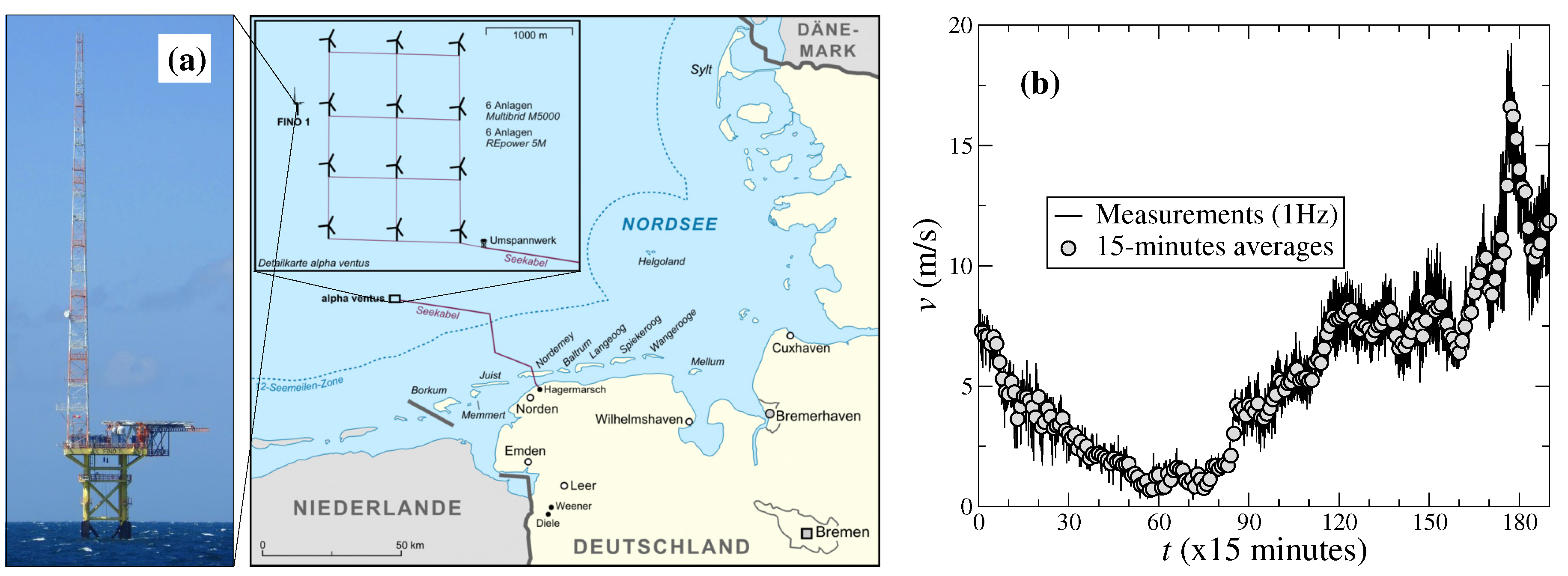
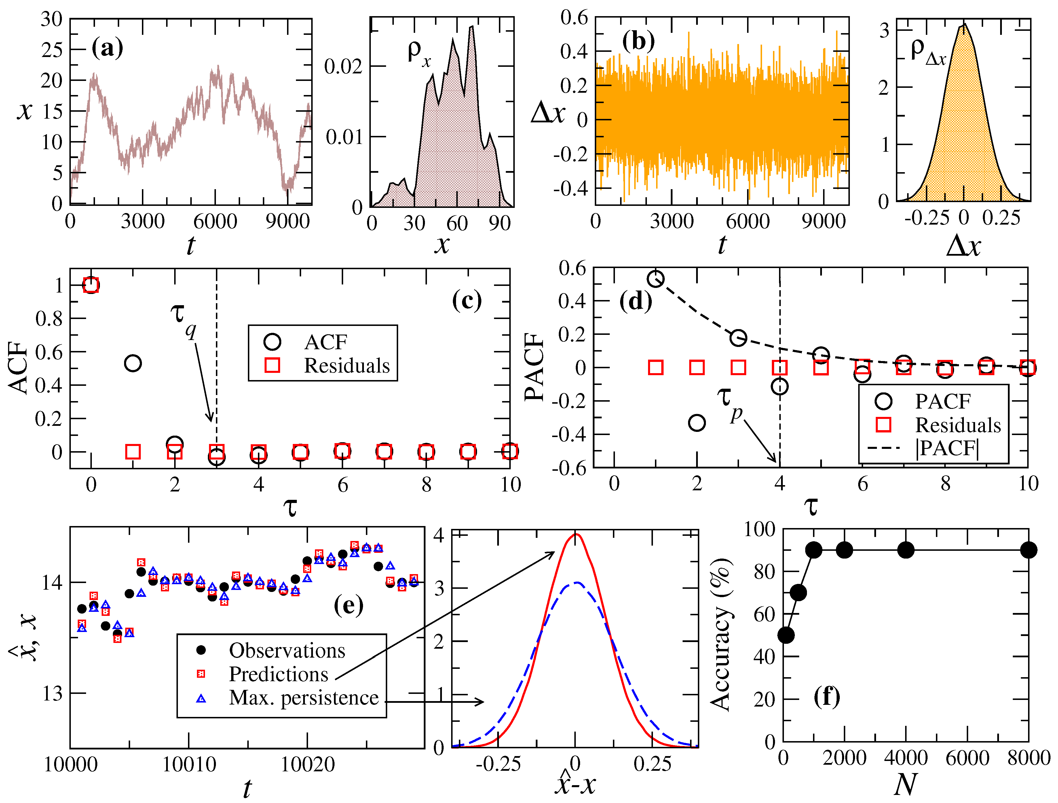
3. ARIMA Model for Wind Speed Measurements

We analyse data collected at the FINO1 platform, which is located about 45 km north from the island of Borkum in the North Sea (see Figure 1a). The wind speeds were measured over 20 months, from September 2015 to April 2017, at a sampling frequency of $1\mathrm{Hz}$. The FINO1 platform measures wind speed at eight different heights. Here, we consider the measurements at a height of 100 m, taken by a cup anemometer.

As illustrated in Figure 1b, the series ${\left\{v\left(m\right)\right\}}_{1\le m\le M}$ of 20 months wind speed data ($M\cong 5.2\times {10}^7$) is transformed into a series of backward averages over $M_0=900$ values, corresponding to 15 min,

$$\overline{v}\left(t\right)=\frac{1}{M_0}\sum _{t^{\prime }=M_0(t-1)+1}^{t{M}_0}v\left(t^{\prime }\right),t=1,2,\dots ,N\cong 5.8\times {10}^4.$$

(6)

This series of backward-averaged values is shown in Figure 3a. All windows of 15 min data having more than 25% missing data (225 values) were disregarded. In total, this pre-processing resulted in only 65 missing $\overline{v}$ values. The distribution of the $\overline{v}$, shown in Figure 3b, is well fitted by a Weibull form

$${\rho }_{\mathrm{W}}\left(\overline{v}\right)=\frac{k}{\lambda }{\left(\frac{\overline{v}}{\lambda }\right)}^{k-1}exp\left[-{(\overline{v}/\lambda )}^k\right],$$

(7)

with scale parameter $\lambda$ and shape parameter k. By least square fitting, we obtained $\lambda =10.17$ m/s and $k=2.07$, corresponding to a mean ${\mu }_{\overline{v}}=9.16$ m/s and standard deviation ${\sigma }_{\overline{v}}=4.76$ m/s.

Because ARIMA models yield Gaussian distributed values, we consider a transformed variable u, which is a power law of the wind speed, i.e.,

$$u={\overline{v}}^{\alpha }$$

(8)

with $0<\alpha <1$. An optimal value ${\alpha }_{\mathrm{opt}}$ of $\alpha$ is determined by requiring the distribution of values in the series ${\left\{u\left(t\right)\right\}}_{1\le t\le N}={\left\{{\left[\overline{v}\left(t\right)\right]}^{\alpha }\right\}}_{1\le t\le N}$ to be close to a Gaussian. The corresponding optimisation procedure is described in the Appendix A and yields ${\alpha }_{\mathrm{opt}}=0.586\pm {10}^{-3}$ for the series ${\left\{\overline{v}\left(t\right)\right\}}_{1\le t\le N}$. Figure 3c shows ${\left\{u\left(t\right)\right\}}_{1\le t\le N}$ and in Figure 3d the respective distribution of u values is plotted (symbols). The mean and standard deviation of this distribution are ${\mu }_u=3.53$ (m/s)${}^{{\alpha }_{\mathrm{opt}}}$ and ${\sigma }_u=1.14$ (m/s)${}^{{\alpha }_{\mathrm{opt}}}$. As can be seen from Figure 3d, the Gaussian distribution (dashed lines) with ${\mu }_u$ and ${\sigma }_u$ fits the data (symbols) well.

Previous works have considered other values of $\alpha$, e.g., $\alpha =1/2$ in Ref. [1] and $\alpha =1/3$ in Ref. [26]. In general, the optimal exponent varies from one data sample to another. The optimisation procedure in the Appendix A gives ${\alpha }_{\mathrm{opt}}$ in dependence of the Weibull parameters $\lambda$ and k, and we provide a table of ${\alpha }_{\mathrm{opt}}$ values for k and $\lambda$ lying in ranges typical for wind speed distributions.

We now intend to adapt an ARIMA model to the transformed wind speed u. To this end, we consider time windows shorter than the full 20-month series for the following reasons: firstly, we want to validate whether there exists a typical order $(p,d,q)$ of the ARIMA model. Secondly, for practical applications, one cannot expect data to be available over a period as large as 20 months. As illustrated above, cf. Figure 2f, about 1000 values are sufficient to estimate the parameters of the ARIMA model with good accuracy. We fix the size of the time window to $N_s=3\times {10}^3$ (approximately one month). This yields a total of $n_s\simeq 5.5\times {10}^4$ training series ${\left\{u(t^{\prime }+t)\right\}}_{1\le t\le N_s}$, $t^{\prime }=1,\dots ,n_s$. In case a training series contains some of the 65 missing $\overline{v}$-values (see above), we consider a slightly smaller $N_s$.

We now apply the methods described in the previous Section 2 to obtain ARIMA models for each of the training series. In all cases, we find $d=1$. The analysis of the ACF and PACF was performed for the complete series ${\left\{u\left(t\right)\right\}}_{1\le t\le N}$ and yielded ${\tau }_p={\tau }_q=5$. The p and q values for the training series vary and their joint histogram is shown in Figure 4. In this histogram, a maximum occurs at $(p,q)=(0,2)$. We therefore consider $(p,d,q)=(0,1,2)$ as the order of the ARIMA model for predicting 15 min wind speed averages in our data set.

Next, we evaluate the power of the ARIMA$(0,1,2)$ model to predict values $\widehat{u}\left(t\right)$ for $u\left(t\right)$ from the series ${\left\{u\left(t^{\prime }\right)\right\}}_{t-N_s\le t^{\prime }\le t-1}$ of $N_s=3\times {10}^3$ previous values. The previous values are used to determine the optimal model parameters ${\widehat{\theta }}_1$, ${\widehat{\theta }}_2$ and ${\widehat{\sigma }}_w$ with the maximum likelihood estimator, and the ARIMA process with these optimal parameters gives the respective model series ${\left\{\widehat{u}\left(t^{\prime }\right)\right\}}_{t-N_s\le t^{\prime }\le t-1}$. The prediction is obtained by setting $w_t=\langle w_t\rangle =0$ in Equation (1), and by replacing $w_{t-1}$ and $w_{t-2}$ with the residuals ${ϵ}_{t-1}$ and ${ϵ}_{t-2}$,

$$\widehat{u}\left(t\right)=u(t-1)+{\theta }_1{ϵ}_{t-1}+{\theta }_2{ϵ}_{t-2}=u(t-1)+{\theta }_1[u(t-1)-\widehat{u}(t-1)]+{\theta }_2[u(t-2)-\widehat{u}(t-2)].$$

(9)

The corresponding prediction for the 15 min averaged wind speed is $\widehat{\overline{v}}\left(t\right)=\widehat{u}{\left(t\right)}^{1/{\alpha }_{\mathrm{opt}}}$.

Figure 5a shows the first 30 predictions $\widehat{\overline{v}}\left(t\right)$ (open circles), $t=3001,\cdots ,3030$, in comparison with the measured values $\overline{v}\left(t\right)$ (full circles). Compared to the simple maximum persistence prediction, ${\widehat{\overline{v}}}_{\mathrm{pers}}(t+1)=\overline{v}\left(t\right)$ (crosses), it does not give a significant improvement. This can be clearly seen from Figure 5b, where the distribution of the deviations between each of the models and the real measurement is shown. We find in both cases an average of zero $(\langle {\widehat{\overline{v}}}_{\mathrm{model}}-\overline{v}\rangle \simeq 3\times {10}^{-3})$ and similar standard deviations, ${\sigma }_{\left(012\right)}=0.7495$ and ${\sigma }_{\mathrm{pers}}=0.7525$.

One could suppose that the predictive power of the ARIMA modelling becomes better, when taking higher orders $(p,q)$ (with $d=1$ kept fixed). However, when performing an analysis with such models of higher order, we obtained results comparable to those shown in Figure 5.

To evaluate the performance of the ARIMA model, we consider the mean absolute percentual error (MAPE) defined as

$$\mathrm{MAPE}=\frac{1}{n}\sum _{i=1}^n\left|\frac{{\widehat{v}}_i-v_i}{\overline{v}}\right|$$

(10)

of the wind speed increments. Here, ${\widehat{v}}_i$ denotes the prediction of the ith measured value of the wind speeds, and $v_i$ is the corresponding measured value. The mean of wind speeds is denoted by $\overline{v}$.

Table 1. Performance of the ARIMA(0,1,2) model, using the metric defined in Equation (10), in comparison with different data sets and models reported in [14].

Model	MAPE
ARIMA$(0,1,2)$ (Speed, 15 min.)	5.53%
ARIMA (Speed, 10 min.)	17.61%
ARIMA (Speed, 20 min.)	20.59%
Neural Network (Speed, 10 min.)	5.97%
Neural Network (Speed, 20 min.)	7.03%
ARIMA with Neural Net. (Speed, 10 min.)	4.46%
ARIMA with Neural Net. (Speed, 20 min.)	5.31%

shows the results of our ARIMA$(0,1,2)$ model together with the values obtained for other models. The MAPE of the ARIMA$(0,1,2)$ process shows values comparable to the most accurate ARIMA models.

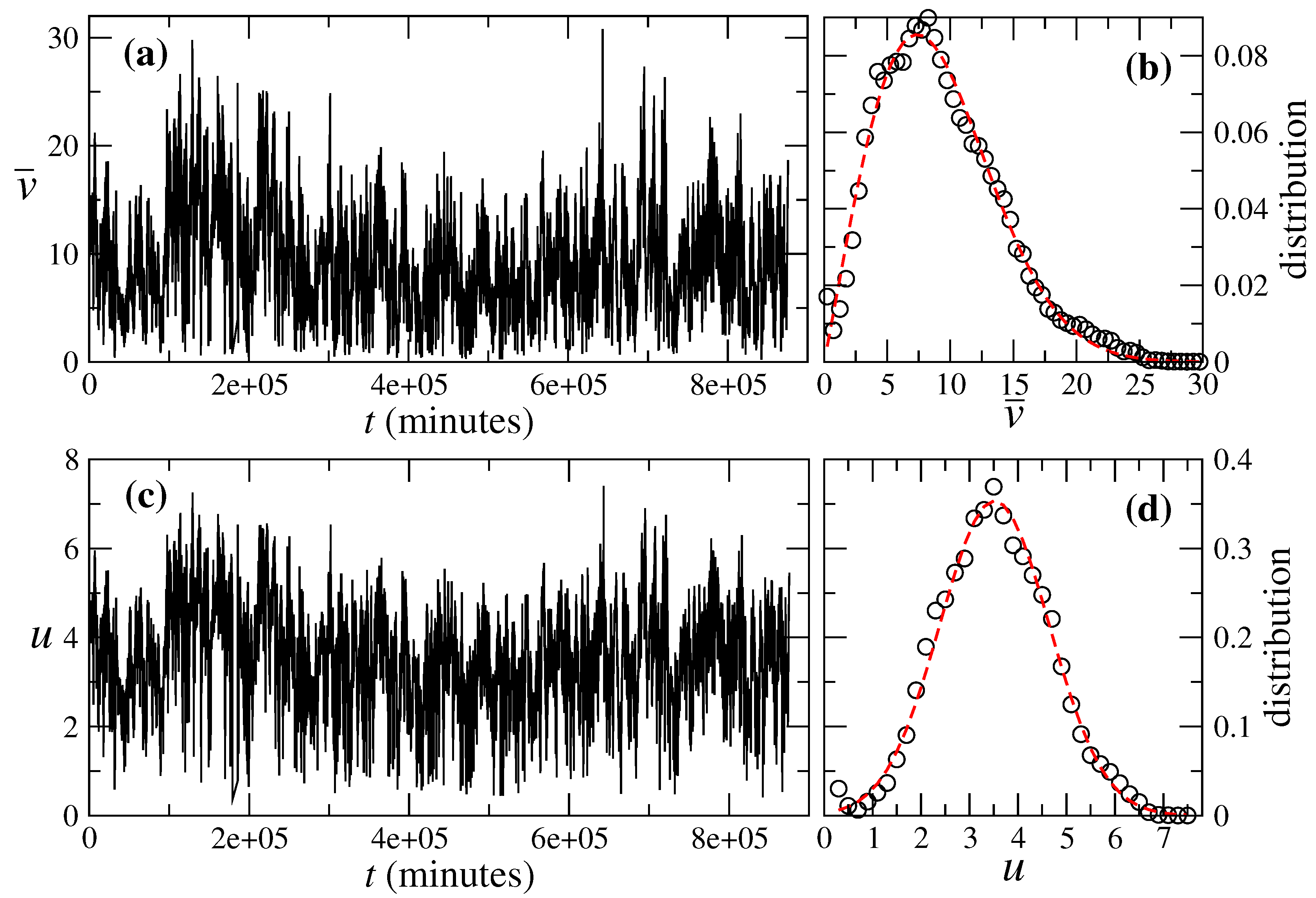
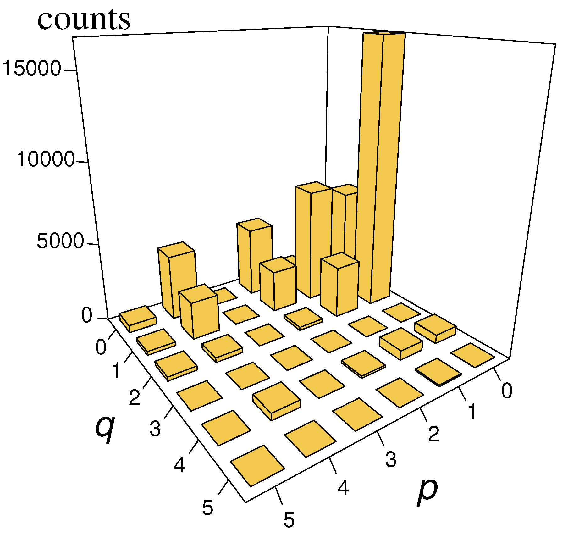
4. Nested ARIMA Model for Wind Speeds

Apart from the prediction of wind speeds based on previous values, it is an important issue to develop tools for generating surrogate wind speed data with statistical features that resemble key features of real data. This allows researchers to use such surrogate data in studies without access to real data, or when an averaging over a large amount of data is required. As mentioned in the Introduction, the distribution of wind speed increments $[\overline{v}(t+\tau )-\overline{v}\left(t\right)]$ for a time lag $\tau$ shows also strong deviations from a Gaussian. As the ARIMA$(0,1,2)$ with fixed parameters ${\theta }_1$, ${\theta }_2$, and ${\sigma }_w$ corresponds to a simple random walk, it is clear that the time variation of these parameters is important for obtaining non-Gaussian features for the increments. In the prediction procedure described in Section 3, the time variations is mediated by the optimal adaptation of the model parameters to the set of $N_s=3\times {10}^3$ previous, and assumed to be known real values.

For generating surrogate data, we now consider the corresponding time series of optimal parameters ${\widehat{\theta }}_1\left(t\right)$, ${\widehat{\theta }}_2\left(t\right)$, and ${\widehat{\sigma }}_w\left(t\right)$. For convenient notation, we will write ${\theta }_1\left(t\right)$, ${\theta }_2\left(t\right)$, and ${\sigma }_w\left(t\right)$ for these series, i.e., we drop the circumflex. As for ${\sigma }_w\left(t\right)$, we consider its (normalised) logarithm,

$$\zeta \left(t\right)=log\left(\frac{{\sigma }_w\left(t\right)}{{\overline{\sigma }}_w}\right),$$

(11)

where ${\overline{\sigma }}_w$ represent the average over all ${\sigma }_w\left(t\right)$. The use of the logarithm is motivated by a previous study [19], where the distribution of velocity increments in turbulent flows was successfully modelled by considering the velocity increments to follow a Gaussian process with fluctuating diffusivity (variance) that is log-normal distributed. Note also that the logarithm implies that $\zeta \left(t\right)$ can have positive and negative values. Figure 6 shows the time series of ${\theta }_1\left(t\right)$, ${\theta }_2\left(t\right)$ and $\zeta \left(t\right)$ together with their respective histograms. These time series are now modelled also by ARIMA processes, resulting in a nested ARIMA model for generating surrogate data.

Applying the procedure described in Section 2, we find that ${\theta }_1$ is best described by an ARIMA$(3,1,1)$ process, parameter ${\theta }_2$ by an ARIMA$(1,1,0)$ process, and $\zeta$ by an ARIMA$(2,1,2)$ process:

$$\begin{array}{}\mathrm{(12a)}& \hfill \Delta {\theta }_1\left(t\right)& =& {\varphi }_1^{\left({\theta }_1\right)}\Delta {\theta }_1(t-1)+{\varphi }_2^{\left({\theta }_1\right)}\Delta {\theta }_1(t-2)+{\varphi }_3^{\left({\theta }_1\right)}\Delta {\theta }_1(t-3)+{\eta }_1^{\left({\theta }_1\right)}{w}_{t-1}^{\left({\theta }_1\right)}+w_t^{\left({\theta }_1\right)},\hfill \mathrm{(12b)}& \hfill \Delta {\theta }_2\left(t\right)& =& {\varphi }_1^{\left({\theta }_2\right)}\Delta {\theta }_2(t-1)+w_t^{\left({\theta }_2\right)},\hfill \mathrm{(12c)}& \hfill \Delta \zeta \left(t\right)& =& {\varphi }_1^{\left(\zeta \right)}\Delta \zeta (t-1)+{\varphi }_2^{\left(\zeta \right)}\Delta \zeta (t-2)+{\eta }_1^{\left(\zeta \right)}{w}_{t-1}^{\left(\zeta \right)}+{\eta }_2^{\left(\zeta \right)}{w}_{t-2}^{\left(\zeta \right)}+w_t^{\left(\zeta \right)}.\hfill \end{array}$$

The coefficients ${\varphi }_1^{{\theta }_1,{\theta }_2,\zeta }$, ${\varphi }_2^{{\theta }_1,\zeta }$, ${\varphi }_3^{{\theta }_1}$, ${\eta }_1^{{\theta }_1,\zeta }$ and ${\eta }_2^{\zeta }$ are given in

Table 2. Estimated coefficients entering Equations (12a)–(12c) of the ARIMA processes describing the stochastic evolution of the coefficients in Equations (11) and (13). Notice that each coefficient is modelled with an ARIMA process of different order: ARIMA$(3,1,1)$ for ${\theta }_1$, ARIMA$(1,1,0)$ for ${\theta }_2$, and ARIMA$(2,1,2)$ for $\zeta$.

Parameter	${\mathit{\theta }}_1$	${\mathit{\theta }}_2$	$\mathit{\zeta }$
${\varphi }_1$	0.976	0.0580	1.47
${\varphi }_2$	0.0255	–	−0.477
${\varphi }_3$	−0.0191	–	–
${\eta }_1$	−0.969	–	−1.29
${\eta }_2$	–	–	0.312
${\sigma }_w^2$ ($\times {10}^{-7}$)	9.91	7.19	7.46

together with the standard deviations ${\sigma }_w^{{\theta }_1,{\theta }_2,\zeta }$ of the independent Gaussian noise terms $w_t^{({\theta }_1,{\theta }_2,\zeta )}$, $w_{t-1}^{({\theta }_1,\zeta )}$ and $w_{t-2}^{\left(\zeta \right)}$ (all having zero mean).

The nested ARIMA model that combines the ARIMA$(0,1,2)$ model

$$\Delta u_t=w_t+{\theta }_1\left(t\right)w_{t-1}+{\theta }_2\left(t\right)w_{t-2}$$

(13)

with Equations (12a)–(12c) provides transformed wind speed increments $\Delta u$, whose increment statistics can now be analysed.

In Figure 7a–d we show the increment statistics of the wind speeds $v\left(t\right)=u{\left(t\right)}^{1/{\alpha }_{\mathrm{opt}}}$,

$${\Delta }_{\tau }v\left(t\right)=v(t+\tau )-v\left(t\right),$$

(14)

for different time lags $\tau =0.25$, 2, 4 and 8 h (red dashed lines). In the same plot, we also show the corresponding increment statistics of the 15 min averages of measured wind speeds (solid black lines). For a time-lag of 15 min (Figure 7a), the simulated increment distribution follows approximately the distribution of the measured values, except close to the maximum where it is more sharply peaked. When the time-lag is increased, the measured wind speed increment distributions become more similar to a Gaussian distribution, as it has been reported earlier [27,28]. However, this feature is not reproduced by the modelled increment distributions, which exhibit a significant leptokurtic shape even for large time lags.

In Figure 7e,f, we show the skewness S and the kurtosis $\kappa$ of the modelled and measured increment distributions as a function of the time lag $\tau$. As the values for S are not strongly deviating from zero, both for the modelled and measured data, the distributions can be considered to be approximately symmetric. The kurtosis $\kappa$ in contrast shows significant differences: while it approaches $\kappa =3$ of a Gaussian for very large time lags in the case of the measured increment distribution, the kurtosis for the modelled distribution remains nearly constant at a large value of about nine for all lags.

Based on these findings, one can not expect the full distributions of the measured and modelled velocity increments to match. Indeed, performing a Kolmogorov–Smirnov test retrieves a rejection when setting a significance level of 5%. Therefore, modelled and measured distributions are not the same. Nevertheless, we consider the nested ARIMA model as a first step for modelling the intermittent character reflected in the non-Gaussian tails of the increment distributions. Possible improvements of this approach are discussed below.

5. Conclusions

In this manuscript, we applied ARIMA models to a series of 15 min of the wind speeds measured at the North Sea. We focused on two problems. The first was to evaluate the power of these models for wind speed forecasting. The second was to ascertain the ability of these models to generate surrogate data for wind speeds. To overcome the problem that ARIMA models yield Gaussian distributions, while measured wind speed distributions resemble a Weibull form, a power law transformation was applied. Different from earlier studies, which used ad hoc values for the exponent in the transformation, we here determined an optimal value.

The evaluation of the predictive power was based on a subdivision of the time series into moving windows of about one month. We found that the best predictive ARIMA model for the set of wind speeds is ARIMA$(0,1,2)$, though showing no significantly better accuracy than a simple maximum persistence model. In fact, our results showed also that predictions of the maximum persistence model could not be significantly improved by using ARIMA models of higher order.

With respect to generating surrogate data, we applied the ARIMA(0, 1, 2) model to each of the moving time windows. Thereby, time series of the coefficients and the noise parameter are obtained, which were also modelled by ARIMA processes. We called this combination of ARIMA processes a nested ARIMA model. Our results provide evidence that this nested ARIMA model is able to approximately reproduce wind speed increments yielding strong non-Gaussian features. In particular, the tails of the increment distributions could be nearly recovered for time lags below two hours. Consequently, within this time window, the nested ARIMA model can be used as a simple tool for generating surrogate wind speed data, for example, as input data for simulations of power grid dynamics under fluctuating wind power injection [29,30].

For larger time lags, the nested ARIMA model is not well suited for generating surrogates of wind speed data, showing pronounced deviations between the modelled and measured increment distributions. In particular, we observed a considerably large leptokurtic shape of the modelled distributions. These findings suggest to favor a modeling of wind speed data by alternative approaches, such as stochastic differential equations [22,31,32]. Differential equation approaches have proven helpful in minimising the amount of input data [33] in situations where large data sets are needed for training neural networks. Moreover, it has been shown that, to reconstruct stochastic series of wind tower vibrations, artificial neural networks retrieve accurate estimates of the mean and standard deviation of the tower vibration increments [34]. However, higher order moments, namely skewness and kurtosis, are better reconstructed with differential equation approaches.

Alternatively, one could try to further improve the modelling based on ARIMA processes. For instance, instead of using the power-law transformation of the wind speed, it could be better to apply a similar transformation to the wind speed increments. This in particular may avoid to obtain increment distributions with a too strong leptokurtic shape. Furthermore, the non-Gaussian character of the parameter evolution (cf. Figure 5) could also be mitigated by applying some optimised nonlinear transformation to them.

References

1. Brown, B.; Katz, R.; Murphy, A. Time series models to simulate and forecast wind speed and wind power. J. Clim. Appl. Meteorol. 1984, 23, 1184–1195. [Google Scholar] [CrossRef]
2. Ghadikolaei, H.; Ahmadi, A.; Aghaei, J.; Najafi, M. Risk constrained self-scheduling of hydro/wind units for short term electricity markets considering intermittency and uncertainty. Renew. Sustain. Energy Rev. 2012, 16, 4734–4743. [Google Scholar] [CrossRef]
3. Ediger, V.; Akar, S. ARIMA forecasting of primary energy demand by fuel in Turkey. Energy Policy 2007, 25, 667–676. [Google Scholar] [CrossRef]
4. Chen, P.; Pedersen, T.; Bak-Jensen, B.; Chen, Z. ARIMA-Based Time Series Model of Stochastic Wind Power Generation. IEEE Trans. Power Syst. 2010, 25, 667–676. [Google Scholar] [CrossRef] [Green Version]
5. Yunus, K.; Thiringer, T.; Chen, P. ARIMA-Based Frequency-Decomposed Modeling of Wind Speed Time Series. IEEE Trans. Power Syst. 2016, 31, 2546–2556. [Google Scholar] [CrossRef]
6. Lau, A.; Mcsharry, P. Approaches for multi-step density forecasts with application to aggregated wind power. Ann. Appl. Stat. 2010, 4, 1311–1341. [Google Scholar] [CrossRef]
7. Kadhem, A.; Wahab, N.; Aris, I.; Jasni, J.; Abdalla, A. Advanced Wind Speed Prediction Model Based on a Combination of Weibull Distribution and an Artificial Neural Network. Energies 2017, 10, 1744. [Google Scholar] [CrossRef]
8. Cadenas, E.; Rivera, W.; Campos-Amezcua, R.; Heard, C. Wind Speed Prediction Using a Univariate ARIMA Model and a Multivariate NARX Model. Energies 2016, 9, 109. [Google Scholar] [CrossRef]
9. Cao, Q.; Ewing, B.; Thompson, M. Forecasting wind speed with recurrent neural networks. Eur. J. Oper. Res. 2012, 221, 148–154. [Google Scholar] [CrossRef]
10. Shumway, R.; Stoffer, D. Time Series Analysis and Its Applications with R Examples; Springer: Pittsburgh, PA, USA, 2006. [Google Scholar]
11. Zhao, E.; Zhao, J.; Liu, L.; Su, Z.; An, N. Hybrid Wind Speed Prediction Based on a Self-Adaptive ARIMAX Model with an Exogenous WRF Simulation. Energies 2016, 9, 7. [Google Scholar] [CrossRef]
12. Han, Q.; Wu, H.; Hu, T.; Chu, F. Short-Term Wind Speed Forecasting Based on Signal Decomposing Algorithm and Hybrid Linear/Nonlinear Models. Energies 2018, 11, 2976. [Google Scholar] [CrossRef]
13. Hong, Y.Y.; Yu, T.H.; Liu, C.Y. Hour-Ahead Wind Speed and Power Forecasting Using Empirical Mode Decomposition. Energies 2013, 6, 6137–6152. [Google Scholar] [CrossRef] [Green Version]
14. Alencar, D.; de Mattos Affonso, C.; Oliveira, R.; Moya Rodríguez, J.; Leite, J.; Reston Filho, J.C. Different Models for Forecasting Wind Power Generation: Case Study. Energies 2017, 10, 1976. [Google Scholar] [CrossRef]
15. Johnson, G. Wind Energy Systems; Prentice-Hall: Englewood Cliffs, NJ, USA, 1998. [Google Scholar]
16. van Kuik, G.; Peinke, J. Long-term research challenges in wind energy—A research agenda by the European Academy of Wind Energy. Wind Energy Sci. 2016, 1, 1–39. [Google Scholar] [CrossRef]
17. FINO I Project and Database. The FINO Project Is Supported by the German Government through BMWi and PTJ. 2016. Available online: http://www.bsh.de (accessed on 24 May 2017).
18. Beck, C.; Cohen, E. Superstatistics. Physica A 2003, 322, 267–275. [Google Scholar] [CrossRef] [Green Version]
19. Castaing, B.; Gagne, Y.; Hopfinger, E. Velocity Probability Density Functions of High Reynolds Number Turbulence. Physica D 1990, 46, 177–200. [Google Scholar] [CrossRef]
20. Rocha, P.; Raischel, F.; Boto, J.; Lind, P. Uncovering the evolution of non-stationary stochastic variables: The example of asset volume-price fluctuations. Phys. Rev. E 2016, 93, 052122. [Google Scholar] [CrossRef] [PubMed]
21. Estevens, J.; Rocha, P.; Boto, J.; Lind, P. Stochastic modelling of non-stationary financial assets. Chaos 2017, 27, 113106. [Google Scholar] [CrossRef] [Green Version]
22. Milan, P.; Wächter, M.; Peinke, J. Stochastic modeling and performance monitoring of wind farm power production. J. Renew. Sustain. Energy 2014, 6, 033119. [Google Scholar] [CrossRef] [Green Version]
23. Lind, P.; Herráez, I.; Wächter, M.; Peinke, J. Fatigue Load Estimation through a Simple Stochastic Model. Energies 2014, 7, 8279–8293. [Google Scholar] [CrossRef] [Green Version]
24. Schwarz, G. Estimating the Dimension of a Model. Ann. Stat. 1978, 6, 461–464. [Google Scholar] [CrossRef]
25. Brockwell, P.; Davis, R. Time Series: Theory and Methods; Springer: New York, NY, USA, 2009. [Google Scholar]
26. Essenwanger, O. Probleme der Windstatistik. Meteorol. Rundsch. 1959, 12, 37–47. [Google Scholar]
27. Friedrich, R.; Peinke, J. Description of a Turbulent Cascade by a Fokker-Planck Equation. Phys. Rev. Lett. 1997, 78, 863. [Google Scholar] [CrossRef]
28. Ragwitz, M.; Kantz, H. Indispensable Finite Time Corrections for Fokker-Planck Equations from Time Series Data. Phys. Rev. Lett. 2001, 87, 254501. [Google Scholar] [CrossRef] [PubMed]
29. Weber, J.; Zachow, C.; Witthaut, D. Modeling long correlation times using additive binary Markov chains: Applications to wind generation time series. Phys. Rev. E 2018, 97, 032138. [Google Scholar] [CrossRef] [PubMed] [Green Version]
30. Schäfer, B.; Beck, C.; Aihara, K.; Witthaut, D.; Timme, M. Non-Gaussian power grid frequency fluctuations characterized by Lévy-stable laws and superstatistics. Nat. Energy 2018, 3, 119–126. [Google Scholar] [CrossRef]
31. Morales, A.; Peinke, J. Assesment of turbulence by high-order statistics Offshore example. In Proceedings of the EWEA Proceedings, Copenhagen, Denmark, 15–19 April 2012; pp. 1–4. [Google Scholar]
32. Mücke, T.; Kleinhans, D.; Peinke, J. Atmospheric turbulence and its influence on the alternating loads on wind turbines. Wind Energy 2010, 14, 301–316. [Google Scholar] [CrossRef]
33. Raischel, F.; Russo, A.; Haase, M.; Kleinhans, D.; Lind, P. Optimal variables for describing evolution of NO2 concentration. Phys. Lett. A 2012, 376, 2081–2089. [Google Scholar] [CrossRef]
34. Lind, P.; Vera-Tudela, L.; Wächter, M.; Kühn, M.; Peinke, J. Normal Behaviour Models for Wind Turbine Vibrations: Comparison of Neural Networks and a Stochastic Approach. Energies 2017, 10, 1944. [Google Scholar] [CrossRef]
Figure 1. (a) FINO1 platform, located at Alpha Ventus wind farm at Borkum West in the North Sea (54.3 o N–6.5 o W). Source: © Forschungs- und Entwicklungszentrum Fachhochschule Kiel GmbH (Kiel, Germany). (b) Illustration of the series of wind speed measurements (solid line) taken at the height of 100 m with a sampling frequency of 1 Hz. Symbols indicate 15 min average analysed in this manuscript.
Energies 12 00069 g001
Figure 2. Illustration of an ARIMA model adaptation to a test series { x t ( test ) } 1 t N generated by iterating Equation (1) for ( p , d , q ) = ( 2 , 1 , 2 ) with initial conditions x 0 = x 1 = 0 . In (a), the series { x t ( test ) } 1 t N is shown together with the corresponding histogram ρ ( x ) . Because the process x ( t ) is not stationary, the series { Δ x t ( test ) } 1 t N of first differences ( d = 1 ) is considered. It is plotted in (b) with the corresponding histogram ρ ( Δ x ) . This series fulfils the unit-root test [10] and we show in (c) its autocorrelation function (ACF) and in (d) its partial autocorrelation function (PACF). From these data, the range 0 p τ p and 0 q τ q of possible ( p , q ) values are estimated (see text). Within these ranges, the Bayesian Information Criterion (BIC) is used to obtain an optimal ( p , q ) choice. (e) 30 pieces of predicted data from the ARIMA model adapted to the test series and the model of maximum persistence in comparison with the values generated by the ARIMA(2, 1, 2) process. In the right panel, the distributions of the deviations between the predicted and generated values are shown. (f) Accuracy of the prediction of the parameters ( p , d , q ) dependent on the size N of the time series. This accuracy is given by the percentage of correct estimates, when generating n = 250 test series with N data points by using Equation (1).
Energies 12 00069 g002
Figure 3. (a) series of the 15 min backward averages v ¯ and (b) their distribution (marked with symbols), which is well fitted by a Weibull form (solid line) with scale parameter λ = 10.17 m/s and shape parameter k = 2.07 , corresponding to a mean μ v ¯ = 9.16 m/s and standard deviation σ v ¯ = 4.76 m/s. (c) Series of the transformed variable u ( t ) = [ v ¯ ( t ) ] α opt with α opt = 0.586 , and (d) its distribution, which is well fitted by a Gaussian with mean μ u = 3.53 (m/s) α opt and standard deviation σ u = 1.14 (m/s) α opt .
Energies 12 00069 g003
Figure 4. Joint histogram of the model parameters p and q obtained from an analysis of n s = 5.5 × 10 4 training series { u ( t + t ) } 1 t N s , t = 1 , , n s of length N s = 3 × 10 3 .
Energies 12 00069 g004
Figure 5. (a) Wind speed forecasts 15 min ahead using an ARIMA ( 0 , 1 , 2 ) model (open circles) and the maximum persistence model ( v ¯ ^ pers ( t + 1 ) = v ¯ ( t ) , red squares) compared with the measured values (full circles). (b) Distribution of the deviations between predicted and measured values for both the ARIMA ( 0 , 1 , 2 ) model (black line) and the maximum persistence model (red dashed line).
Energies 12 00069 g005
Figure 6. Series of (a) the coefficient θ 1 of the ARIMA ( 0 , 1 , 2 ) model and (b) histogram of the θ 1 values. In (c,d), one shows similar plots for θ 2 . In (e,f) the time series and histogram of the noise strength ζ are shown (see Equation (11)).
Energies 12 00069 g006
Figure 7. (ad) Increment statistics of the original wind speed measurements, Δ τ v , for different time-lags τ = 0.25 , 2, 4, 8 and 16 h. The solid (black) lines indicate the measurements, while dashed (red) lines indicate the respective surrogate data set obtained with the nested ARIMA model for the set of wind speeds. (e) Skewness and (f) kurtosis of the wind speed increments as a function of the time-lag τ .
Energies 12 00069 g007
Figure A1. (a) Optimal exponent α opt as a function of the shape parameter k and the scale parameter λ of the Weibull distribution. (b) Minimal value Λ ( α opt ) of the distance measure in Equation (A5) associated with the optimal exponent.
Energies 12 00069 g0a1