Winding Hottest-Spot Temperature Analysis in Dry-Type Transformer Using Numerical Simulation

 ,
,
Abstract
1. Introduction
2. Methodology
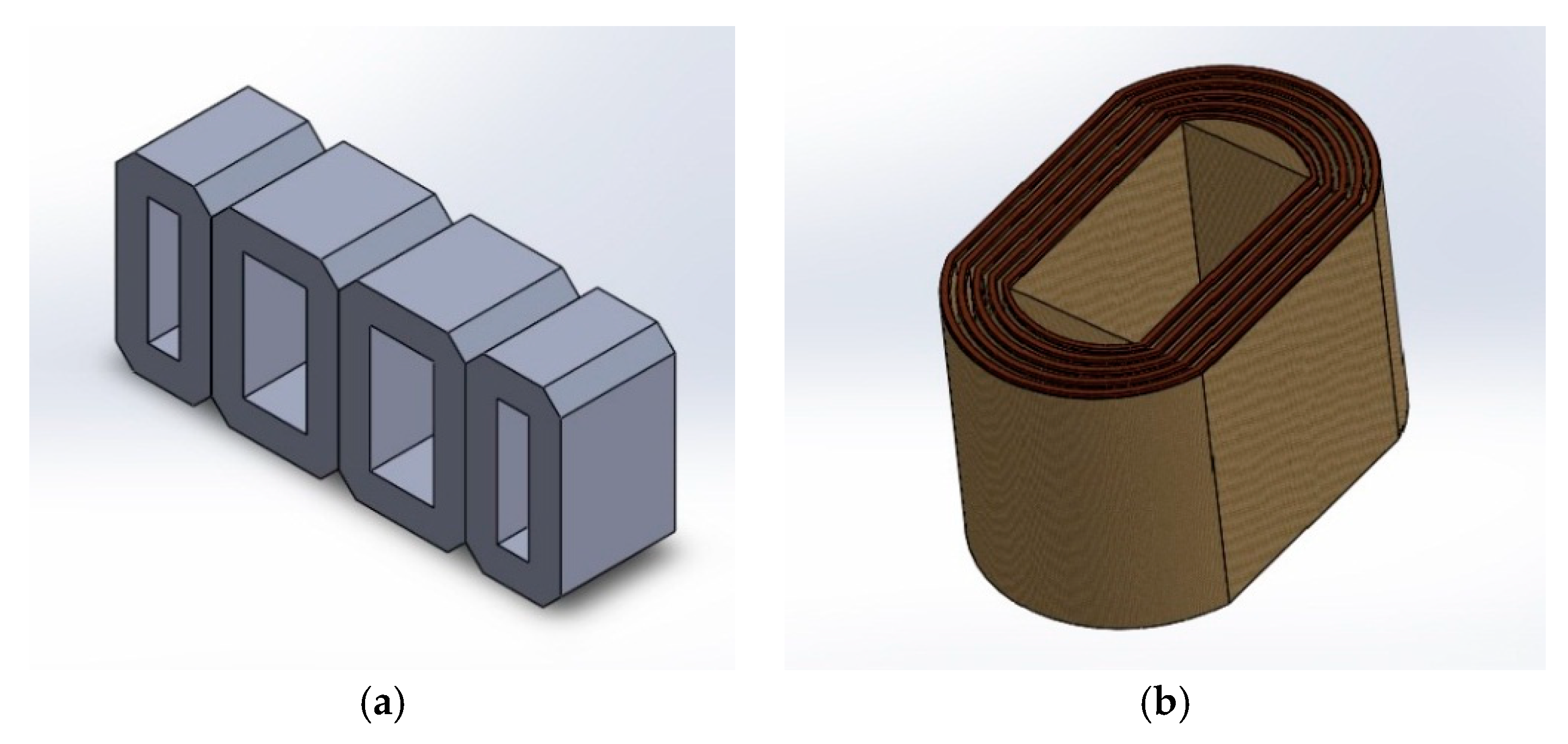
2.1. Thermal Model
2.2. Correlations for Free Convection
2.3. Numerical Solution
3. Experimental Procedure
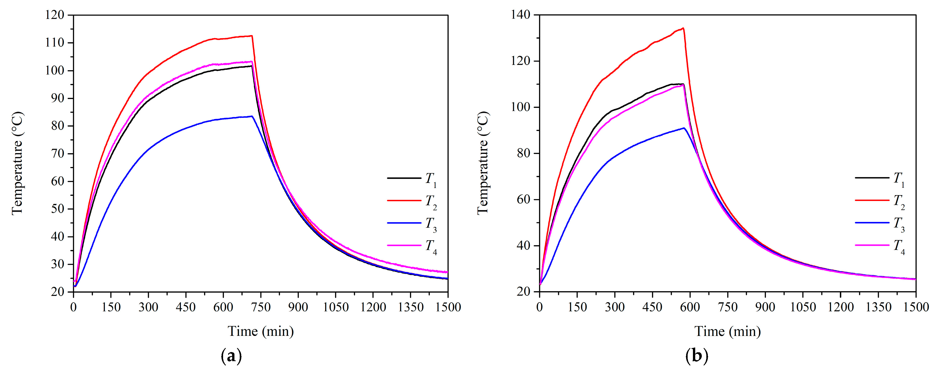
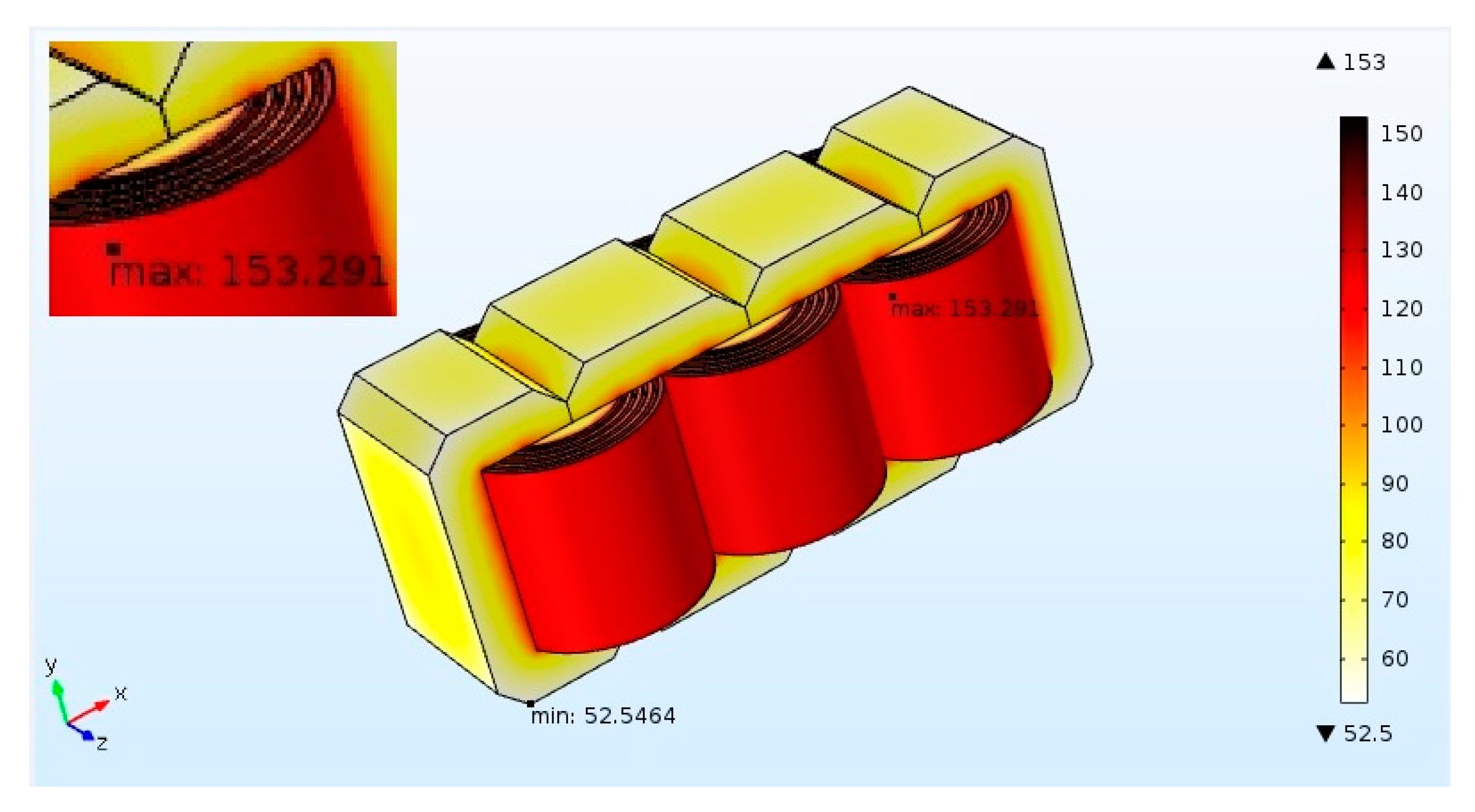
4. Result Analysis
5. Conclusions
Author Contributions
Funding
Acknowledgments
Conflicts of Interest
References
- Daut, I.; Syafruddin, H.S.; Ali, R.; Samila, M.; Haziah, H. The effects of harmonic components on transformer losses of sinusoidal source supplying non-linear loads. Am. J. Appl. Sci. 2006, 3, 2131–2133. [Google Scholar] [CrossRef]
- Amoda, O.A.; Tylavsky, D.J.; McCulla, G.A.; Knuth, W.A. Acceptability of three transformer hottest-spot temperature models. IEEE Trans. Power Deliv. 2012, 27, 13–22. [Google Scholar] [CrossRef]
- Sun, X.; Mu, Z. Analysis of hottest-spot temperature distribution in cast-resin dry-type transformer design. Adv. Mater. Res. 2012, 538–541, 1015–1019. [Google Scholar] [CrossRef]
- Vinet, L.; Zhedanov, A. IEEE Guide for Loading Mineral-Oil-Immersed Transformers and Step-Voltage Regulators; IEEE: Piscataway, NJ, USA, 2011. [Google Scholar] [CrossRef]
- Pierce, L.W. Predicting liquid filled transformer loading capability. IEEE Trans. Ind. Appl. 1994, 30, 170–178. [Google Scholar] [CrossRef]
- Zodeh, O.M.; Whearty, R.J. Thermal characteristics of a meta-aramid and cellulose insulated transformer at loads beyond nameplate. IEEE Power Eng. Rev. 1997, 17, 49–50. [Google Scholar] [CrossRef]
- Swift, G.W.; Zocholl, S.E.; Bajpai, M.; Burger, J.F.; Castro, C.H.; Chano, S.R.; Cobelo, F.; De Sa, P.; Fennell, E.C.; Gilbert, J.G.; et al. Adaptive transformer thermal overload protection. IEEE Trans. Power Deliv. 2001, 16, 516–521. [Google Scholar] [CrossRef]
- Swift, G.; Molinski, T.S.; Lehn, W. A fundamental approach to transformer thermal modeling—Part I: Theory and equivalent circuit. IEEE Trans. Power Deliv. 2001, 16, 171–175. [Google Scholar] [CrossRef]
- Susa, D.; Lehtonen, M.; Nordman, H. Dynamic thermal modelling of power transformers. IEEE Trans. Power Deliv. 2005, 20, 197–204. [Google Scholar] [CrossRef]
- Susa, D.; Lehtonen, M. Dynamic thermal modeling of power transformers: further development—Part II. IEEE Trans. Power Deliv. 2006, 21, 1971–1980. [Google Scholar] [CrossRef]
- Smolka, J.; Nowak, A.J. Experimental validation of the coupled fluid flow, heat transfer and electromagnetic numerical model of the medium-power dry-type electrical transformer. Int. J. Therm. Sci. 2008, 47, 1393–1410. [Google Scholar] [CrossRef]
- Lee, M.; Abdullah, H.A.; Jofriet, J.C.; Patel, D.; Fahrioglu, M. Air temperature effect on thermal models for ventilated dry-type transformers. Electr. Power Syst. Res. 2011, 81, 783–789. [Google Scholar] [CrossRef]
- Eslamian, M.; Vahidi, B.; Hosseinian, S.H. Analytical calculation of detailed model parameters of cast resin dry-type transformers. Energy Convers. Manag. 2011, 52, 2565–2574. [Google Scholar] [CrossRef]
- Ning, W.; Ding, X. Three-dimensional finite element analysis on fluid thermal field of dry-type transformer. In Proceedings of the 2012 Second International Conference on Instrumentation, Measurement, Computer, Communication and Control, Harbin, China, 8–10 December 2012; pp. 516–519. [Google Scholar]
- Tsili, M.A.; Amoiralis, E.I.; Kladas, A.G.; Souflaris, A.T. Power transformer thermal analysis by using an advanced coupled 3D heat transfer and fluid flow FEM model. Int. J. Therm. Sci. 2012, 53, 188–201. [Google Scholar] [CrossRef]
- Li, Y.; Guan, Y.J.; Li, Y.; Li, T.Y. Calculation of thermal performance in amorphous core dry-type transformers. Adv. Mater. Res. 2014, 986–987, 1771–1774. [Google Scholar] [CrossRef]
- Bulnes, F.; Tello, A.R.; Livera, M. Heat flux analysis in electrical transformers through integral operators of mechanics. Mod. Mech. Eng. 2014, 4, 84–107. [Google Scholar] [CrossRef]
- Barroso, R. Simulation and experimental validation of the core temperature distribution of a three-phase transformer. In Proceedings of the 2014 COMSOL Conference, Curitiba, Brasil, 23 October 2014. [Google Scholar]
- Rahimpour, E.; Azizian, D. Analysis of temperature distribution in cast-resin dry-type transformers. Electr. Eng. 2007, 89, 301–309. [Google Scholar] [CrossRef]
- Bergman, T.L.; Lavine, A.S.; Incropera, F.P.; DeWitt, D.P. Fundamentals of Heat and Mass Transfer; John Wiley & Sons: Hoboken, NJ, USA, 2011. [Google Scholar]
- Liao, R.; Zhang, F.; Yang, L. Electrical and thermal properties of kraft paper reinforced with montmorillonite. J. Appl. Polym. 2012, 126, E291–E296. [Google Scholar] [CrossRef]
- Magalhaes, E.D.; Silva, C.P.; Lima e Silva, A.L.; Lima e Silva, S.M. An alternative approach to thermal analysis using inverse problems in aluminum alloy welding. Int. J. Numer. Methods Heat Fluid Flow 2017, 27, 561–574. [Google Scholar] [CrossRef]


| Test | Number of Tetrahedral Elements | Winding 2 Temperature (°C) | Simulation Time (min) |
|---|---|---|---|
| A1 | 258,617 | 127.35 | 196 |
| A2 | 545,271 | 129.6 | 371 |
| A3 | 875,452 | 135.56 | 562 |
| A4 | 1,364,912 | 135.88 | 891 |
| A5 | 1,745,736 | 135.99 | 1274 |
| Thermocouple | Position | Coordinates (mm) |
|---|---|---|
| T1 | Winding 1 | (−100, −61, 45) |
| T2 | Winding 2 | (0, −61, 45) |
| T3 | Core surface | (0, 0, 0) |
| T4 | Winding 3 | (100, −61, 45) |
| Load | Temperature (°C) | Coordinates (mm) |
|---|---|---|
| Linear | 109.25 | (102.5, −63.43, 0.63) |
| Dynamic | 153.29 | (103, −63.43, 0.63) |
© 2018 by the authors. Licensee MDPI, Basel, Switzerland. This article is an open access article distributed under the terms and conditions of the Creative Commons Attribution (CC BY) license (http://creativecommons.org/licenses/by/4.0/).
Share and Cite
Mafra, R.G.; Magalhães, E.D.S.; Anselmo, B.D.C.S.; Belchior, F.N.; Lima e Silva, S.M.M. Winding Hottest-Spot Temperature Analysis in Dry-Type Transformer Using Numerical Simulation. Energies 2019, 12, 68. https://doi.org/10.3390/en12010068
Mafra RG, Magalhães EDS, Anselmo BDCS, Belchior FN, Lima e Silva SMM. Winding Hottest-Spot Temperature Analysis in Dry-Type Transformer Using Numerical Simulation. Energies. 2019; 12(1):68. https://doi.org/10.3390/en12010068
Chicago/Turabian StyleMafra, Rafael Gonçalves, Elisan Dos Santos Magalhães, Bruno De Campos Salles Anselmo, Fernando Nunes Belchior, and Sandro Metrevelle Marcondes Lima e Silva. 2019. "Winding Hottest-Spot Temperature Analysis in Dry-Type Transformer Using Numerical Simulation" Energies 12, no. 1: 68. https://doi.org/10.3390/en12010068
APA StyleMafra, R. G., Magalhães, E. D. S., Anselmo, B. D. C. S., Belchior, F. N., & Lima e Silva, S. M. M. (2019). Winding Hottest-Spot Temperature Analysis in Dry-Type Transformer Using Numerical Simulation. Energies, 12(1), 68. https://doi.org/10.3390/en12010068