Incremental State-Space Model Predictive Control of a Fresnel Solar Collector Field

Abstract

Model predictive control has been demonstrated to be one of the most efficient control techniques for solar power systems. An incremental offset-free state-space Model Predictive Controller (MPC) is developed for the Fresnel collector field located at the solar cooling plant installed on the roof of the Engineering School of Sevilla. A robust Luenberger observer is used for estimating the states of the plant which cannot be measured. The proposed strategy is tested on a nonlinear distributed parameter model of the Fresnel collector field. Its performance is compared to that obtained with a gain-scheduling generalized predictive controller. A real test carried out at the real plant is presented, showing that the proposed strategy achieves a very good performance.

1. Introduction

Currently, governments are promoting the use of renewable energy sources to reduce the environmental impact generated using fossil fuels [1,2]. Solar energy is, by far, the most abundant source of renewable energy. In fact, wind and most of the hydraulic energies come from solar energy [3,4]. The main application of the use of solar energy is producing electricity in solar thermal plants. A solar thermal plant is composed of a solar field which heats up a heat-transfer fluid (usually synthetic oil) to a desired temperature, a steam generator which uses the heated fluid to produce electricity, a storage system which provides energy when the solar field is not capable of doing it, and auxiliary elements such as valves, pipes etc. [1].

Many examples of solar thermal plants can be found. For instance, the three 50 MW Solaben and the two 50 MW Solacor parabolic-trough plants of Atlantica Yield in Spain, and the SOLANA and Mojave Solar parabolic-trough plant located at Arizona and California, each of 280 MW power production [5]. PS10 (10 MW), PS20 (20 MW) and Khi Solar One are examples of solar power plants operated by Atlantica Yield and Abengoa Solar respectively [6].

Another important application of solar energy is the supply of cold air for air conditioning in buildings. The use of solar energy for air conditioning is spurred by the fact that high demands of air conditioning correlates very well with the high levels of solar radiation [7,8].

This paper presents a control scheme designed for the Fresnel collector field which is a part of the solar cooling plant located at the Engineering School (ESI) of Seville [9,10]. This plant consists of a Fresnel collector field, a double-effect LiBr+ water absorption chiller and a storage tank. The water chiller is powered by hot pressurized water coming from the Fresnel solar field at 140–170 °C and produces air conditioning. When the solar radiation levels are not sufficient for reaching the required temperatures, the storage tank can be used. If the water temperature reaching the high temperature generator of the absorption machine is below 135 °C, the absorption machine uses natural gas.

In general, the control aim in solar plants is keeping the outlet temperature of the solar field as close as possible to a desired temperature set-point [11]. Since the decade of 1980, a considerable effort has been done concerning the development of control algorithm for solar power plants. Many of them were designed and tested for the experimental solar parabolic-trough plant of ACUREX at the plataforma solar de Almería [12]. For example, in [13,14] a review of different control strategies applied to the ACUREX plant is presented. In [15], an adaptative control scheme which cancels the resonance modes of the distributed collector field is presented. In [16], an observer-based MPC was developed and tested at the ACUREX field. In [17] a practical nonlinear MPC is designed. More recently, in [18] a nonlinear continuous-time generalized predictive control (GPC) applied to the distributed collector field ACUREX is presented and tested in simulation. In [19,20] different advanced control strategies using predictive and adaptative control strategies are described.

The linear Fresnel collectors can be used in multiple applications. For example, in [21] a model of a Fresnel collector field which uses molten salts as a heat-transfer fluid is presented. In [22], a model of a 100 MW solar power plant based on a linear Fresnel collector field is developed. In [23] a Fresnel collector field used in a desalination plant is described and the overall system efficiency is investigated.

Concerning the control of a Fresnel solar collector field, in [24,25] different control schemes for a Fresnel collector field are presented and an explicit MPC is developed and tested in a simulation environment. In [26], the modeling and control of a linear Fresnel collector system is addressed. In [27] a sliding model predictive control based on a feedforward compensation is developed and tested in simulation for a Fresnel collector field. More recently, in [28] a gain-scheduling generalized predictive controller is developed and tested at the real Fresnel plant described in this paper.

Since a solar collector field is affected by multiple disturbance sources and its dynamics changes strongly with the operating conditions [29,30], conventional linear control strategies do not perform well when the plant evolves far from the designing point [19]. In this paper, an incremental observer-based model predictive control algorithm is developed. The control strategy uses a linearization of the nonlinear distributed parameter model to obtain the linear models. The MPC algorithm uses an incremental formulation which ensures an offset-free response without using disturbance estimators as long as the reference is constant and reachable. Its performance is compared to that obtained with a gain-scheduling GPC [28]. The proposed control strategy shows faster tracking references.

Since only the inlet and outlet fluid temperatures are measurable, the intermediate temperatures as well as the metal temperatures must be estimated. The MPC strategy uses a robust Luenberger estimator. The estimator gain is obtained by a robust pole-placement technique allowing the imposition of stability constraints. The resulting problem can be solved via Linear Matrix Inequalities (LMI) considering a polytopic uncertainty of the plant. The main problem when using nonlinear estimators such as the unscented Kalman filter (UKF) is that imposing performance requirements and proving stability is a very difficult issue [31,32]. Furthermore, the stability of the MPC+UKF control strategy is still an open problem.

The paper is organized as follows: Section 2 describes the control objectives in solar power plants. Section 3 presents the solar cooling plant and describes its components. Section 4 presents the mathematical model of the Fresnel collector field used in this paper. Section 5 shows the design process of the proposed control strategy. Section 6 presents the simulation results, discussion of those results and the real tests performed at the real plant. Finally, Section 7 draws to a close with concluding remarks.

2. Control Objectives

The control objective in a solar energy plant is to maintain the outlet temperature of the solar field around a desired set-point [33]. To accomplish this objective, the water flow is used as a manipulated variable. This task is not an easy matter for two reasons:

• The system dynamics are very complex and highly nonlinear. Furthermore, the input-output delay changes with respect to the water flow. This fact produces that this kind of plants are very difficult to be controlled at low flow levels [34].
• The system is affected by multiple disturbance sources: inlet temperature, ambient temperature, solar time, solar radiation etc. The most important disturbance source is the solar radiation which can change suddenly because of passing clouds [29].

In general, the temperature set-point is chosen or computed according to optimal criteria [3]. The faster the controller can reach the desired set-point, the better. However, fast responses may excite the anti-resonance modes and high frequency dynamics of the system which lead to an oscillatory behavior [15]. For this reason, the controller should produce fast responses without exciting the high frequencies dynamics of the plant and reject properly the disturbances affecting the plant.

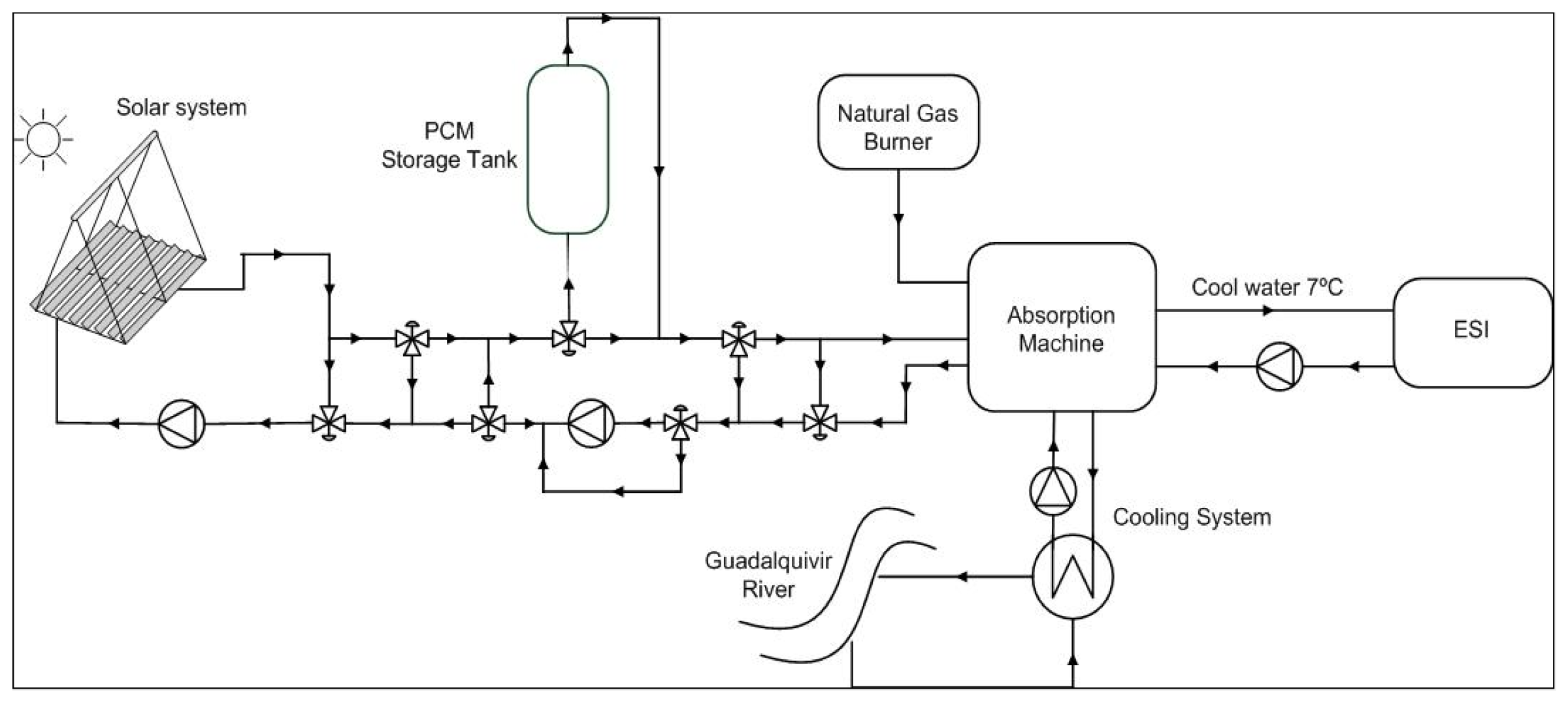
3. Plant Description

The solar cooling plant consists of three subsystems: the double-effect LiBr+ water absorption chiller of 174 kW nominal cooling capacity. The solar Fresnel collector field heats up the pressurized water and delivers it to the water absorption chiller. If the solar field cannot reach the required temperature for the absorption machine operation, the PCM storage tank can be used. Figure 1 shows the scheme of the whole plant.

Water absorption chiller: this is a double-effect cycle LiBr+ absorption machine with 174 kW and a theoretical COP of 1.34 [9]. The water chiller consists of three subsystems: (i) the high temperature generator which receives the hot water coming from the solar field (140–170 °C) and a nominal flow of 13 m³/h. If the temperature is not high enough, the absorption machine burns natural gas. (ii) the evaporator which cools down water from 14 °C to 7 °C with a nominal water flow of 30 m³/h. (iii) the refrigerator which dissipates the heat absorbed in the high temperature generator and the evaporator by transferring it to water from the Guadalquivir river at 30 °C and 37 m³/h of flow. For further information, the reader is referred to [35].

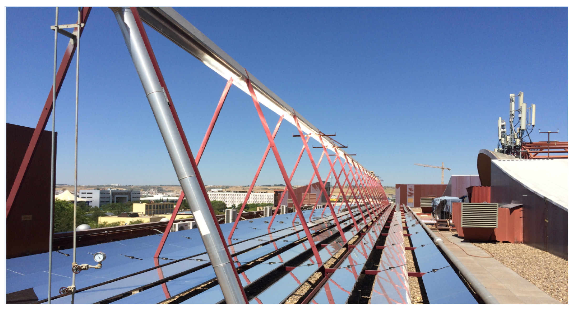
Solar Field: the solar field consists of a set of Fresnel solar collectors (see Figure 2) which concentrate the direct solar radiation onto the receiver tube placed in a plane parallel to the solar field. The metal tube is enveloped by a thin metal case called the secondary reflector. The secondary reflector aims at reflecting the solar beams which do not have direct impact on the receiver. The energy collected by the receiver tube is then transferred to a heat-transfer fluid (in our case, pressurized water).

The solar field orientation is East-West, and the sun-tracking system modifies the inclination of every row to concentrate the sun beam onto the metal tube. To do this, the sun-tracking system computes the solar vector by using the well-known formulas for solar azimuth and solar height [1], and then calculates the desired inclination of every row using the relative position between the row and the tube as explained in [10].

To change the flow provided by the water pumps, the pump speed variation must be used. Since the control signal provided by the control algorithm proposed here is the water flow, an intermediate PID controller is used. It receives the water flow set-point and modifies the speed variator accordingly to obtain it.

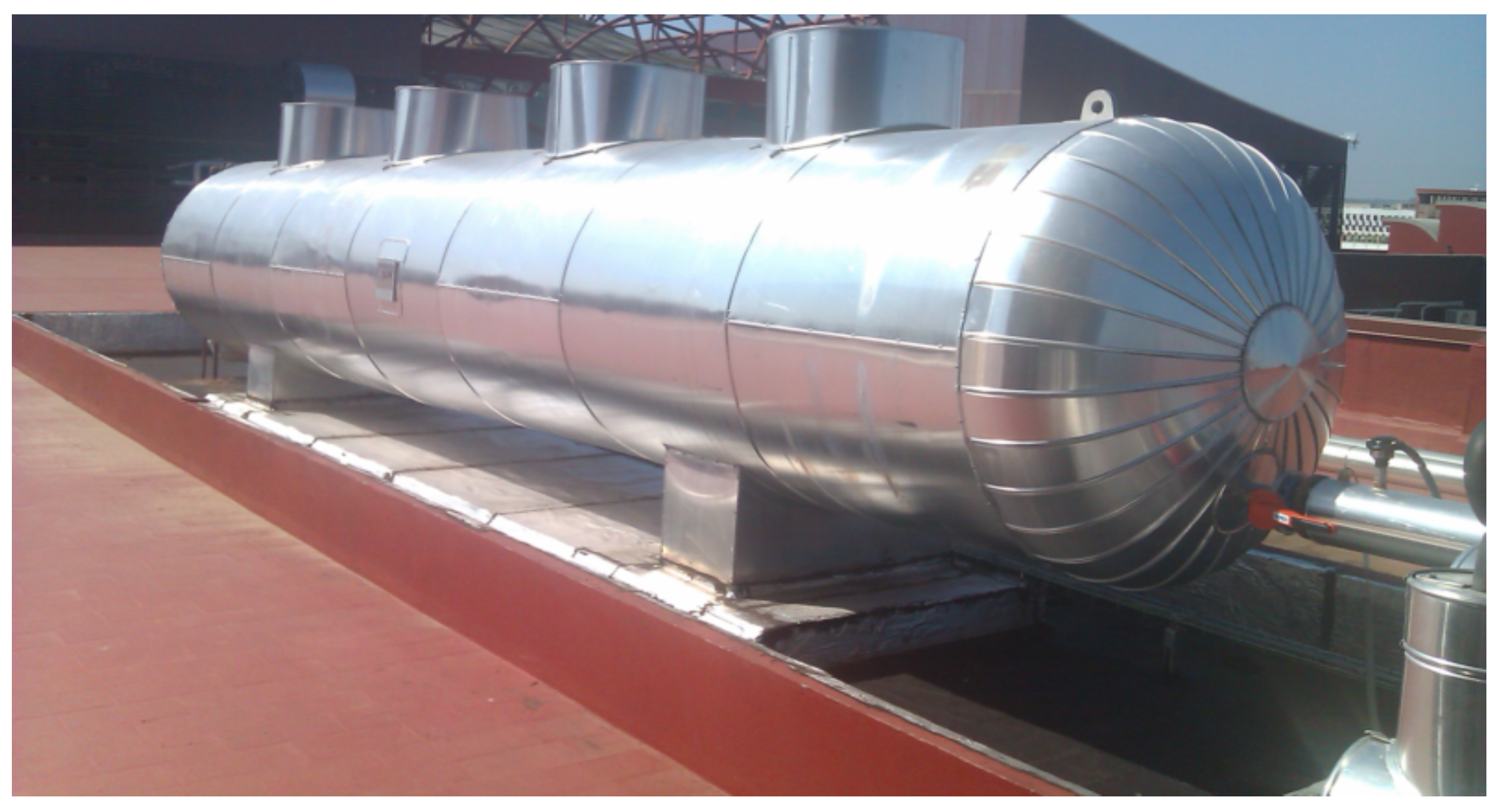
PCM storage tank: The PMC storage is a tank of 18 m long and 1.31 m of diameter (Figure 3). The storage tank is a shell-tube heat exchanger with a theoretical thermal storage capacity of 275.5 kWh (145–180 °C) and 150 kW. It consists of a series of tubes containing a heat-transfer fluid and the PCM fills up the space between tubes and the shell. The theoretical thermal storage is computed by using the properties of the hydroquinone. The total mass of the PCM is of 3294 kg [36]. The melting temperature of the hydroquinone is about 170 °C which is suitable for the water absorption chiller operating range [37].

4. Mathematical Modeling of the Fresnel Collector Field

A mathematical model of the Fresnel collector field has been developed using similar equations to those obtained for parabolic-trough fields [12] but taking into account a different way of computing the geometrical efficiency and the shading factor.

Two different models are used [38]: concentrated parameter model which is usually used for feedforward control purposes and the distributed parameter model used for simulating the performance of the closed-loop control strategies.

4.1. Distributed Parameter Model

The Fresnel solar collector field consists of a set of Fresnel solar collectors which concentrate solar radiation onto a line where an absorption tube of 64 m long is located. The model is described by the following system of partial differential equations (PDE) describing the energy balance [39]:

$$\begin{gathered} {\rho }_m{C}_m{A}_m\frac{\partial T_m}{\partial t}=I{K}_{opt}no{G}_a-H_l{G}_a(T_m-T_a)-l_p{H}_t(T_m-T_f) \\ {\rho }_f{C}_f{A}_f\frac{\partial T_f}{\partial t}+{\rho }_f{C}_{f}q\frac{\partial T_f}{\partial l}=l_p{H}_t(T_m-T_f) \end{gathered}$$

(1)

where m subindex refers to metal and f subindex refers to a fluid. In

Table 1. Parameters description.

Symbol	Description	Units
t	Time	s
l	Space	m
$T(x,t)$	Temperature	K,°C
$q\left(t\right)$	Water flow rate	m3s−1
$\rho (t,T)$	Density	kgm−3
$C(t,T)$	Specific heat capacity	JK−1kg−1
A	Cross-sectional area	m2
$I\left(t\right)$	Direct Solar Radiation	Wm−2
$no\left(t\right)$	geometric efficiency	Unitless
$K_{opt}$	Optical efficiency	Unitless
$G_a$	Collector aperture	m
$T_a\left(t\right)$	Ambient temperature	K,°C
$H_l(t,T)$	Global coefficient of thermal loss	Wm−2°C−1
$H_t(t,T,q)$	Coefficient of heat transmission metal-fluid	Wm−2°C−1
$l_p$	Length of pipe line	m
S	Total reflective surface	m2
$C_T(t,T)$	Thermal capacity of the solar field	J/K
$P{c}_p(t,T)$	Parameter of solar field	J m−3K−1

, parameters and their units are shown.

The PDE system is solved by dividing the metal and fluid in 64 segments of 1 m long. The chosen integration step is 0.5 s. The equations are integrated by using an Euler method.

The geometric efficiency depends on the solar time. It takes into account the effect of the cosine of the incidence angle of the solar beam and the shade factor. Its computation involves complex trigonometric formulas. These are well explained in [10].

Some parameters have been adjusted using real data from the real solar field. In particular, the density, specific heat, coefficient of heat transmission have been obtained as polynomial functions of the segment temperature and the water flow using thermodynamic data of pressurized water. The coefficient of thermal losses has been obtained using real data from the Fresnel solar field. Their expressions are given by Equations (2)–(4):

$${\rho }_f=-0.0025T_f^2-0.203T_f+1003.91$$

(2)

$$C_f=5.16e-7T_f^4-1.56e-4T_f^3+0.0277T_f^2-1.627T_f+4207.403$$

(3)

$$\begin{gathered} H_v=1.34e-4T_f^4-7.78e-2T_f^3+18.73T_f^2-2.57e3T_f+4.11e5 \\ {H}_t=H_v{q}^{0.8} \end{gathered}$$

(4)

The thermal losses coefficient can be calculated using Equation (5):

$$H_l=\left(0.00122\right)(T_m-T_a)+0.001763$$

(5)

4.2. Concentrated Parameter Model

The concentrated parameter model provides a lumped description of the whole field. The variation in the internal energy of the fluid can be described by the equation [10]:

$$C_T\frac{d{T}_{out}}{dt}=K_{opt}noSI-qP{c}_p(T_{out}-T_{in})-H_{l}S(\overline{T}-T_a)$$

(6)

where q is the water flow, $T_{out}$ and $T_{in}$ are the outlet and inlet oil temperatures, respectively. $\overline{T}$ is the average value between inlet and outlet temperatures and $T_a$ is the ambient temperature. $C_T$ is the thermal capacity of the solar field, $K_{opt}$ is the optical efficiency (which incorporates the effects of mirror reflectivity, tube absorptance, interception factor), I is the solar irradiance and S is the total reflective surface measuring 352 m². The geometric efficiency $no$ is a function of the cosine of the incidence angle between the mirrors’ normal vector and the solar beam and the shade factor, $P{c}_p$ takes into account some geometrical and thermal properties of the loop and $H_l$ is the coefficient of thermal losses.

4.3. Comparison between Real Data and Models Output

Figure 4 and Figure 5 show the comparison between the model output and the real outlet temperature from solar field. As can be seen, the model dynamics is very similar to that of the real plant.

To show a comparison between the evolution of the distributed parameter model and the lumped parameter model is shown in Figure 6. Figure 7 shows the evolution of the error between the output of the models and the real outlet temperature. As can be seen the distributed model achieves better results as expected.

5. Model Predictive Control Strategy

In this section, the observer-based state-space MPC is presented. The state-space matrices used by the MPC are obtained by means of the distributed parameter model (1). The linear model is obtained by dividing the absorption metal tube into 4 segments (instead of the 64 used in the full distributed nonlinear model). This simplification allows to reduce the complexity of the control strategy and thus the computational time is also diminished.

Since only the inlet and the outlet temperature of the fluid are available, the temperatures of metal segments and fluid in the intermediate sections must be estimated. The state estimator is a robust Luenberger state-observer. The observer gain is computed using a robust pole placement via LMI considering a polytopic uncertainty of the plant dynamic [40]. Using this approach, the stability of the state observer is ensured by imposing stability and performance conditions to the closed-loop poles in the z plane [41].

5.1. MPC Problem

Basically, an MPC control algorithm consists of the following 3 steps [42,43]:

• Use a model to predict the process evolution at future time instants (horizon), depending on a control sequence.
• Compute the control sequence which minimizes a certain objective function.
• Apply only the first element of the control sequence, then in the rest of sampling instants recalculate the sequence shifting the horizon one step in the future (receding horizon). Repeat steps 1 to 3.

The use of a conventional linear controller in a plant with highly nonlinear dynamics presents some drawbacks. The performance of linear controllers may deteriorate if the state of the plant evolves far from the design point. In systems such as Fresnel collector or Parabolic-trough plants, the dynamics of the plant becomes complex at low water flows [44]. To overcome this drawback, in this paper the linear model is computed each sampling time. The sampling time is chosen as 20 s, selected by taking into account the time characteristics of closed-loop time constants. Augmenting the sampling time would produce slower reactions by the control algorithm and it is not desirable. Diminishing the sampling time may produce faster reactions of the controller but the high dynamics modes of the solar field may be excited as shown in [16]. Furthermore, the sampling time cannot be smaller than 10 s due to communication requirements of the data acquisition system.

In general, the mathematical expression of the MPC problem can be posed as follows:

$$\underset{\mathrm{\Delta }u}{min}J=\sum _{t=1}^{N_p}{\left(y_{k+t|k}-y_{k+t}^{ref}\right)}^{⊺}\left(y_{k+t|k}-y_{k+t}^{ref}\right)+R_u\sum _{t=0}^{N_c-1}\mathrm{\Delta }{u}_{k+t|k}^{⊺}\mathrm{\Delta }{u}_{k+t|k}$$

(7)

s.t.

$$\begin{array}{cc}\hfill y_{k+t|k}& =f(\mathrm{\Delta }u,y_{k+t-1},y_{k+t-2},\dots )\hfill \\ \hfill u_{k+t|k}& =u_{k+t-1|k}+\mathrm{\Delta }{u}_{k+t|k}\hfill \\ \hfill u_{min}& \le u_{k+t|k}\le u_{max}\hfill \\ \hfill t& =0,\dots ,N_p-1\hfill \end{array}$$

(8)

where $N_p$ and $N_c$ stand for the prediction and the control horizons, respectively. The parameter $R_u$ penalizes the control effort. Then $u_k\equiv u_{k|k}$ is applied to the system. In this case, only constraints in the amplitude of the water flow have been considered.

5.2. Obtaining the Linear Models

The linear model of the PDE system (1) consists of a set of matrices depending of inputs and system states. Let x be the state vector formed by the temperatures of the 4 metal and fluid segments, $T_{in}$ the inlet temperature, q the water flow, $I_e=I{K}_{opt}{n}_o$ the effective solar radiation, and $T_a$ the ambient temperature. $\mathrm{\Delta }l$ is the length of each segment in which the metal tube is broken down (16 m).

The linear model in continuous time is computed using (9):

$$\begin{gathered} {\dot{x}}_t=A{x}_t+B{u}_t+B_d{d}_t \\ {y}_t=C{x}_t \end{gathered}$$

(9)

$$u_t=q{d}_t={\left[\begin{array}{ccc}{T}_{in}& I_e& T_a\end{array}\right]}^{⊺}$$

(10)

The linear matrices are computed as follows:

$$\begin{array}{cc}{P}_0=\frac{-H_l{G}_a-l_p{H}_t}{{\rho }_m{C}_m{A}_m}\hfill & \hfill P_1=\frac{l_p{H}_t}{{\rho }_m{C}_m{A}_m}\end{array}$$

(11)

$$\begin{array}{cc}{P}_2=\frac{l_p{H}_t}{{\rho }_f{C}_f{A}_f}\hfill & \hfill P_3=\frac{q}{A_f\mathrm{\Delta }l}\end{array}$$

(12)

$$\begin{array}{c}{P}_4=-P_2-P_3\hfill \end{array}$$

(13)

$$A=\left(\begin{array}{cccccccc}{P}_0& 0& 0& 0& P_1& 0& 0& 0\\ 0& P_0& 0& 0& 0& P_1& 0& 0\\ \dots & \dots & \dots & \dots & \dots & \dots & \dots & \dots \\ 0& 0& 0& P_0& 0& 0& 0& P_1\\ P_2& 0& 0& 0& P_3& 0& 0& 0\\ 0& P_2& 0& 0& P_4& P_3& 0& 0\\ \dots & \dots & \dots & \dots & \dots & \dots & \dots & \dots \\ 0& 0& 0& P_2& 0& 0& P_4& P_3\end{array}\right)$$

(14)

where the first 4 states correspond to the metal temperatures and the other 4 correspond to the fluid temperatures. It is worth noting that the value of the control signal q appearing in the matrix A is the value defining the operating point around the nonlinear model is linearized.

$$B={\left[\begin{array}{cccc}{0}_{1x4}& \frac{1}{A_f\mathrm{\Delta }l}& \dots & \frac{1}{A_f\mathrm{\Delta }l}\end{array}\right]}^{⊺}$$

(15)

$$B_{Tin}={\left[\begin{array}{ccc}{0}_{1x4}& \frac{q}{A_f\mathrm{\Delta }l}& 0_{1x3}\end{array}\right]}^{⊺}$$

(16)

$$B_{Ie}={\left[\begin{array}{cc}{1}_{1x4}·\frac{G_a}{{\rho }_m{C}_m{A}_m}& 0_{1x4}\end{array}\right]}^{⊺}$$

(17)

$$B_{Ta}={\left[\begin{array}{cccc}\frac{H_l{G}_a}{{\rho }_m{C}_m{A}_m}& \dots & \frac{H_l{G}_a}{{\rho }_m{C}_m{A}_m}& 0_{4x1}\end{array}\right]}^{⊺}$$

(18)

$$B_d={\left[\begin{array}{ccc}{B}_{Tin}& B_{Ie}& B_{Ta}\end{array}\right]}^{⊺}$$

(19)

$$C=\left[\begin{array}{cccccccc}0& 0& 0& 0& 0& 0& 0& 1\end{array}\right]$$

(20)

Notice that A and $B_{Ta}$ matrices depend on the system states, water flow and parameters; $B_{Tin}$ is function of the water flow u.

The variables ${\rho }_m$, $C_m$, $A_f$, $A_m$ and G are constants whereas each parameter $H_l$, $p_f$, $C_f$ and $H_t$ depend on the state temperature and are calculated around the operation point in which the plant is working at. The linear matrices are discretized using a sampling time of 20 s. In the remainder we will refer to the discrete-time matrices keeping the notation A, B and $B_d$.

5.3. Computation of the Observer Gain

As stated above, only the inlet and outlet fluid temperatures are measured in this plant. Since the intermediate fluid temperatures and the metal segments temperature are needed for the MPC, they must be estimated. A Luenberger observer is implemented and the observer gain L is obtained by the solution of a LMI problem.

The advantage of using the Luenberger observer is that performance constraints can be imposed. This fact allows not only ensuring the stability of the observer for the whole range of the plant dynamics, but it also allows to impose dynamics behavior. To fulfill this aim, a polytopic Linear Differential Inclusion (LDI) description of plant is used. A 36-vertex polytope is employed, representing the behavior inside the range of water flow, operative temperature, and direct solar radiation.

In this kind of systems, the dynamics is mainly dictated by the flow and the direct solar radiation [11,19], although other variables have also influence: the optical and geometrical efficiencies, the inlet and outlet temperatures etc. To obtain a representative set of linear systems representing the dynamics of the solar field, 36 linear systems are chosen for simplicity. Otherwise the polytope contains a very high number of vertices depending on different operating conditions. This fact proves that solving the LMI problem becomes more difficult and computationally heavier.

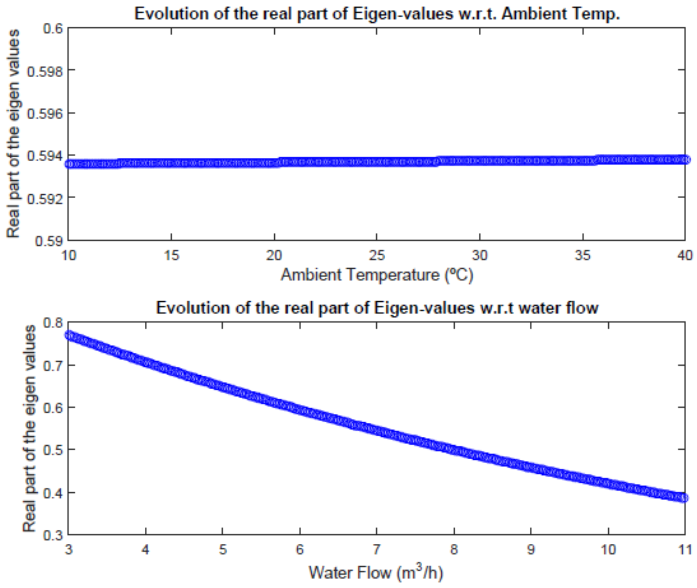
In this paper, four values for the water flow are considered: 3.5, 6, 8.7 and 11 m³/h. Three values for the direct solar radiation (low, medium, and high) are taken into account: 300, 600 and 950 W/m². The values of the effective solar radiation are obtained considering two values of the direct solar radiation (950 W/m² and 350) and a typical value of the overall efficiency of 0.35. As far as the inlet temperature is concerned, three values are considered covering the range of working temperature: 40, 80 and 140 °C. The ambient temperature is considered to be 25 °C. It has been found that the ambient temperature, which is used to compute the thermal losses to the ambient, has an almost negligible influence in the system dynamics. For this reason, this is considered to be a typical value of 25 °C. The variation of the matrix A eigenvalues depends much more on the water flow than on the ambient temperature. It can be seen in Figure 8: the upper part shows the evolution of the real part of the fluid segments eigenvalues with respect to the ambient temperature. The inlet temperature is considered to be 120 °C and the direct solar radiation is considered to be 900 W/m². As seen, the evolution of the eigenvalues in the upper part of Figure 8 is almost constant, in other words, the dependence of the dynamics with respect to the ambient temperature is almost negligible. However, the evolution with respect to the water flow showed in the bottom part is much more important.

The value of the states to compute the corresponding linear matrices are obtained by solving the nonlinear distributed parameter model equations in steady-state. Thus, when the 36 systems are computed, the observer gain can be obtained.

The equations describing the dynamics of the estimated state (in discrete time) are given by:

$$\begin{gathered} {\widehat{x}}_{k+1}=A(k,x,u){\widehat{x}}_k+B{u}_k+B_d{d}_k+L\left({\widehat{y}}_k-y_k\right) \\ \widehat{y}(k+1)=C{\widehat{x}}_k \end{gathered}$$

(21)

where $A(k,x,u)\in \mathbf{Co}\left\{A_1,\dots ,A_4\right\}$.

The estimation error is defined as $e_k={\widehat{x}}_k-x_k$ and its dynamics is given by:

$$e_{k+1}=\left(A(k,x,u)+LC\right)e_k$$

(22)

The objective of the LMI problem formulated here is to find an observer gain matrix L such that $e\left(k\right)$ converges to zero for $k\to \infty$ with the system described by the polytopic LDI, with the performance requirements imposed by pole clustering constraints. Notice that to avoid nonlinear terms in the LMI, we formulate the problem on ${\left(A(k,x,u))+LC\right)}^{⊺}$ exploiting the fact that a square matrix shares the same eigenvalues with its transpose.

This translates in searching for a positive definite matrix W such that the following LMIs are satisfied for each vertex of the polytope [45].

$$\begin{gathered} \underset{W,Y}{min}r \\ {A}_i^{⊺}W+C^{⊺}Y+WA+Y^{⊺}C>0 \end{gathered}$$

(23a)

$$\left[\begin{array}{cc}-rW& A^{⊺}W+C^{⊺}Y\\ WA+Y^{⊺}C& -rW\end{array}\right]<0$$

(23b)

with $Y=L^{⊺}W$ and $r\in (0,1)$, which correspond to the following conditions for pole clustering [40,46]:

• $\mathbf{Re}\left(\lambda (A_i+LC)\right)>0$
• $\left|\lambda (A_i+LC)\right|<r$

Notice that as the condition in (23b) constitutes a Bilinear Matrix Inequalities (BMI). The simplest method to solve the LMI problem is choosing the value of r as a constant and scaling it iteratively by a factor $\beta <1$. The LMI problem is solved while it is feasible.

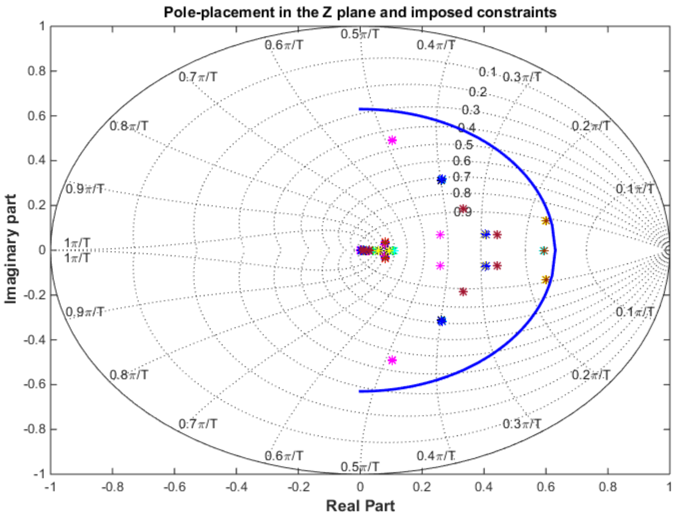
Figure 9 shows the poles of the observer for the 36 linear systems considered. It can be seen that they are inside the constraint region ensuring not only stability but also appropriate dynamic behavior. The minimum radius obtained was 0.62.

5.4. Offset-Free State-Space MPC

In this subsection, the incremental formulation of the state-space formulation is presented.

In general, when using state-space formulation in model predictive control strategies, steady-state errors may appear due to modeling errors or plant model mismatches. This problem has been addressed in literature by including a disturbance estimator to compensate model-plant mismatches [47,48]. The drawback of this approach is that additional dynamics is added to the controller and the parameters to be tuned increase. The approach considered in this paper, is using and incremental formulation of the MPC problem [49]. This formulation achieves offset-free tracking of constant references for systems without a zero in the origin. Subsequently, a brief description of the procedure is given, since the complete analysis can be found in [49].

Considering a linear state-space model with n states, m outputs, r inputs and p disturbance sources:

$$\begin{gathered} x_{k+1}=A{x}_k+B{u}_k+B_d{d}_k \\ {y}_k=C{x}_k \end{gathered}$$

(24)

The key is to use an incremental form of the state-space formulation and augmenting the states to include the system output [49]. The incremental formulation is described as follows:

$$\mathrm{\Delta }{x}_{k+1}=A\mathrm{\Delta }{x}_k+B\mathrm{\Delta }{u}_k+B_d\mathrm{\Delta }{d}_k$$

(25)

$$y_k=y_{k-1}+C\mathrm{\Delta }{x}_k$$

(26)

where $\mathrm{\Delta }{x}_k=x_k-x_{k-1}$. Augmenting Equations (25) and (26), the complete state-space model is posed as follows:

$$\stackrel{{\tilde{x}}_{k+1}}{\overbrace{\left[\begin{array}{c}\mathrm{\Delta }{x}_{k+1}\\ y_k\end{array}\right]}}=\stackrel{\tilde{A}}{\overbrace{\left[\begin{array}{cc}A& 0_{n\times m}\\ C& I_{m\times m}\end{array}\right]}}\stackrel{{\tilde{x}}_k}{\overbrace{\left[\begin{array}{c}\mathrm{\Delta }{x}_k\\ y_{k-1}\end{array}\right]}}+\stackrel{\tilde{B}}{\overbrace{\left[\begin{array}{c}B\\ 0_{m\times r}\end{array}\right]}}\mathrm{\Delta }{u}_k+$$

(27)

$$\stackrel{\widetilde{Bd}}{\overbrace{\left[\begin{array}{c}Bd\\ 0_{p\times r}\end{array}\right]}}\mathrm{\Delta }{d}_k$$

(28)

$$y_k=\stackrel{\tilde{C}}{\overbrace{\left[\begin{array}{cc}C& I_{m\times m}\end{array}\right]}}\left[\begin{array}{c}\mathrm{\Delta }{x}_k\\ y_{k-1}\end{array}\right]$$

(29)

The new matrices can be used in the MPC control algorithm to obtain the desired control signal at instant k. The difference with the standard state-space MPC formulation is that the free response of the system depends on the measurement of $y_{k-1}$ producing an offset-free tracking of references [49]. The new system can be posed as follows:

$${\tilde{x}}_{k+1}=\tilde{A}{\tilde{x}}_k+\tilde{B}\mathrm{\Delta }{u}_k+\widetilde{Bd}\mathrm{\Delta }{d}_k$$

(30)

$$y_k=\tilde{C}{\tilde{x}}_k$$

(31)

The predicted response can be obtained as the sum of the forced response, the term that depends on the future control actions, and the free response which does not depend on the future control actions [42] as follows:

$$y=G\mathrm{\Delta }u+f$$

(32)

The matrix G can be obtained from the model matrices (Equations (30) and (31)) and the free response can be computed as a matrix depending on the past values of the states, outputs, and measured disturbances. Since it is difficult to know how disturbances are going to evolve in the future, they are assumed to be constant along the prediction horizon. The free response can be calculated as follows [42]:

$$f=F\left[\begin{array}{c}\mathrm{\Delta }{\tilde{x}}_k\\ y_{k-1}\end{array}\right]+G_{Ie}\mathrm{\Delta }{I}_e+G_{Tin}\mathrm{\Delta }Tin+G_{Ta}\mathrm{\Delta }{T}_a$$

(33)

The matrix F can be obtained from the model, and the matrices $G_{Ie}$, $G_{Ta}$ and $G_{Tin}$ are the contribution of the effective solar radiation, the ambient temperature, and the inlet temperature to the free response.

5.5. Final Control Scheme

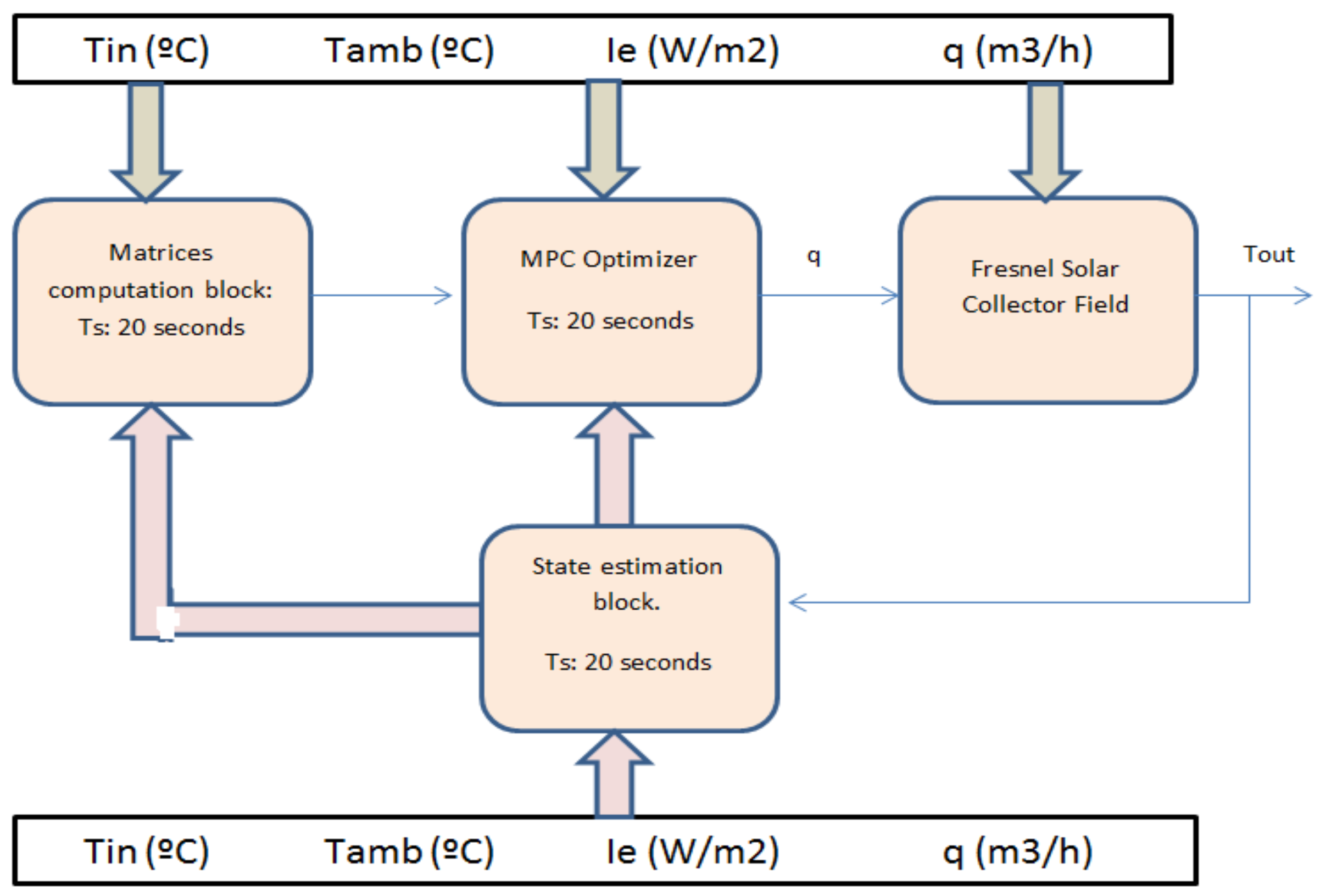
In this subsection, the final control scheme is presented. Every 20 s the data acquisition system takes the data from the field and the state observer computes the estimated states. This estimation is provided to the block which computes the linear matrices and solves the MPC problem given by Equation (8). The MPC optimizer computes a control signal, q, which is applied to the Fresnel collector field. Figure 10 shows this control scheme:

6. Simulation Results, Discussion and Experimental Results

In this section, some simulation results are presented comparing the proposed control strategy with a Gain-Scheduling Generalized Predictive Controller (GS-GPC). This controller was tested in simulation and in the real plant and it provided very good performance. In this paper, the GS-GPC control strategy is outlined. For further information, the reader is referred to [28]. Another important point is that the data used for simulation purposes is taken from the real Fresnel collector field.

A gain-scheduling controller is an easy way to cope the changing dynamics of a nonlinear system. Since a linear controller is tuned to a particular working point, when the plant evolves far from the design conditions, the linear controller performance may deteriorate. A gain-scheduling approach is an easy way to deal with the changing dynamics of the plant depending on the operating conditions. The GS-GPC control strategy uses a series feedforward to linearize the plant and to cope with measurable disturbances [50]. The feedforward is computed using the concentrated parameter model as follows:

$$q=\frac{(K_{opt}noSI-H_{l}S(\overline{T}-T_a))}{qP{c}_p(Tre{f}_{vir}-T_{in})}$$

(34)

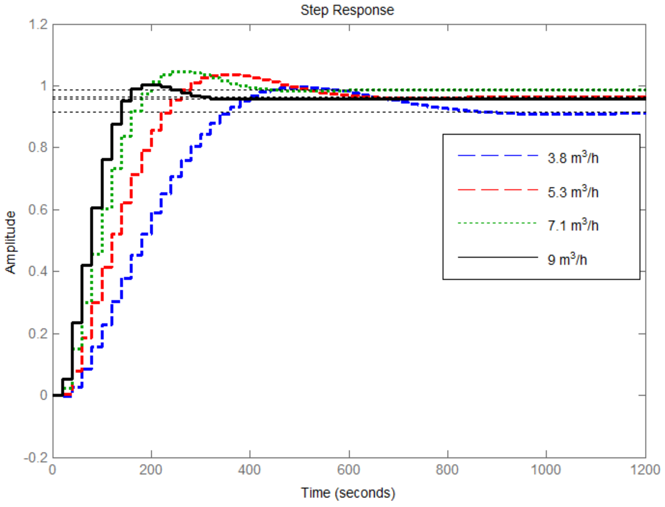
In this case, the dynamics of the plant depends mainly on the water flow as stated in [51]. Four water flow level are considered covering the range of operation (3.8–9.1 m³/h). For each water flow level, a discrete transfer function is obtained as follows (Equation (35)):

$$G\left(z^{-1}\right)=\frac{b_o+b_1{z}^{-1}+b_2{z}^{-2}+b_3{z}^{-3}+b_4{z}^{-4}}{1+a_o{z}^{-1}+a_1{z}^{-2}}$$

(35)

Figure 11 shows the step response for different water flow conditions. The linear model parameters are interpolated for intermediate flow values. Every sampling time (20 s), a transfer function is obtained, and a GPC optimization problem is solved [28]. The parameters for the GS-GPC are chosen as follows: the control horizon $N_c=7$, the prediction horizon $N_p=12$ and $\lambda$ = 6.

The tuning parameters of the MPC are chosen as $N_c=8$, $N_p=14$ and $R_u=2e8$. The water flow can vary from 3 to 10 m³/h for simulation purposes. The value of $R_u$ is high because the cost function is not normalized.

6.1. Simulation Results

In this subsection, two simulation are carried out comparing the response of the two controllers, the GS-GPC and the MPC.

Figure 12 shows the first simulation consisting of a series of changing set-points for the outlet temperature. The direct solar radiation corresponds to a clear day with passing clouds. The data to carry out the simulation corresponds to the day 29 June of 2009. The temperature reference is initially at 120 °C. Then a series of increasing steps in the reference temperature are selected. The MPC controller provides slightly faster responses with very small overshoots. Both controllers reject properly the disturbances in the solar radiation and the inlet temperature. As can be seen, an offset-free tracking response is obtained in the proposed control strategy.

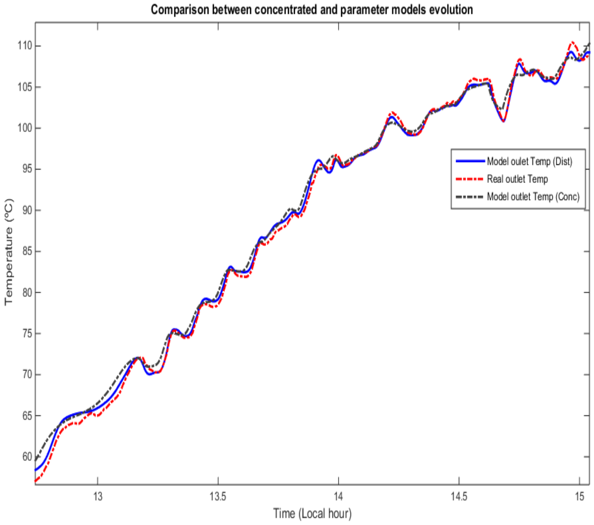
Figure 13 depicts the comparison between the temperature profiles obtained by the robust Luenberger observer and those provided by the distributed parameter model. As seen, the estimated profiles follow the dynamics of the real measurements properly. Small steady-state errors appear due the loss of precision produced for considering a smaller number of segments in the linear model (4 for fluid and metal temperatures) than those considered in the distributed parameter model (64 segments for fluid and metal temperatures). The maximum error observed in about 1 °C.

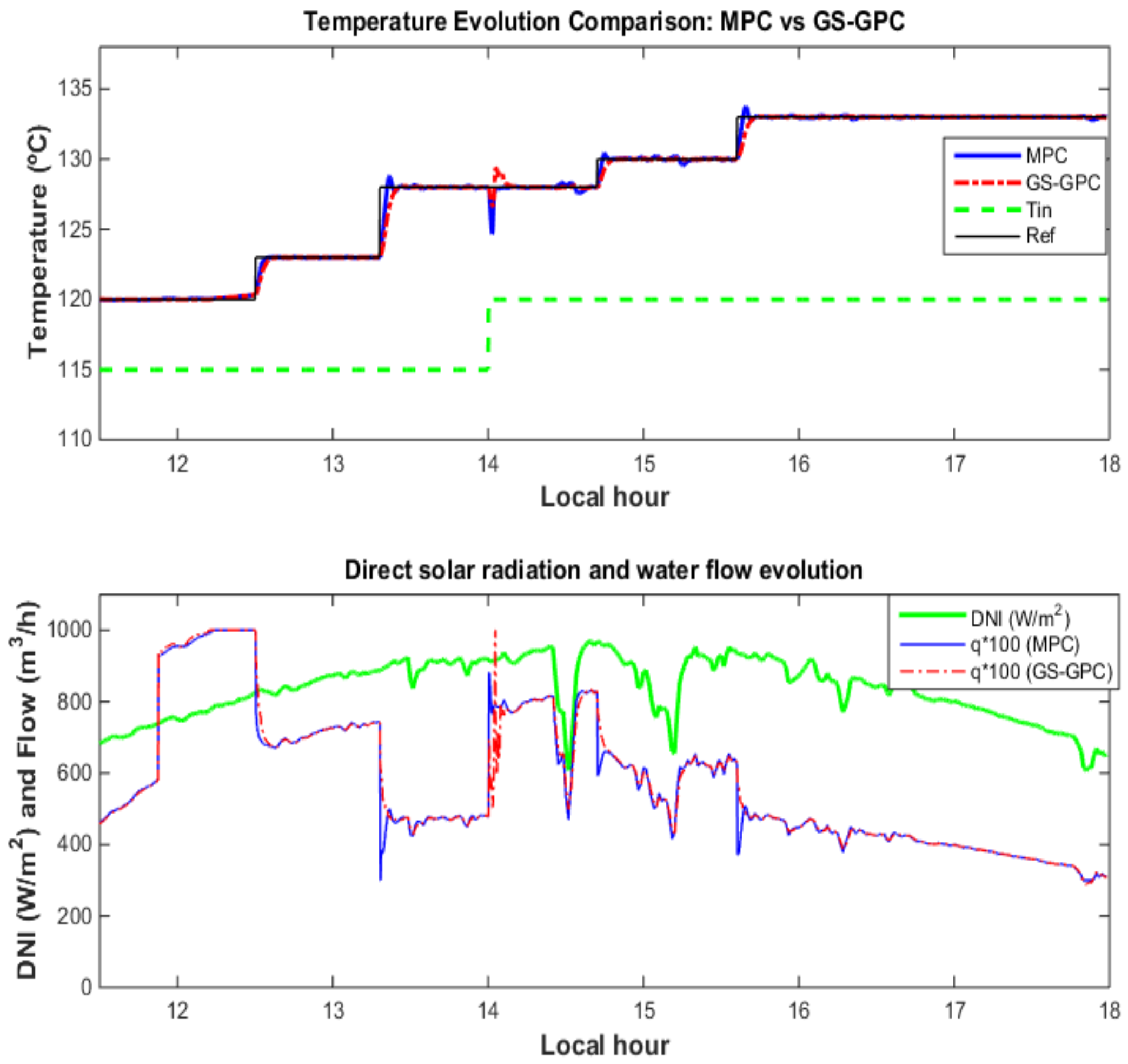
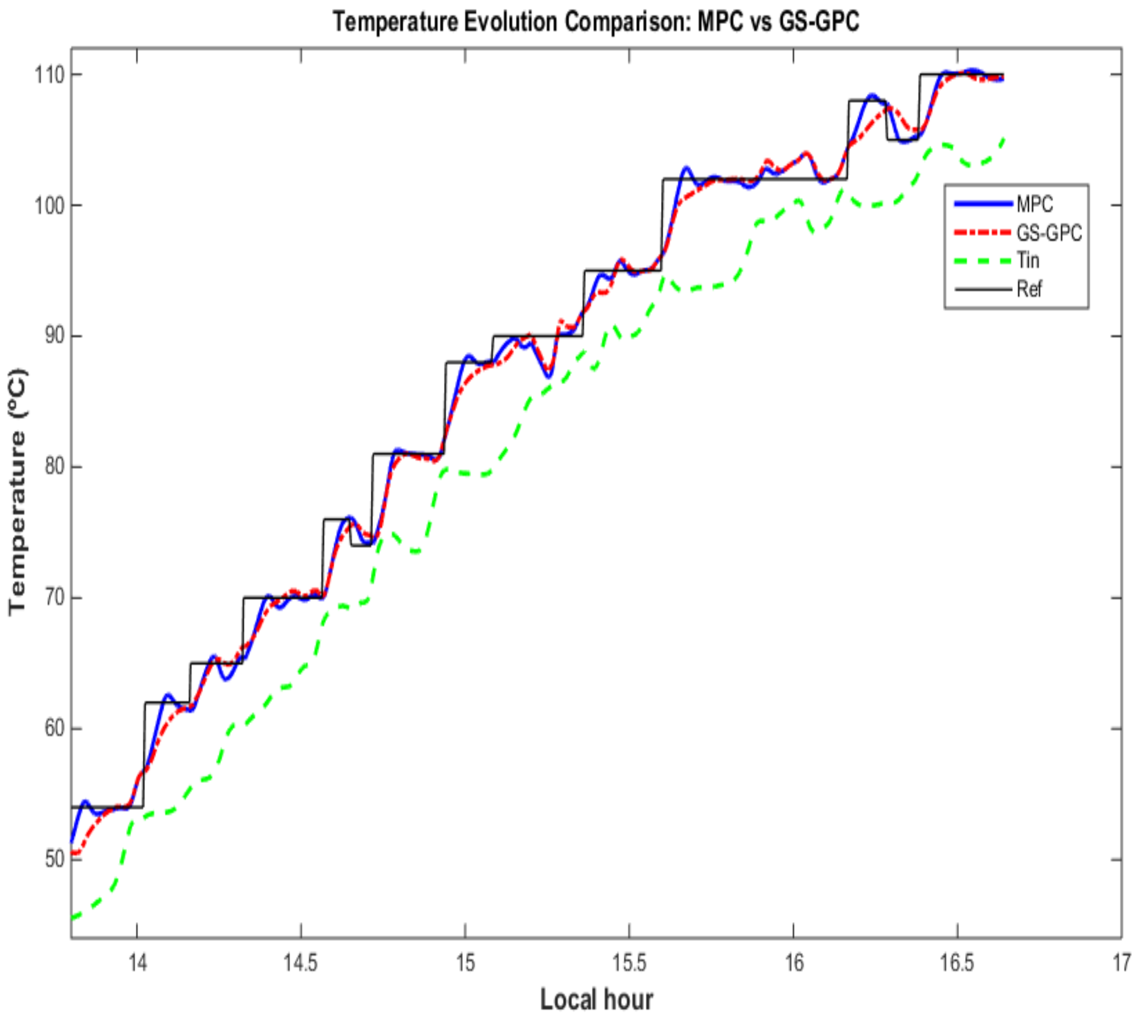
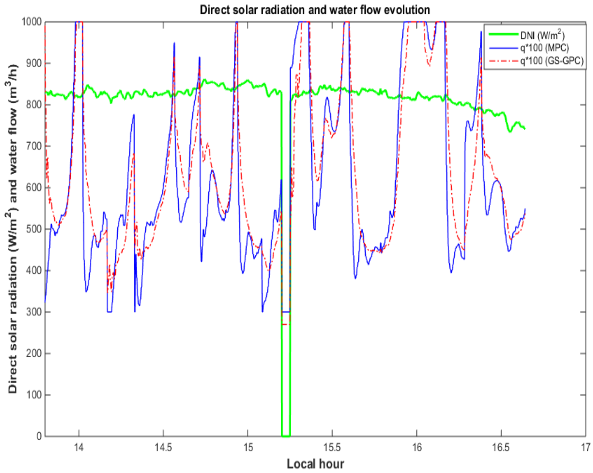
Figure 14 shows the second simulation. The direct solar radiation data corresponds to a clear day with clouds affecting the solar field at 15.2 h (see Figure 15). The data used for this simulation corresponds to the day 6 October 2017.

In this day, the data corresponds to a day where the solar field is working in recirculation mode: the hot water coming out the solar field returns to the input of the solar field after circulating through a pipe. Tracking the references in this mode is not an easy task due to the disturbances in the inlet temperature. The disturbances in the inlet temperature are not easy to reject because they are affected by a delay and this delay depends on the water flow. As can be seen, the MPC tracks faster the temperature references and deals with better the inlet temperature disturbances.

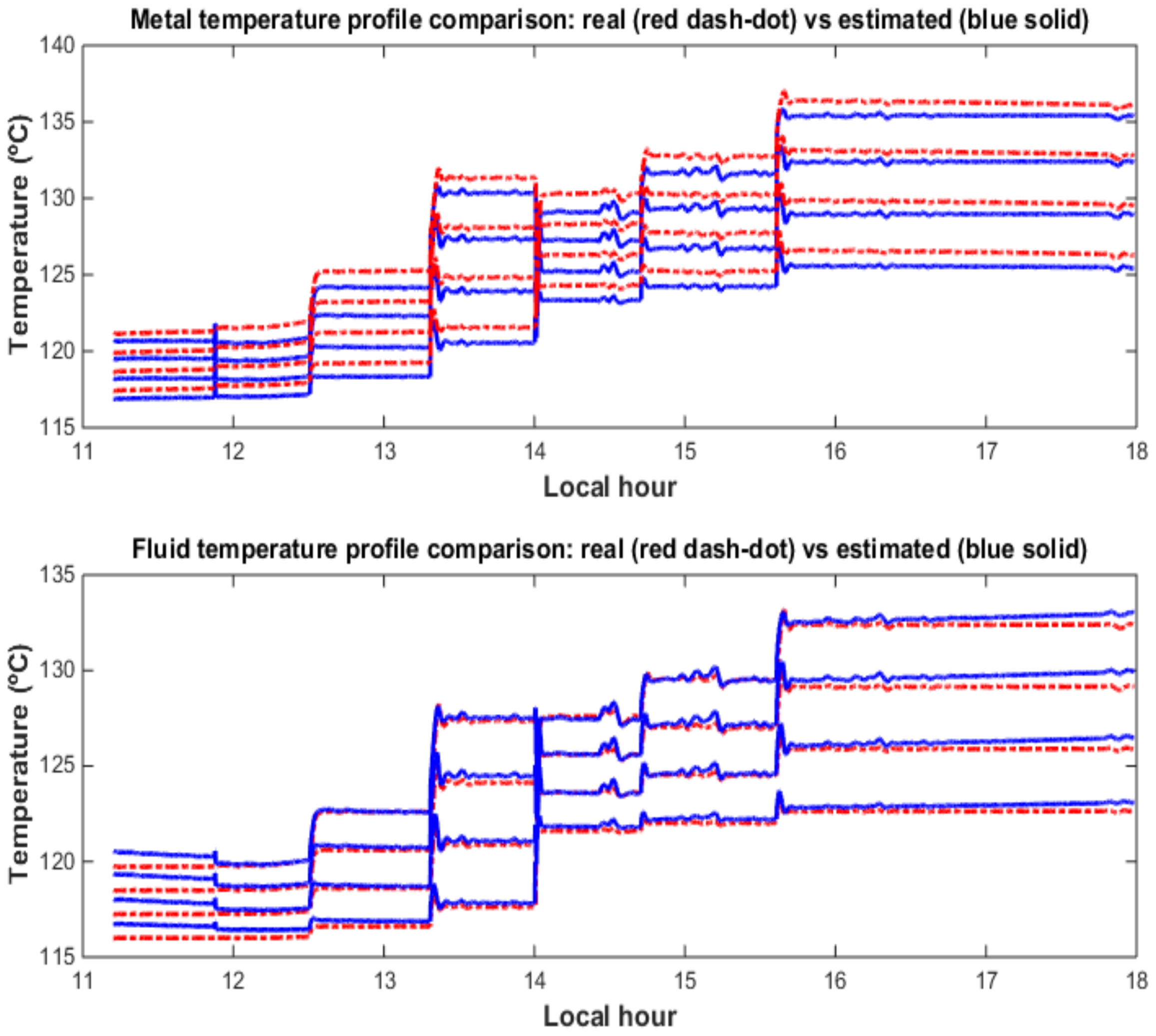
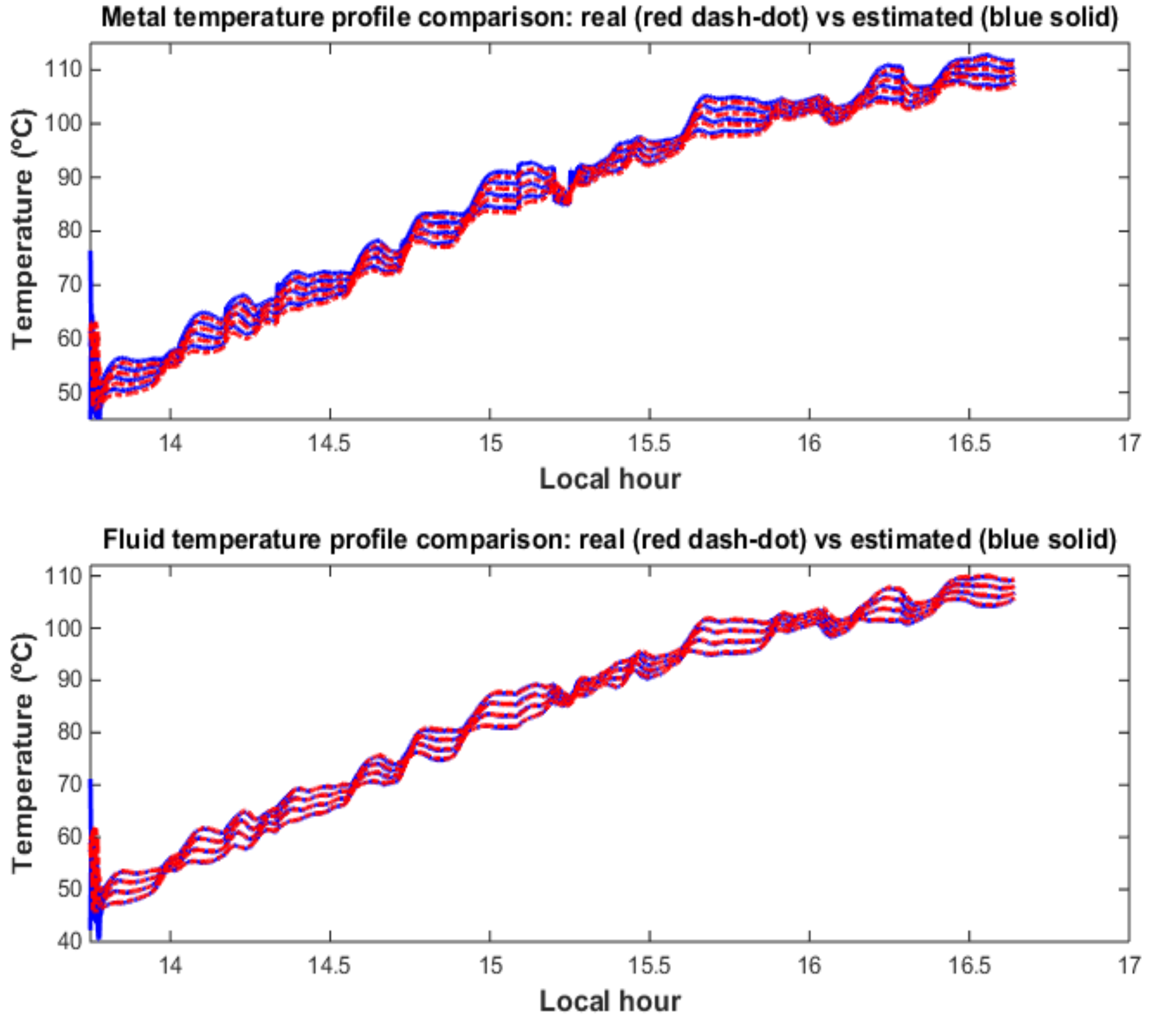
Finally, the comparison between the temperature profiles obtained by the robust Luenberger observer and those provided by the distributed parameter model is plotted in Figure 16. The estimation follows properly the dynamics of the temperature profiles obtained with the distributed parameter model as in the previous simulation, despite the variations in the temperature. As observed in the previous simulation, a steady-state error appears. The maximum error observed is about 0.8 °C.

6.2. Discussion of the Results

In this subsection, a discussion of the obtained simulation results is carried out. The comparison between the two control strategies, the MPC proposed here and the GS-GPC, is analyzed. A control algorithm for a solar power plant should have the following features:

• Fast tracking references: The temperature set-point is usually chosen to maximize the performance of the absorption machine and fulfilling the cooling demand. Thus, tracking as fast as possible the temperature reference is an important issue.
• Disturbance rejection: The controller must be able to minimize the impact of the disturbances affecting the field and tracks the set-point despite them. The main disturbance sources are the direct solar radiation and the inlet temperature.
• Control effort: The controller should not produce a water pump oscillatory response. If the controller is too aggressive with the manipulated variable, the anti-resonance modes may be excited, and the overall performance may be deteriorated as explained in [33].

To compare the performance of the two controllers, two performance indexes are considered. The ITAE (integral of time multiplied by the absolute error) index and the ISE (Integral of Square of the errors) index. The smaller these indexes the better the controller performance. As is shown in the Section 6.1, neither of the controller produces too aggressive responses of the water pumps.

Table 2. Simulation 1: Performance comparison using ITAE and ISE criteria for the comparison between the GS-GPC and the MPC.

ITAE Criterion	GS-GPC	MPC	Improvement MPC over GS-GPC (%)
	3715.2	2612.4	29.69
ISE Criterion	GS-GPC	MPC	Improvement MPC over GS-GPC (%)
	751.95	400.351	46.74

shows the comparison of the ITAE and ISE criteria for both controllers for simulation 1. As can be seen, the MPC control strategy outperforms the GS-GPC control strategy achieving smaller performance indexes. Faster responses are achieved. Table 2 also includes the improvement of the MPC over the GS-GPC in percentage. As shown, the improvement is significative: a 29.69 % in the ITAE criterion and a 46.74 % in the ISE criterion.

Table 3. Simulation 2: Performance comparison using ITAE and ISE criteria for the comparison between the GS-GPC and the MPC.

ITAE Criterion	GS-GPC	MPC	Improvement MPC over GS-GPC (%)
	14117.5	11350.1	19.6
ISE Criterion	GS-GPC	MPC	Improvement MPC over GS-GPC (%)
	4814.5	4106.8	14.17

shows the ITAE and the ISE for the second case. The MPC controller achieves smaller values in the performance criteria. The conclusion obtained is similar to that obtained for the first simulation. In this case, the improvement achieved is smaller but important: a 19.6 % in the ITAE criterion and a 14.7 % in the ISE criterion.

As a final comment, it can be concluded that the MPC obtains a better overall performance. Faster tracking references and better disturbance rejection properties are achieved without a significant increase of the control effort.

6.3. Real Test

In this section, a real test carried out on 22 October 2017 at the real Fresnel collector field is presented. The plant was working in recirculation model, that is, the outlet temperature of the solar field is recirculated through a long pipe and returns to the solar field. In this mode the plant is constantly affected by inlet temperature disturbances. The inlet temperature disturbances are difficult to reject because its associated residence time depends on the water flow [52]. The allowed flow range is confined to 3.7–9 m³/h.

From the beginning to 15 h, the test consisted of a series of changing references which the controller tracks well as seen in Figure 17. The rise times obtained were around 4–6 min. As can be seen, the controller achieves an offset-free tracking.

At 15.2 h the 65 % of the mirrors were defocused for 3 min to simulate a passing cloud. As seen, the controller recovers the temperature after an overshoot of 3.5 °C and steers the outlet temperature to the desired set-point. The effect of the recirculation is seen at 15.4 h, where the oscillation of the outlet temperature produced by the partial defocusing appears in the input of the solar field. The controller rejects the disturbance and tracks the reference properly.

At 15.9 h, the solar field is completely defocused for 4 min. It becomes impossible to track the set-point. When the solar field is again focused, the controller recovers the temperature with small oscillations. The rest of the test consisted of a series of set-points which the controller tracks properly.

7. Conclusions

Advances control strategies can play an important role in improving the efficiency of solar plants. In particular, model predictive control strategies have been applied successfully when controlling solar plants.

In this paper, an incremental offset-free state-space Model Predictive Controller (MPC) is developed for the Fresnel collector field located at the solar cooling plant installed on the roof of the Engineering School of Sevilla. The state-space description uses a robust Luenberger observer for estimating the states which cannot be measured. The effectiveness of the proposed strategy was tested on a nonlinear distributed parameter model of the Fresnel collector field.

The proposed strategy was compared to a GS-GPC, showing a better performance. The estimation of the temperature profile obtained by the robust Luenberger observer was also presented showing a proper state estimation. The estimation is compared to the states obtained by the nonlinear distributed parameter model, because the metal and intermediate fluid measurements are not available at the real Fresnel solar collector field. The maximum error between the estimation and the real metal-fluid temperature profile is about a 1 °C.

The MPC algorithm obtains a better overall performance than the GS-GPC. Faster tracking references and better disturbance rejection properties are achieved without much brisker control efforts. The MPC achieves smaller performance indexes in the two simulations presented.

Furthermore, a real test carried out at the real plant is presented. It shows the good performance obtained with the proposed strategy. Fast reference tracking properties are achieved and rise times of about 4–6 min are attained despite the disturbances affecting the solar field.