1. Introduction
Sub-optimal performance of faulty components in the district heating (DH) systems of today forces the DH system temperatures to be above those theoretically needed to deliver enough heat to the DH customers [
1]. These high temperatures cause heat losses in the system and prevents the utilization of low-grade heat such as industrial excess heat [
2]. Finding the faulty components is key to increasing the energy efficiency of the DH systems.
Previous studies conclude that there are a number of issues in the customers’ installations that cause increased return temperature levels in the DH system [
1,
3,
4,
5,
6,
7,
8]. The customer installation includes the internal heating system of the customer’s building and the substation, which transfers heat from the DH system to the internal heating system.
The internal heating system is most commonly divided into two separate systems: the space heating system and the system for domestic hot water (DHW) preparation. Both of these systems include a number of different components, including control valves, temperature sensors, actuators, pumps, and piping. The space heating system also includes a heat transferring unit in the rooms that are to be heated, e.g., radiators or floor heating, and the DHW system includes faucets where hot water tapping occurs [
9].
The substation design varies depending on different national requirements and/or traditions. In some countries, it is common practice to have a so called direct connection where the DH water is directly used in the internal heating system. In other countries, the indirect connection is the most common solution, where the substation separates the DH system from the customer’s internal heating system. If an indirect connection is used, the heat is transferred to the internal heating system via one or several heat exchangers [
1]. This study focuses on installations with indirect connections, which means that the substations include heat exchanger(s), temperature and flow sensors, control valves, pumps, controller and control system, and a heat meter which delivers data to the DH utility that operates the DH system [
10].
The issues, or faults, in the customer installations may occur in a number of different components and include faults and problems such as fouling of heat exchangers, broken temperature sensors, control valves stuck in an open position, temperature sensors placed on the wrong pipe, DHW circulation connected before the pre-heater, high return temperatures from the customer’s internal heating system, and high set point values in the customer system [
1,
5,
6,
7,
11,
12,
13]. All of these faults may not be seen as an actual fault where something is broken, but they still lead to high return temperatures.
As the DH utilities are now aiming to decrease their overall system temperature, it becomes increasingly important that the vast majority of the faulty installations are detected and corrected. Traditionally, the poorly performing installations have been detected using manual analysis methods [
1]. Due to the vast amount of customer installations in the DH systems, this can be a time-consuming task. Hence, the main focus has been to detect the installations that has the largest impact on the system energy efficiency. This has primarily been done by investigating the excess flow, or overflow, i.e., the difference between the anticipated ideal flow and the actual flow in the installations [
1,
14,
15]. A large overflow indicates that the customer installation is poorly performing, which means that the installations with the largest overflow have been prioritized when conducting the system analysis.
In order to increase the detection rate, the DH utilities can utilize the increasing amount of customer data that has become available during the last few years due to different national legislations and international directives, e.g., the Energy Efficiency Directive adopted by the EU [
16]. This data is collected using the meter device of the substation, and includes supply and return temperature levels, volume flow rate, and the heat amount being used by the customer [
1]. The data is usually used for billing purposes but contains a lot of information about how the customer installations are performing in terms of energy efficiency. This indicates that it is also possible to detect customer installations that are not performing as expected using this data. By investigating the measurements originating from the installations, it is also possible to detect the faults shortly after they have occurred.
Using this customer data, Gadd and Werner used a statistical fault detection method that uses the temperature difference signature of the substation to detect temperature difference faults [
3]. In the study, 140 substations were investigated, out of which 14 were found to be poorly performing. In a subsequent study [
4], Gadd and Werner investigated data from 135 different substations manually. In this study, the results showed that 74% of the substations contained faults, including unsuitable load patterns, low annual average temperature differences, and poor control of the substations. A similar approach was taken by Sandin et al. who used statistical methods, e.g., limit checking and outlier detection, in order to identify poorly performing installations [
8].
A different fault detection approach was presented by Johansson and Wernstedt, using visualization methods to show the operational functionality of individual installations [
17]. In order to aid the subjective visual interpretation, a number of performance metrics describing the relationship between different installation variables were calculated. Xue et al. proposed a fault detection method based on data mining techniques [
18]. The authors investigated data from two installations using cluster analysis and association analysis. The combination of the two methods generated a set of association rules that should be fulfilled in a well performing installation.
Yliniemi et al. presented a method of detecting faults in temperature sensors in a DH substation [
19]. The method was developed in order to detect increasing noise levels in the sensor readings. Zimmerman et al. presented a method capable of detecting faults in pressure sensors and leakages in the DH systems using a Bayesian Network [
20]. Pakanen et al. uses a series of different methods in order to detect faults in the entire customer installation, as well as in three different components of the substation: a control valve, a heat exchanger, and a mud separating device [
21].
The previous studies show that there has been some success in obtaining fault detection methods that can detect the poorly performing customer installations. However, many of the presented methods require an amount of manual handling and/or interpretation. Some of the methods also presume a certain amount of understanding for more advanced computer science and data handling methods. The focus of this study has been to try and eliminate as many manual stages as possible in the fault detection process. The focus has also been to utilize knowledge that is already commonly used in the DH industry to create a fault detection tool that is easy to understand and interpret.
This study presents an automated statistical method for fault detection, which has been developed to detect faults automatically in larger data sets. The method utilizes linear regression and outlier identification, testing the performance of the installation in terms of temperature difference over the installation, the return temperature from the installation, and the heat extracted in the installation.
Furthermore, the method is tested in a case study using real data from a DH system located in Sweden. The data set consists of hourly measurements during one year from 3000 customer installations. The results from the case study show that 43% of the customer installations in the data set are poorly performing.
2. Performance of the Customer Installation
When investigating the performance of the customer installation, a number of different measurements are of interest. One of these is the temperature difference between the primary supply and return temperature in the installation. This temperature difference is often called the cooling, or deltaT (
), of the installation. The cooling depends on both the supply temperature of the DH system, and the return temperature from the customer’s internal heating system. A DH system with higher supply temperature naturally has a larger delta T if the installations are able to cool the DH water well. However, high
’s in a system with high supply temperatures do not necessarily mean that all customer installations are performing well in terms of cooling. When having high supply temperature levels, it is also important to investigate the return temperature levels from the installations to see how well they are actually performing. An installation with high return temperatures from the customer’s internal heating system will not be able achieve a good cooling performance, since the return temperature level from the installation will never fall below the return temperature level in the internal heating system [
1,
3,
10].
Figure 1 displays the cooling pattern as a function of the outdoor temperature for a well performing installation. The grey circles in the figure represent the average cooling in the installation during one day. The red line represents the average cooling in the same installation as a function of the outdoor temperature. The data that the figure is based on originates from a customer located in a city in the south of Sweden where the climate is relatively mild. This explains why
Figure 1 does not display any values for outdoor temperatures below −5 °C. The average supply and return temperatures for the DH system that the installations is located in are 90 °C/49 °C. Hence, the temperature levels of this DH system are quite high and the DH utility is currently working in different ways to obtain lower system temperatures, including performing analysis of the cooling of the customer installations.
As can be seen in the figure, the daily cooling values display a somewhat scattered structure, and the value of
is not necessarily the same for days with the same outdoor temperature. This reflects the fact that the heat demand in the same installation varies from day to day, primarily depending on the varying need for DHW preparation [
22].
As can be seen in the figure, the cooling of this customer installation fluctuates around 50 °C values for outdoor temperatures below 0 °C and then decreases linearly for higher outdoor temperatures. This is visible in the figure where the inclination of the cooling curve (red line in figure) increases for outdoor temperatures above 0 °C. The scattering of the daily cooling values also increases. For temperatures above approximately 15 °C, the need for DH decreases since there is no need for space heating. DH is merely used for DHW preparation at these temperatures, or for industrial processes that require heat during the entire year. This means that the amount of heat that the customer uses is less temperature dependent. Days with an outdoor temperature above 15 °C are in this study called non-heating days. The temperatures where the cooling curve inclination starts to decrease, and the space heating ceases, are called breakpoints. The breakpoints may have other values than in this study, depending on which DH system is being investigated. There may also be more than one breakpoint, depending on the nature of the cooling pattern.
Another measure that may be considered when investigating the customer performance is the heat that is transferred to the building, i.e., the heat that is needed to meet the heat demand of the customer. This heat demand can be calculated according to Equation (
1) [
1]:
where
= volume flow
= density
= specific heat capacity for water (J/(kgC)),
= supply temperature (C),
= return temperature (C).
The heat being transferred is proportional to the volume of water that passes through the substation and the
of the installation. This implies that an increase of one of these parameters would enable a decrease of the other. As it is highly desirable to increase the
, the focus should be on improving the value of
for as many individual customer installations as possible. Furthermore, it is highly desirable to lower the volume flow, since a lower flow rate results in a lower pressure drop in the distribution pipes [
1]. The reduced pressure drop allows for smaller pipe dimensions to be used, which in turn may reduce the building costs of the DH system. A decrease of the pressure drop will also mean that less pump work is needed in the systems [
1,
23].
The decreased volume flow may also be beneficial for the DH customers. Many DH utilities have decided to include a flow price component in their price models for some or all of their customers [
24]. This means that the customers pay for the amount of water mass flow that passes through the customer substation each month, and it is often introduced as an incentive for the customers to improve the performance of their installation [
25].
As mentioned in
Section 1, one of the historically most common methods to identify poorly performing customer installations has been to calculate the overflow, or overconsumption, of DH water for each installation. According to Equation (
1), an installation with a smaller, and hence poorer, value of
will need a larger volume of heat medium to pass through it in order to extract the same amount of energy as an installation with a larger value of
. The extra amount of heat medium is the overflow, which can be calculated using Equation (
2):
where
= actual annual volume
= ideal annual volume
= actual annual energy
= fluid density
= specific heat capacity
= ideal temperature difference (C).
is the ideal temperature difference between the supply and return temperature when the installation is performing ideally. This value may vary depending on what DH system is being investigated, since it depends on the temperature difference between the return and supply temperatures. In this study,
was chosen to be 45
C, in accordance with [
3].
3. Description of Fault Detection Method
3.1. Data Set
The data used in this study was gathered from the business system of a DH utility in Sweden. The time interval was April 2015–March 2016 and it was important to use data from one year since the heat loads of the customer installations are different throughout the year. The data set included data from the 3000 installations that had the largest energy consumption in the system. The installations with the largest energy consumption should be the ones with the largest system impact, and these should be prioritized when performing maintenance work on the DH system in order to improve the system performance. The data set consisted of installations with a wide variety of purposes. The internal heating systems were designed differently for the different buildings depending on purpose of the installation. Hence, no general information was given regarding what specific equipment was used in the space heating and DHW system, e.g., the type of room heaters and if the installations had DHW circulation.
The investigated data set contained values for energy consumption, volume passing through the installation, return temperature and supply temperature for each of the 3000 installations. In addition, the installation ID for the installation where the installation was located, the postal code of the installation, and the outdoor temperatures during the investigated time interval were collected from the business system of the DH utility.
The DH system from which the data was gathered was said to contain weak and non-weak areas. The weak areas were areas known to have a low differential pressure, which means that in these areas it might be harder to deliver heat to the customer installations. This is due to the fact that there has to be a certain amount of differential pressure over the installation for the control valves of the installation to work as they should. If the differential pressure is too low, the installation will not receive the amount of heat that is needed at the installation’s maximum heat load since the control valves will not operate as they should [
10]. The weak areas were well known by the company, and their locations were based on measurements, calculations and simulations of different operation modes of the system. A poorly performing installation had a larger system impact on the DH system if it was located in an area with lower differential pressure than an installation in an area with high differential pressure. Therefore, it was important to be able to distinguish between the installations located in the different areas, and, in this study, the postal code of the area where the installation is located was used to determine if it was located in an area with high differential pressure, or in an area with low differential pressure.
3.2. Data Preprocessing
The data set being investigated in this study originally consisted of hourly values for energy, volume, return temperature and supply temperature for 3000 customer installations in a DH system located in Sweden. Since the hourly values were found to contain some errors which affected the analysis result, the data was first investigated in order to find the errors and handle them according to the nature of the error. After this, the hourly meter readings were converted into daily values as follows: the volume and energy were calculated as the total daily heat use, the supply temperature was calculated as the daily mean value of the measured values, and the return temperature was calculated from Equation (
1). The reason to why the return temperature was calculated in this way was that the measured values of the supply temperature from this DH system were often more reliable than the measured values of the return temperature. This meant that the return temperature values would be more reliable if calculated from Equation (
1). These daily values were then analyzed in order to find the poorly performing installations. A schematic illustration of the data handling process, from the hourly values to the results from the fault detection algorithm, can be seen in
Figure 2, and
Table 1 displays the data included in the data set. The additional data consist of the information about the customers and the investigated time interval that were described in
Section 3.1.
3.3. Choice of Programming Language
The automatic fault detection algorithm developed in this study was developed in the programming language R. R is mainly used for statistical computing and graphics, and include functions for linear and nonlinear modelling, time-series analysis and clustering [
26]. Furthermore, R is an open source program and it is therefore easily accessible to the public.
3.4. Three Signatures
To determine if an installation was poorly performing, three different criteria were used: the cooling performance, the return temperature level, and the energy consumed in the building. The three criteria were used to create three signatures: one cooling signature, one return temperature signature, and one energy signature. The signatures consisted of a reference case, and threshold values which were used for outlier detection.
Since this study primarily focused on identification of installations with poor cooling performance, the cooling and return temperature signatures were considered to be of greater importance than the energy signature. This meant that the installation did not necessarily have outliers according to the energy signature to be considered as a poorly performing installation. The energy signature was mainly developed in order to provide the user of the analysis tool with extra information regarding the installations which were identified as poorly performing.
3.5. Reference Cases
The reference cases of the three signatures were created using data from customers in the investigated data set. This made sure that the reference cases were representative of the system in question. The reference cases contained data from the installations with lowest overflows in the data set.
The reference cases for the cooling and energy signatures were created using piecewise linear regression with one breakpoint for the non-heating days. Piecewise linear regression is typically used to model the relationship between two or more variables in large data set, where it may be hard to find a linear regression model that explains the relationship well for all data. When this is the case, the data set may be divided into smaller segments of data and fit a linear regression model to each of these segments. The segments are divided at the breakpoints, and the combination of the individual regression models is the final piecewise linear regression. The mathematical relationship for a piecewise linear regression model with one breakpoint
H may be described according to Equation (
3) [
27]:
In the equation, , n = 0, 1, 2 are the parameters of the regression model, is the dependent variable being modeled, is the independent variable which is used to model the dependent variable, and is the model error. In the cooling signature, the cooling of the substation was modeled as a function of the outdoor temperature, and in the energy signature the energy consumption was modeled as a function of the outdoor temperature.
The breakpoint for the piecewise linear regression was determined by visually inspecting the data set. As could be seen in
Figure 1, there was a clear change of the inclination of the cooling patterns for lower outdoor temperature levels. This pattern was also visible in the energy consumption patterns. However, when comparing the energy consumption patterns, it was important to keep in mind that different customers consume different amounts of heat. Therefore, it was important to scale the heat consumption so that they were on the same scale. This was done by dividing all heat consumption values for one customer with the maximum heat consumption for that individual customer. After this was done, the breakpoints were determined to assume the values of the outdoor temperature where the inclination of the two patterns changed. This meant that one linear regression modelled the behaviour from the lowest outdoor temperature of the data set to the breakpoint temperature, and the other linear regression modelled the behaviour from the breakpoint temperature to the temperature at which the non-heating days started.
The values for temperatures corresponding to non-heating days were treated separately from the rest of the values. For the cooling signature, the summer days were not considered, since the cooling values for these days only gave information about the size of for DHW preparation in the installations. This may vary greatly from day to day depending on the need for hot water, and hence the analysis of for summer days is not of interest in this study. For the energy signature, the median of the values for summer days was used to create a constant threshold for outlier detection.
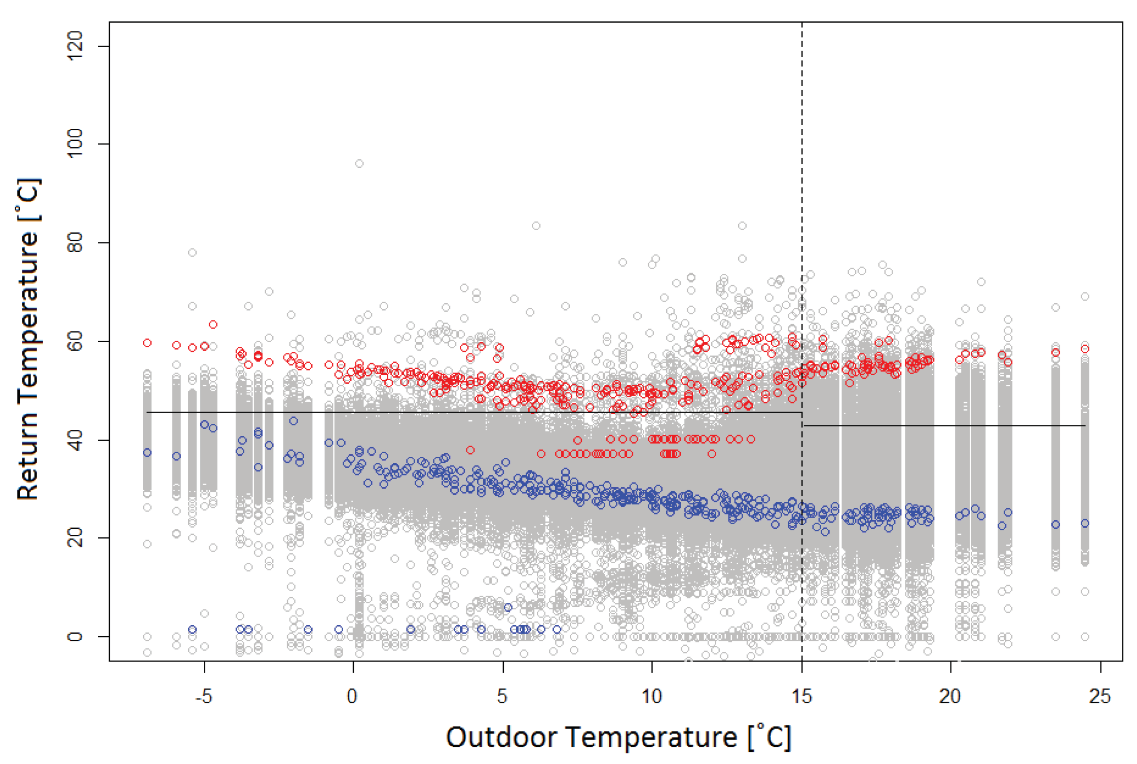
The pattern of the return temperature was completely different from the pattern for the cooling and energy signatures, and linear regression was not a good choice of method for the return temperature reference case. Instead, two constant thresholds were calculated: one for heating days and one for non-heating days. Both of the thresholds were calculated as the mean of the return temperature for the reference case installations.
3.6. Identification of Deviating Values
The performance of the installations not included in the reference cases was investigated to identify deviating behaviours and values, so called outliers. Outliers may be described as values deviating significantly from the expected behaviour of a certain parameter [
28]. The outliers were identified using the mean and the standard deviations of the reference case values. If the distance between the mean and a certain value was larger than three standard deviations for a certain outdoor temperature, the value was considered to be an outlier, in accordance with [
8,
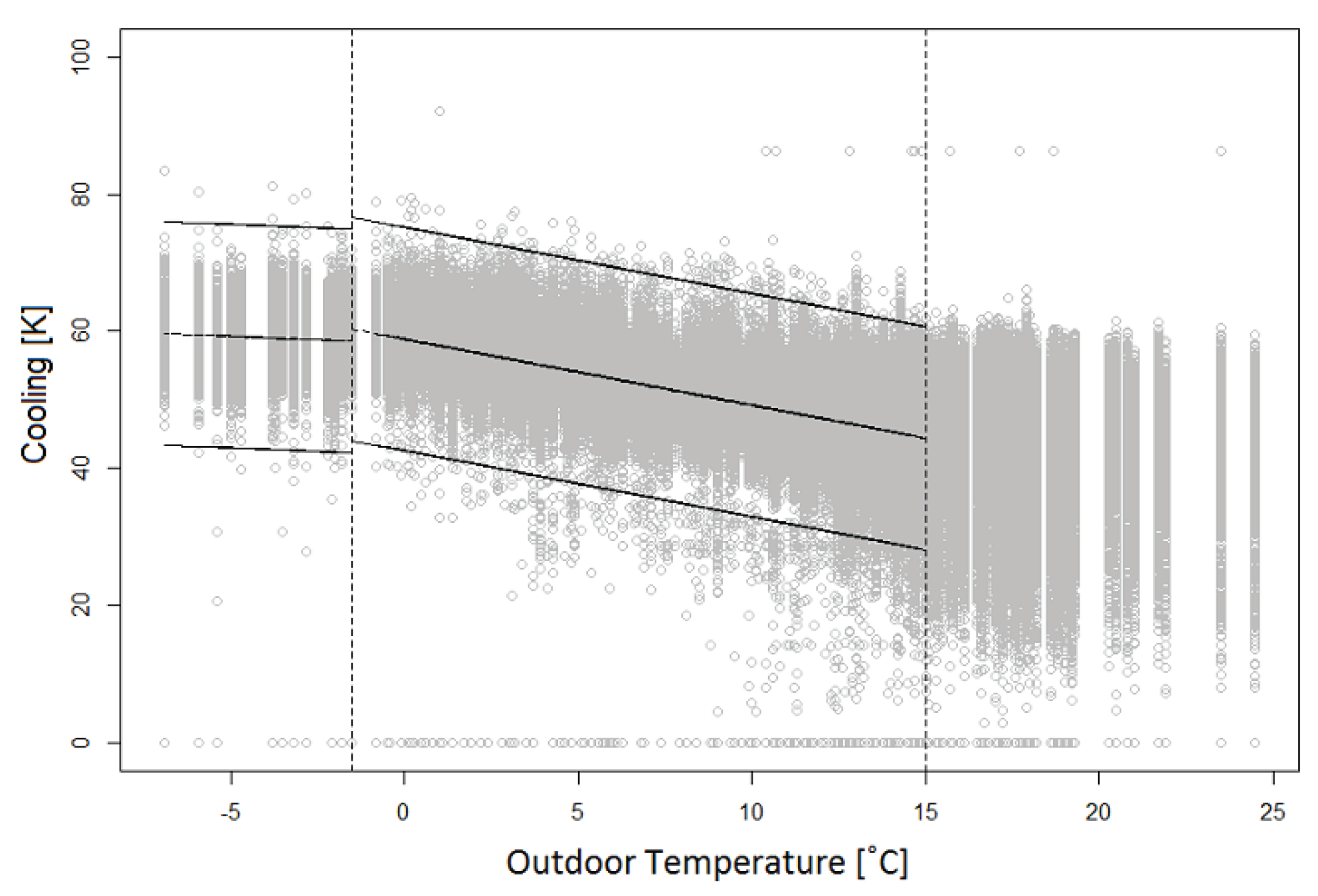
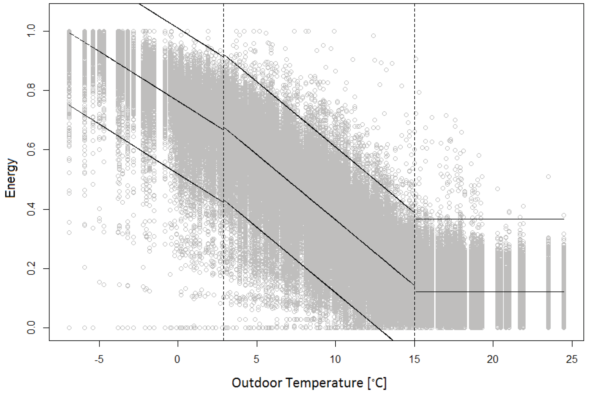
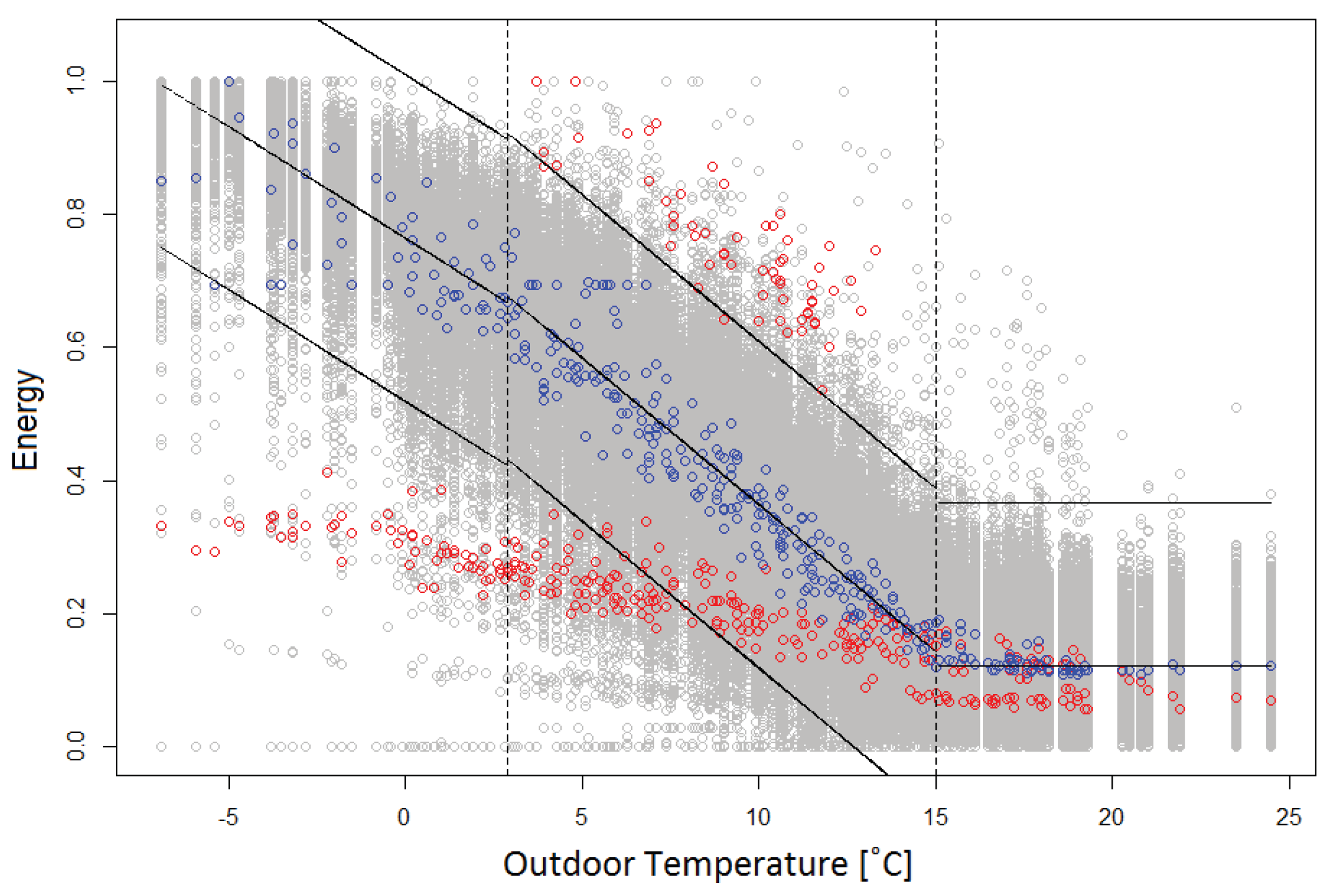
29]. This created thresholds located ±3 standard deviations from the mean. For the cooling and energy signatures, piecewise linear regression was used to model the mean of the reference case and so the thresholds were also linear. For the return temperature signature, the mean was modeled using a constant value, resulting in constant thresholds. The three resulting signatures can be seen in
Figure 3,
Figure 4 and
Figure 5. The reference data set for the return temperature included some measurements that were unreasonable considering the nature of the data. As may be seen in
Figure 4, the return temperature levels sometimes fell below 0
C, which is not plausible in DH systems. These values have appeared when the return temperature was calculated, as described in
Section 3.2. Since the values were calculated in this way, these values were not considered further in the analysis.
4. Description of Fault Detection Algorithm
The algorithm developed in this study consisted of a main function and several different functions which performed different parts of the analysis. The structure of the program can be seen in
Figure 6, and the different functions will be described in detail in the following sections.
4.1. Main Algorithm
The main algorithm, mainAnalysis, loaded and structured the data which was used to perform the analysis. There were also a number of constant parameters that were needed to perform the analysis, e.g., the ideal cooling values. These parameters were determined in mainAnalysis, and can be find in the following bullet list:
The outdoor temperature after which the days were considered to be non-heating days. In this study, the non-heating days occurred for outdoor temperatures higher than 15C.
The ideal cooling value. In this study, was chosen to be 45C.
The specific heat capacity of the heat medium of the system. In this study, the heat medium was water and so = 4185.5 J/(kgC) was used.
The number of breakpoints that should be used for the linear regression, in this study, one breakpoint due to the nature of the heating and cooling patterns (
Figure 1).
The temperatures which should be used as breakpoint values for the linear regression. In this study, two different breakpoints were used: one for the energy signature and one for the cooling signature. The breakpoint for the energy signature was located at 3C, and the breakpoint for the cooling signature was located at −1C.
The threshold values for the return temperature signature, for heating days 45.7C and 42.4C for non-heating days.
The share of installations that should be used in the reference case. In addition, 25% of the substations were used for the reference case in this study.
The number of outliers that were acceptable before the installation was considered to be poorly performing in each signature; in this study, 0 outliers were used.
The number of standard deviations which were used to create the reference case. In this study, three standard deviations were used.
Some of these parameters were system specific, and will have different values depending on which DH system is being investigated. In mainAnalysis, it is also possible to determine if all three signatures should be investigated when running the analysis program. This made it possible to perform analysis of one, two, or three of the signatures, depending on what results the user was interested in.
4.2. Analysis Function
The first subfunction, analysis, was to developed to perform a number of different tasks. The first was to identify which days that were heating days and which were non-heating days, and divide the entire data set in two subsets according to if the data belonged to a heating or a non-heating day. The next task of analysis was to determine what installations to include in the reference case. This was done by ranking the installations according to their overflow, and using the share of installations that was determined in mainAnalysis and had the lowest overflows. The next task of analysis was to determine the number of outliers in each of the three signatures. This was done using three separate functions, dTsign, Trsign and Esign. The function consolidate compiled the results and a created a list of the results. This was returned to analysis, which in turn returned the results to mainAnalysis from which the results were presented to the user.
4.3. Linear Regression
The function
linreg was used to create piecewise linear regression models of the reference case values, and calculate the standard deviation values of the reference cases in the energy and cooling signatures. The breakpoints were placed at the predefined breakpoint value between heating and non-heating days. The parameters of the linear regression models were approximated using the least squares method. The non-heating days were treated differently in the different signatures, and this will be described in further detail in
Section 4.4 and
Section 4.6.
4.4. Cooling Signature
The function dTsign was implemented to create the cooling signature. A linear model of the reference case values, as well as two linear thresholds, were created using linreg. The linear model of the reference case and the linear thresholds constituted the cooling signature of the analysis program. The values of the non-heating days were not included in the cooling signature, and were not considered when investigating the number of outliers in the signature. To find the outliers, dTsign compared the cooling values of each individual installation to the cooling signature and used the linear thresholds to identify the installations which had outliers according to the cooling criterion. The results were compiled in a matrix containing information about the installations and the number of outliers they had according to the signature.
4.5. Return Temperature Signature
The return temperature signature was implemented in a function called Trsign. In the function, two constant thresholds were used to perform the outlier detection: one for the heating days and one for the non-heating days. The thresholds were calculated using the mean value of the return temperatures for the reference case installations. To identify the outliers, the return temperature values of each individual installation were then compared to the constant threshold values and the results were compiled in a matrix.
4.6. Energy Signature
The function
Esign was implemented to identify installations that had outliers in the energy signature. The function was similar to the function
dTsign, described in
Section 4.4, but some additional features were added. As described in
Section 3.5, the different installations consumed different amounts of heat depending on the size of the building and what the building was used for. To enable a comparison of the different installations in the data set, the heat consumption values were first scaled so that they were of the same order of magnitude.
After scaling the values, a piecewise linear regression was created for the energy reference case for the heating days using linreg, and the standard deviation for the reference case substations was calculated. For the non-heating days, the median of the heat consumption values was used to create a constant reference case, and linear thresholds were calculated for the heating days using the standard deviation of the reference case. Esign then identified outliers for both heating and non-heating days and the results were compiled in a matrix.
4.7. Compilation of Results
The functions
dTsign, Trsign and
Esign returned the results matrix to the function
consolidate, which compiled the results from the three signatures to identify the installations that were poorly performing. When running the algorithm with all three signatures, the cooling and return temperature signatures were primarily considered when compiling the results (as described in
Section 3.4. This resulted in the compiled result list possibly containing installations that had no outliers at all according to the energy signature. If only two signature functions have delivered result lists, the
consolidate function created the final result list from the available results. If the algorithm only investigated the installations using one of the signatures,
consolidate used the results matrix from that signature function. When more than one signature was used,
consolidate compared the installation IDs in the result lists from the different signature functions. If the installation appeared in more than one list, it was included in the final result list with poorly performing installations.
Due to the nature of the DH system that the data originated from, two result lists were created. One contained installations located in the weak areas of the system, and one contained installations located in the non-weak areas of the system. The installations in the list were ranked according to the overflow of the installations. The list contained the installation IDs, the number of outliers for each of the three signatures, if the installation was located in a weak or non-weak area, and the overflow of the installations. The compiled list was then returned to the analysis function and presented to the user in the mainAnalysis function.
6. Analysis and Discussion
The results from the customer installations analysis algorithm state that 43% of the total amount of the investigated installations are performing poorly. This indicates that it is possible to make large improvements in the overall DH system performance, if the poorly performing installations are fixed. In the future DH systems, this will be necessary to maintain the low temperatures that enable the use of other and more efficient heat sources. Therefore, some sort of automatic installation analysis method will most likely be a necessity in all future DH systems.
Even though the entire system was not investigated, the number of investigated installations is larger than those of previous studies. The use of the analysis tool could easily be extended to an entire DH system by using larger data sets. The results from this study clearly show that it is possible to identify poorly performing DH customer installations in large data sets, without having to perform the time-consuming manual analysis that a lot of DH companies are relying on today.
Regarding the results in
Table 2 and
Table 3, it is clear that the installations presented all have a large overflow. Two of the installations in
Table 3 have overflow values over 100,000 m
, which means that a very large additional amount of DH water is passing through the installation each year. These installations are located in the non-weak areas of the system and so have a smaller impact on the system performance than they would in a weak area. However, the large overflows are a clear indication that there is room for significant improvements of the system efficiency if action is taken to fix the installations in question. From
Table 2, it is clear that there are a number of installations located in weak areas that have a very large overflow per year. Due to the increased amount of flow that passes through the installation to meet the heat demand of the customer, the pressure drop over the installation will increase. This means that the areas where it is already hard to maintain the differential pressure levels will be even more affected by installations that are not working as they should, giving further incentives that the installations in the weak areas should be fixed as soon as possible.
The analysis method used in this study is based on customer data and patterns that are very familiar to the DH utilities. This is a big advantage since the method is easier to understand compared to other, more advanced computer science methods. When developing a new analysis method, it is important to keep the end user in mind and, by utilizing what is already very familiar within the industry, it will be easier to also implement the developed method and the understanding for it would be more intuitive. For example, figures similar to
Figure 7,
Figure 8 and
Figure 9 give a nice overview of the performance of the installations using patterns that are very familiar to people in the DH industry, and could be used to present the results to the end user of the algorithm.
The share of poorly performing installations that was identified in this study deviates from the shares that have been identified in previous studies. For example, Gadd and Werner show that 74% were poorly performing [
4]. One of the reasons to why this is the case might be that the definition of what is considered to be a well performing installation is different in the different studies. This means that the reference case will have different properties, depending on the definition of a well performing installation. This will have a large impact on the result, since the reference case values decide the threshold lines. If the reference case contained less installations, it might be that the standard deviation of the reference case values is smaller, hence creating a narrower reference case signature. A narrower signature results in more installations being identified as poorly performing.
Another reason for the deviation might be that a larger data set includes more installations of different purposes, which uses heat differently during the day. The different building types have heating patterns that might differ largely from each other due to which type of heating control system is used in the buildings. Some types of buildings have a very wide heat pattern, e.g., office buildings, since their daily average heat demand is significantly lower during days when nobody is present in the premises. This means that an office building can have a wide range of different values for one single outdoor temperature, and this causes a wider heat pattern. If the reference case includes installations with these wide heat patterns, they may contribute to the reference case being wider than it would be if only installations with a narrow heat pattern were to be included. Since the data set in this study contains a larger number of installations compared to the previous studies, it is likely that the reference case in this study contains a larger variation of buildings. This indicates that the thresholds in the reference cases of this study will be more allowing than for a smaller data set, and therefore less values in the data set will be identified as outliers. However, the number of installations that was identified as poorly performing in this study is still very high. This clearly indicates how important it is to be able to identify the poorly performing installations in a quick and efficient way in order to be able to improve the overall performance of the DH systems.
In this study, the ideal value for was chosen to be 45 C, in accordance with the results from other studies. However, this is a parameter which is very dependent on the system that is being investigated since the temperatures of the system might not allow that a value of 45 C is obtained. If the temperature difference between the supply and return temperature is, e.g., 30 C, then it will not be possible to obtain the ideal used in this study. It might also be that a DH system has very high supply temperatures, which means that it is “easier” to obtain high ’s. This indicates that, in some systems, the ideal in this study might be small in a system with high supply temperature. Therefore, it is of great interest to find another way to determine what value should be used as the ideal if this analysis program is to be used in other DH systems.
When considering the fault detection method used in this study, there are some variables and approaches that could be done differently. One example is the value of the ideal as described above, and another is how the reference case installations were chosen. In this study, the reference case was decided based on the overflow of the installations. Hence, the installations with the lowest overflow were included in the reference case. There might be other ways to determine the reference case installations, e.g., by choosing the installations with the lowest return temperatures. It might also be interesting to rank the poorly performing installations differently. In this study, they were ranked according to their overflows. Other possibilities would be to rank them according to the number of outliers in each signature, or to rank them according to the total number of outliers in all signatures. It would also be possible to choose the breakpoint of the piecewise linear regression differently. In this study, one breakpoint was used and the value of this was determined by visual inspection of the customer data. The choice of breakpoints could have been further improved by using statistical methods.


