Demand-Side Management with a State Space Consideration


Department of Electrical and Computer Engineering, United States Naval Academy, Annapolis, MD 21402, USA
Energies 2018, 11(9), 2444; https://doi.org/10.3390/en11092444
Submission received: 6 August 2018
/
Revised: 3 September 2018
/
Accepted: 13 September 2018
/
Published: 14 September 2018
Abstract
:Power networks are gateways to transfer power from generators to end-users. Often, it is assumed that the transfer occurs freely without any limiting factors. However, power flows over a network can be limited by predetermined limits that may come from physical reasons, such as line capacity or Kirchhoff’s laws. When flow is constrained by these limits, this is called congestion, which reduces the energy efficiency and splits the price for electricity across the congested lines. One promising, cost-effective way to relieve the impact of the congestion is demand-side management (DSM). However, it is unclear how much DSM can impact congestion and where it can control the demand. This paper proposes a new DSM mechanism based on locational willingness-to-pay (WTP) centered around income statistics; utilizes a state-space tool to determine the possibility to alter prices by DSM; and formulates a convex optimization problem to decide the DSM. The proposed methodology is tested on IEEE (Institute of Electrical and Electronics Engineers) systems with two commonly used objectives: cost minimization and social welfare maximization.
1. Introduction
Demand for electric power keeps increasing in modern society with advancements in technology and the rise in commercialization. The increase shows geographic variation (e.g., demand in urban areas grows more rapidly than that in rural areas). Since the construction of electric power systems, such as generators and grid systems, is highly limited, the locational discrepancy between demand and supply raises concerns about successfully accommodating such a rapid increase. When there is insufficient energy to meet the demands locally, the discrepancy between demand and generation must be fulfilled by an external system through the transmission grids. There is a limit to bringing electric power over the grids; attempting to operate a system beyond its rated capacity is likely to result in line faults and electrical fires. Congestion is another issue that crops up, referring to when the grid’s limit is met, requiring a tuning of the system to increase the capacity, adding new transmission infrastructure, or decreasing end-user demand for electricity [1]. However, in modern society, the opposition by residents to a proposed development in their local area makes it difficult to expand power systems.
In a restructured electric power system, the electricity market is a commodity for trade through bids to buy and through offers to sell, where supply and demand principles are used to set the prices [2]. These bids from consumers form the basis of demand-side participation. Demand-side management (DSM) was introduced publicly by the Electric Power Research Institute (EPRI) in the 1980s [3]. DSM now covers a broader functionality of planning, implementing, and monitoring activities of electric utilities, which are designed to encourage consumers to modify their levels and patterns of electricity use [4]. Recent studies show that the public prefers renewably generated electricity [5] and that it is willing to a pay premium for it [6]. Various types of demand measures have been used over the years, including energy-efficient devices, demand-response incentives that promote intentional energy-use modification on the consumer side, dynamic demands to balance the load peaks, and distributed energy resources. While collecting real-time data on the measures will become more feasible as the Internet of Things evolves, and the utilization of the real-time willingness-to-pay (WTP) is most relevant for demand-side bidding, the real-time WTP is not yet readily available. Depending on the type of demand, however, some demand-side manipulation can be implemented [7]. For example, elastic demand can be bid for and it is acceptable for some demand to be not served [7]. We propose a simple model to utilize local salary information to derive the bids. The simulation environments are as follows: (1) generators submit their offers to the market and the central dispatcher clears the market for finding generation dispatch and prices; and (2) load aggregators intervene to adjust demand to improve the dispatch (either increasing social welfare or reducing system cost). The results are compared to those of a clearing market with the demand-side’s bidding directly to the market. The novelty of this paper is in the integration of DSM using publicly available data related to the WTP and income statistics. In addition, it proposes the development of a new methodology for an engineering tool to enhance the market performance and for socio-economic application in the DSM.
2. Modeling of Willingness-to-Pay Curves
2.1. Modeling Willingness-to-Pay Curves
For the sake of modeling simplicity and data accessibility, we propose a simple WTP curve based on publicly available household salary data [8]. Figure 1 shows the cumulative salary distribution of the three cities in blue (Buffalo), green (Rochester), and red (New York City), respectively.
We assume that the salary x follows normal distribution f(x) at a given mean μ and standard deviation σ, as follows:
The cumulative normal distribution F(x) is:
where erfc is the complementary error function.
Data fitting to the salary data yields the mean μ and standard deviation σ (see Table 1 for the values and Figure 1 for the fitting results). In addition to the salary data, Table 1 also lists the demographic data from [9].
It is suggested that there are two types of demand: price-based and must-serve [7]. For their modeling, interruptible load contracting (ILC) denotes the number of times the demand does not need to be met within a given contract period. In this case, the demand is assumed to be price-based and the distributor has not used all its ILC. Based on Fermi–Dirac statistics [10], which can fulfill individual demands differently based on priority, the optimal bidding function for price-based demand derived from [7] is used to calculate the WTP bidding curve:
where p is the WTP in $/MWh; pmax is the maximum WTP in $/MWh; pr is the readily acceptable WTP in $/MWh; d is the local demand in MW; df is the forecast demand in MW at the location; and fr is the freedom factor. We derive this WTP curve p(d) with an estimate of fr and pr from the cumulative salary curve as follows: . The WTP curves are illustrated in Figure 2. For this figure, the proportionality constants are .
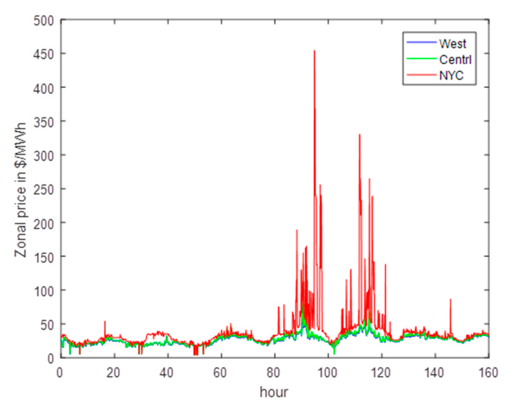
Three zonal prices during the last week of July 2018 [11] are illustrated in Figure 3: Buffalo, Rochester, and New York City (NYC) belong to west, central, and NYC, respectively. As shown in the figure, the price in NYC is the highest while those of central and west New York are similar, the WTP shifts to the right as the average salary increases, and the curve becomes less steep as the standard deviation increases. Given the dispatch at the ith location,, where ρ is the price of electricity and the superscript 0 refers to an initial value, one can linearize the WTP curve near the dispatch, such as: . Therefore, the change in the demand surplus k (the area under the WTP curve: cost to purchase the electricity) is:
where Lg and Ld are matrices to identify the locations of generators and demands, respectively. Note that (4) is a quadratic function with the local demand di, and that the second term vanishes if the demand control does not change the electricity price.
2.2. Direct Current (DC) Optimal Power Flow
Optimal power flow finds an operation point for clearing markets for the operation of electric power systems. For the sake of reducing the complexity in numerical computation, a linearized model is generally used; a direct current optimal power flow (DC OPF) problem with generation g and demand d:
where k and h are demand surplus and generation cost, respectively; Bbus and Bbr are the nodal and the branch admittance matrices, respectively, of which the corresponding column to the reference bus is eliminated; fmax, gmin, and gmax are the flow limits, the generation minimum outputs, and the generation maximum output, respectively; and θ is the voltage angles at the non-reference buses. The DC OPF problem is solved with the MATPOWER software package [12].
2.3. State Space
The solution of (5) includes the price for electricity—known as locational marginal pricing (LMP)—which is the shadow price of locational power balancing. Therefore, the LMP indicates the value of electricity at the corresponding location. In the DC OPF problem, LMPs are heavily dependent on congestion. With the aim of modeling different LMPs when the demand is altered, a state space is determined. Let be the set of possible state vectors. Given a realization of meter data z, the control center obtains the state estimate . From , one obtains the estimated congestion pattern (also a function of z). From the estimated congestion pattern , a real-time price is obtained. Since the state estimate is taken as a sufficient statistic, we can drop the original data z. As a result, each x ∈ X is associated with a congestion pattern C; thus, the real-time price is ρ(x). We define π(C) as the region of xs, which gives the congestion pattern as C. The state space is generated using multi-parametric programming, which aims to obtain the optimal solution as an explicit function of the parameters. It is based on the sensitivity analysis theory [13,14]. Sensitivity analysis provides solutions near the nominal value, whereas parametric programming provides a complete map of the optimal solution in the space of the varying parameters [15].
Using a quadratic cost curve with 0.5qc (quadratic cost coefficient) and lc (linear cost coefficient), the DC OPF problem becomes:
The Taylor Series at the operation point yields:
where n, σ, and ξ are the number of constraints, the corresponding shadow prices, and the slack variables, respectively. The solution satisfies the Karush–Kuhn–Tucker (KKT) conditions as follows:
This is where parametric programming detaches from the sensitivity analysis theory. The state space of d where this solution remains optimal is defined as the critical region CR, which can be obtained by using feasibility and optimality conditions. Feasibility is ensured by substituting g into the inactive inequalities given in (6), whereas the optimality condition is given by , where corresponds to the vector of active inequalities. As a result, a polyhedral region is formed by the set of parametric constraints represented by:
where correspond to the inactive inequalities and CRIG represents a set of linear inequalities defining an initial given region. Redundant inequalities are removed, and a compact representation is found by , where Δ is an operator that removes redundant constraints. Once it has been defined for a solution, the next step is to define the rest of the region . Another set of parametric solutions in each of these regions is then obtained, and corresponding CRs are obtained. The algorithm terminates when there are no more regions to be explored [16].
2.4. Improving the Objective Function with Demand-Side Management
The minimization of a quadratic generation cost [17] is the most widely used objective function in operating power systems, i.e., k(d) = Nd >> 0, where N is the value of an elementary demand. If a certain fraction of the demand control is predefined using the state space, one finds the original and the new dispatch on the state space. Suppose 10% of load shedding is allowed, then is imposed. Only state spaces within 0.1 distance of the Nd-dimensional -sphere are reachable from the current state spce. Once the state spaces are identified, the set of binding constraints is selected (Mbinding and Nbinding in (8) are found). Correspondingly, the generation g is computed in terms of the change in demand d–d0 using (8). The system cost is
In the case of maximizing the social welfare, i.e., , where the quantity in the square braket is the suppliers’ surplus, the sum of the suppliers’ surplus and the consumers’ surpluses is:
Note that pinj is the power injection vector. For the DC OPF problem, the price is expressed in terms of the shadow price to the system-wide power balance equation (), and the shadow prices σ of binding line flow limits. For example,, where Hc is the shift factor corresponding to the congested lines: . (10) and (11) are generalized as follows:
and is symmetric positive semi-definite for a positive qc. Eigenvalue decomposition reveals the eigenvector and eigenvalue pair. Correspondingly, if is a full rank matrix, one can formulate an optimization problem:
where δ is a predefined limit of DSM. Using the inequality relationship between 2-norm and -norm (i.e., ), a least-square minimization over a sphere is formulated:
Because the feasible region of (13) is a subset of that of (12), the solution to (13) is guaranteed to be feasible for the original problem (12). There is an efficient algorithm to analytically solve (13) with a singular value decomposition of a rank-r matrix A, [18].
- If , a scalar value of λ* is easily identified by a divide-and-conquer approach to satisfy , where . The solution x is:where ej is the jth column vector in an identity matrix.
- Otherwise,If is a rank-deficient matrix, a minimization problem is formulated:(16) is a quadratic programming.
3. Simulation Results
State-Space Representation
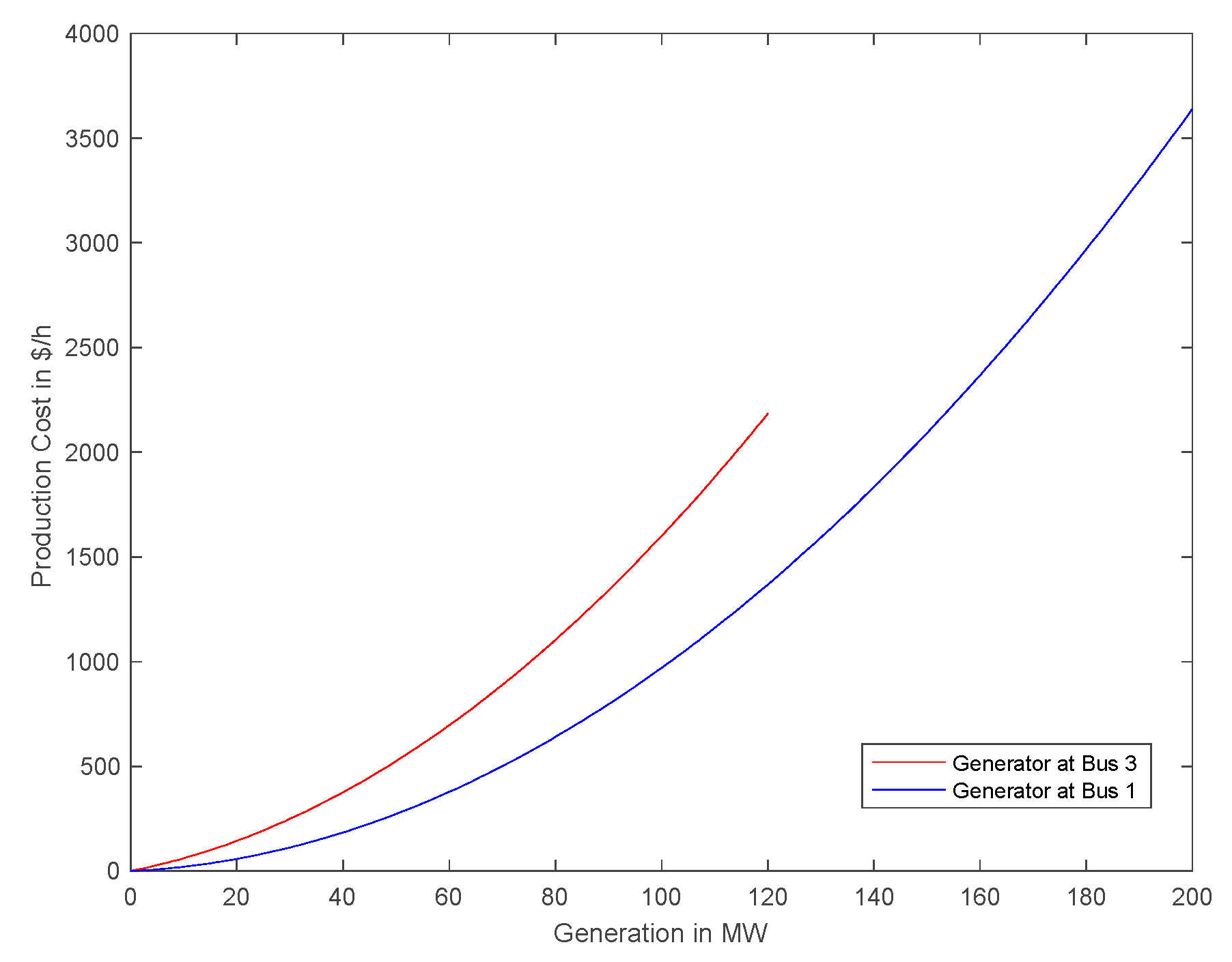
The IEEE 3-bus system is defined in the above formulation and the state space is determined using the Parametric Optimization Toolbox [19]. The optimization problem is solved and converted into a state space as shown in Figure 4. The generator at Bus 1 is a base unit and Bus 3 is a peaking unit (i.e., the one at Bus 1 has a lower generation cost than that at Bus 3). Figure 5 illustrates the quadratic generation costs. The marginal cost of the peaking unit increases as its generation output increases up to $31.4/MWh at its maximum generation of 120 MW. The base unit will have the same marginal cost ($31.4/MWh) when its generation output is 177.65 MW.
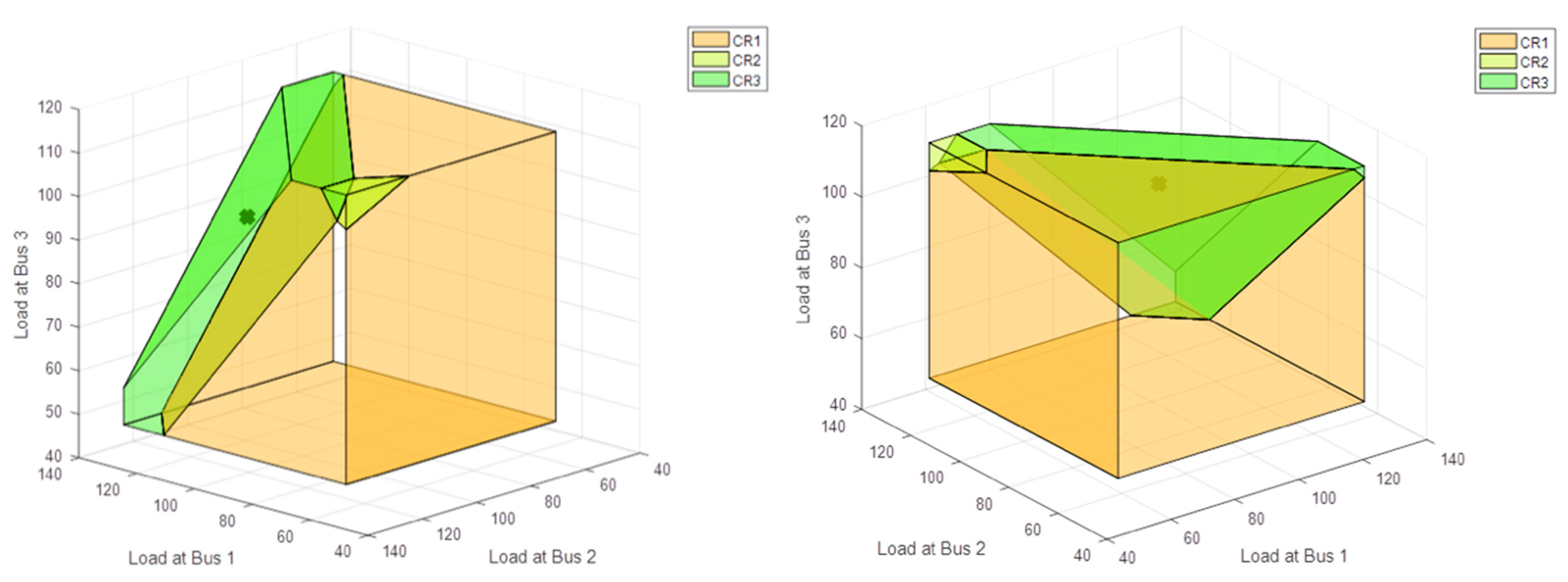
The line connecting Bus 1 and Bus 2 has a limited capability for power flow, and the generators have generation constraints. As a result, there are three critical regions: CR1: the base unit fulfills all the demands where the sum is less than the maximum generation capacity of a generator; CR2: the peaking unit is necessary to serve the demands due to the flow limit between Bus 2 and Bus 3; and CR3: the peaking unit also serves demand because the demands exceed the maximum capacity of a generator. Figure 6 visualizes the critical regions. The x-mark—110 MW, 95 MW, and 110 MW—indicates the current demands that is in CR3, and the generation cost is $5650.13/h. The critical regions are shown in different colors separated by hyperplanes corresponding to the constraints. The equations to describe the boundaries between CR1 and CR3 and between CR2 and CR3 are: and .
The distances between the current dispatch (x-mark) and the boundaries are 10.02 MW (CR1–CR3 boundary) and 47.76 MW (CR2–CR3 boundary), respectively. In our study, we impose a condition that the DSM is allowed up to 10%. While 10.02 MW is in the range of 10% reduction of total demand, 47.76 MW is not. Furthermore, CR2 is a more expansive alternative as it requires the peaking unit and line congestion. Therefore, the DSM does not consider the change in the critical region toward CR2. The transition to CR1 is possible in the demand reduction in at least 10.02 MW in the normal direction of the boundary between CR1–CR3 (0.5774; 0.5774; 0.5774). As a result, the demand should decrease 5.785 MW at all buses. Since this change is feasible in the scope of 10% reduction of the current demand, we will consider the DSM in that direction.
In CR1, the generation dispatch is constrained neither by generation capacity nor by congestion. The new dispatch should satisfy , where the bottom equation is that the marginal generation costs of both generators must be the same. This leads to , where and . Solving the optimization yields and the generation cost is $4376.4/h. In summary, 10% reduction in demand (−31.5 MW) decreases the system cost by $1273.73/h (approximately 23% reduction in the system cost).
It is noteworthy that, in the above computation, the nodal values of demand are not considered. Therefore, within CR1, demands uniformly decrease at all locations. Suppose the WTP curves are given at each location (e.g., Bus 1 is Rochester, Bus 2 is New York City, and Bus 3 is Buffalo). Since there is no congestion, price separation over geographic areas will not occur (i.e., pRoc = pBuf = pNYC). However, the sensitivities of price with respect to demand are different. For example, . For those three cities, the values for Rochester, for New York City, and for Buffalo are −5.5741, −6.3071, and −5.3985, respectively. In CR1, by assuming the price is near $31.4/MWh and , at Rochester, at New York City, and at Buffalo are −$169.45/MW2h, −$191.45/MW2h, and −$164.12/MW2h, respectively. The values indicate how much the price should decrease to attract demand response. Actual demand response in New York shows that Western New York, including Buffalo, has a very active demand-response program [20]: it’s the second-largest demand-response program after New York City (approximately 75%). Given that the demand in New York City is much higher than in Buffalo, the relative demand response is remarkable in Buffalo. The solution to the social welfare maximization shown in Equations (14) and (15) is to satisfy the demands (100 MW, 86.5 MW, 100 MW). Since the value of the electricity in New York City is higher than the other two cities, it is reasonable to reduce the demand at New York City at a lesser degree. Even though this solution results in a higher generation cost than the 10% uniform reduction in demand (the solution to the cost minimization problem), it does not significantly reduce the demand surplus significantly. For a comparison purpose, we applied a new market rule where demand-side bids were allowed and the market was cleared either for maximizing social welfare with the WTP curves or for minimizing the system costs. The results are very close in terms of optimal reduction of demand and of the objective function value within 1%. This result is promising in that the performance of our distributed decision by demand aggregators is approximately the same as that of the central decision with WTP curves in dispatch.
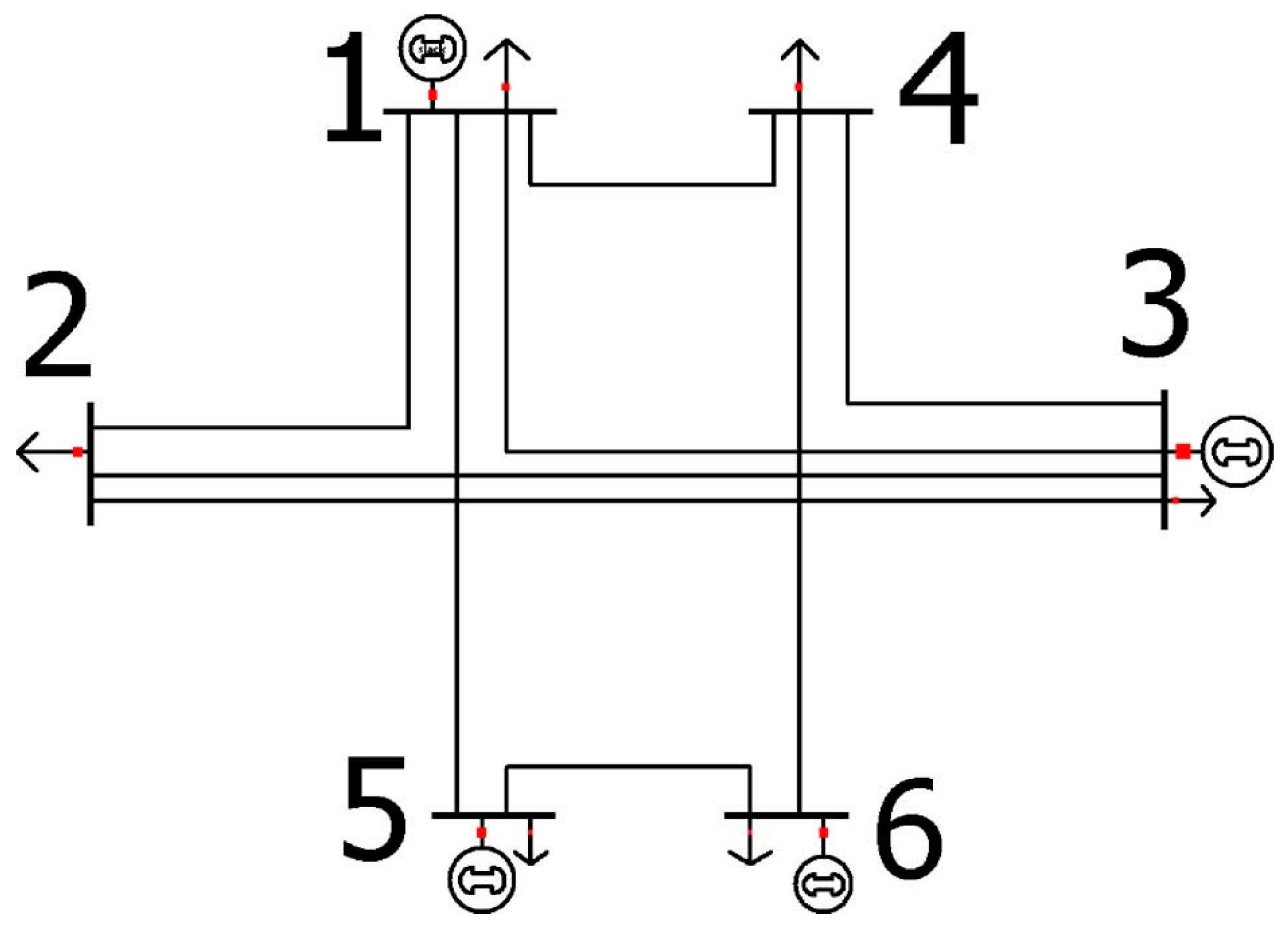
To apply the proposed model for a larger system, the IEEE 30-bus system is considered. A network reduction method has been suggested that preserves the congestion pattern of the original network [21,22]. The IEEE 30-bus system is reduced into a 6-bus system by grouping (see Figure 7). Because the demands are located at all six buses, it is not possible to visually present the state space. However, from the state space, one finds that the current dispatch is within CR1 that has two congested lines: Bus 2–3 (σ2→3 = $130.72/MWh). By computing the distances between the current dispatch and all the CR boundaries, we found that 10% of demand reduction will not cross any CR boundaries. Therefore, we concluded that the demand reduction will occur only within CR1, which yields a price that is approximately the same. Equation (8) gives:
This yields: and the change in the system cost is . Since the initial generation cost is fixed, the minimization of the change in the generation cost is equivalent to that of the generation cost. Eigenvalue decomposition finds since there are only four nonzero elements in while demands are distributed in six locations. The eigenvector matrix is a rank-deficient matrix, and therefore one constructs (16) as quadratic programming to minimize the change in the system cost such that: . Its solution is . The cost reduction is $701.3/h (approximately 17% of the original system cost of $4082/h) by reducing 16.48 MW (uniform 10% demand reduction over the entire system). Figure 8 illustrates the contour of the generation cost with the change in demands at Buses 1 and 4 while fixing all the demands at the other locations. The control of demand at Bus 4 yields only marginal changes in the system cost, whereas it yields a significant impact at Bus 1. As shown in the optimal demand reduction vector Δd, the demand reduction at Bus 1 is significantly more efficient than that at Bus 4.
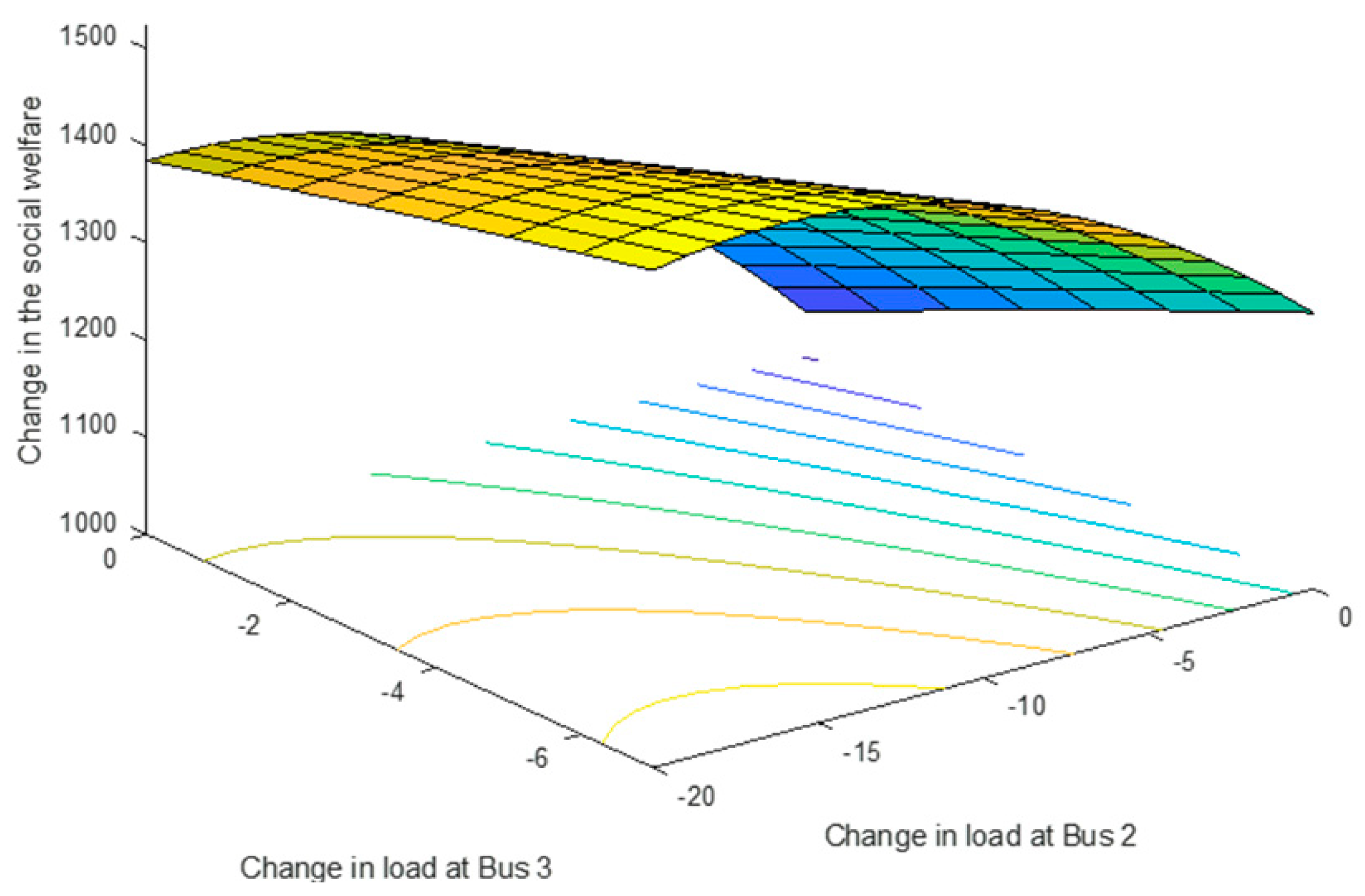
Different from the cost minimization problem, is a full-rank matrix for maximizing social welfare. Since the reduction of demands does not change the critical regions, the set of binding constraints stays the same. In the same critical region, the adjustments in demand are made in a way that the flow over the congested line does not change (neither increases since the flow is at maximum, nor decreases as the decrease would negatively affect the objective function). Therefore, . For the sake of simplicity, we assume that the standard deviation and mean of household salary are approximately the same (see Table 1), and that p << pmax based on the price range from the simulation of [$24.7/MWh, $54.1/MWh] where pmax = $1,000/MWh. Therefore, . This price sensitivity with respect to demand makes a full-rank matrix, and the solution to (13) is identified using (14). The solution to this least-square problem over a sphere is: . In comparison to the solution for reducing the system cost, the demand reduction occurs to the same degree, save for Bus 1. As we increase the value for δ, the reduction occurs at a different level. For example, at δ = 0.3, the reductions at all the locations are different. The reduction difference increases as the price of electricity increases, which is intuitively correct since the value of electricity indicates the degree to give up the demand fulfilled. Different from the cost minimization problem, the demand control has a certain optimum point. This can be explained in the following plot. Using the values from Table 1, the contour of the social welfare for the IEEE 3-bus system is illustrated in Figure 9. Social welfare increases when controlling demands at both Bus 2 and 3 are initially at (0, 0). While that is true for Bus 3 over the entire 10% demand control, the social welfare starts to decrease beyond a certain point at Bus 2. This indicates how much demand control should be made locally to maximize the social welfare.
4. Discussion and Future Works
Regardless of the type of market, DSM would be an attractive option to mitigate the impact of market volatility and resource variability. For each market type, specific rules need to be considered to discuss the role of DSM. For example, a market may want to minimize the generation cost or maximize social welfare. As the results indicate, the optimal DSM is different depending on two objectives: (1) to reduce demand up to an allowed amount for cost reduction and (2) to control demand to a certain degree for social welfare maximization. Therefore, we must be careful about the conclusions drawn since we have not yet explored the market rules.
Many federal and local governmental policies are in place to promote DSM; however, there are some issues regarding efficiency. Even though many studies have shown that consumers are willing to pay more for renewables [5,6], it is difficult to distinguish the energy source once generated electricity is injected into the grid. The WTP may also change depending on the type of markets and policies. In this study, we focused on the two most widely studied objectives: cost minimization and social welfare maximization. Carefully designed studies are needed in the future to integrate technology-oriented WTP, sensitivity to energy policies, and market-rule dependence into DSM.
5. Conclusions
In this study, salary data for different cities was gathered and converted into WTP curves. State spaces were determined using multiparametric programming for different case studies to model various critical regions. The state space also provides useful visual guidance to determine the price regime to accomplish the objective function. An efficient algorithm is proposed to identify the optimal direction and the magnitude for DSM to optimize system costs or social welfare. For generation costs minimization, the reduction in demand improves the objective and as a result DSM monotonously decreases demand up to the limit (in the example discussed in this study the limit is 10%). Different from generation costs minimization, social welfare maximization may have a local maxima with the management, i.e., DSM finds an optimal solution not at the 10% limit. Therefore, the demand reduction must be carefully chosen so that social welfare is not negatively affected.
Funding
This paper was supported by the research program (20171595) operated by the Future Energy Policy Institute at KyungHee University.
Acknowledgments
The author thanks Monisha Raju for collecting data, Jennifer Josey for editing the manuscript, and Hyungna Oh at KyungHee University for leading the research project team. Special thanks goes to anonymous reviewers for helpful comments to improve and clarify this manuscript.
Conflicts of Interest
The author declares no conflict of interest.
References
- Energy Vortex. Available online: https://www.energyvortex.com/energydictionary/transmission_congestion.html (accessed on 13 August 2018).
- Schweppe, F.; Caramanis, M.; Tabors, R.; Bohn, R. Spot Pricing of Electricity; Springer: New York, NY, USA, 1988. [Google Scholar]
- Murthy Balijepalli, V.S.K.; Pradhan, V.; Khaparde, S.A.; Shereef, R.M. Review of demand response under smart grid paradigm. ISGT2011-India 2011, 236–243. [Google Scholar] [CrossRef]
- Energy Information Administration. U.S. Electric Utility Demand-Side Management; U.S. Department of Energy: Washington, DC, USA, 2002.
- Farhar, B.; Houston, A. Willingness to Pay for Electricity from Renewable Energy. Available online: https://www.nrel.gov/docs/legosti/old/21216.pdf (accessed on 13 August 2018).
- Ntanos, S.; Kyriakopoulos, G.; Chalikias, M.; Arabatzis, G.; Skordoulis, M. Public perceptions and willingness to pay for renewable energy: A case study from Greece. Sustainability 2018, 10, 687. [Google Scholar] [CrossRef]
- Oh, H.; Thomas, R.J. Demand side agents: modeling and simulation. IEEE Trans. Power Syst. 2008, 23, 3. [Google Scholar]
- City-Data, Advameg, Inc. Available online: http://www.city-data.com/ (accessed on 13 August 2018).
- U.S. Census Bureau. U.S. Census Bureau Announces 2010 Census Population Counts—Apportionment Counts Delivered to President; United States Census Bureau: Suitland, MD, USA, 12 December 2010.
- Kittel, C. Introduction to Solid State Physics, 4th ed.; John Wiley & Sons: New York, NY, USA, 1971. [Google Scholar]
- New York Independent System Operator, Price Data. Available online: http://www.nyiso.com/public/markets_operations/market_data/pricing_data/index.jsp (accessed on 13 August 2018).
- Zimmerman, R.D.; Murillo-Sánchez, C. MATPOWER 6.0 User’s Manual. 2016. Available online: http://www.pserc.cornell.edu/matpower/manual.pdf (accessed on 13 August 2018).
- Guo, Y.; Tong, L.; Wu, W.; Zhang, B.; Sun, H. Multi-Area Economic Dispatch via State Space Decomposition. In Proceedings of the American Control Conference, Boston, MA, USA, 6–8 July 2016. [Google Scholar]
- Ji, Y.; Kim, J.; Thomas, R.J.; Tong, L. Forecasting Real-Time Locational Marginal Price: A State Space Approach. In Proceedings of the Asilomar Conference on Signals, Systems and Computers, Pacific Grove, CA, USA, 3–6 November 2013. [Google Scholar]
- Tondel, P.; Johansen, T.; Bemporad, A. An Algorithm for Multi-Parametric Quadratic Programming and Explicit MPC Solutions. In Proceedings of the IEEE Conference on Decision and Control, Orlando, FL, USA, 4–7 December 2001. [Google Scholar]
- Faísca, N.P.; Dua, V.; Pistikopoulos, E.N. Multiparametric linear and quadratic programming. Multi-Parametr. Model-Based Control 2007, 3–23. [Google Scholar] [CrossRef]
- McCalley, J. Costs of Generating Electrical Energy Overview. Available online: http://home.engineering.iastate.edu/~jdm/ee553/CostCurves.pdf (accessed on 13 August 2018).
- Golub, G.; Van Loan, C. Matrix Computations; Johns Hopkins University Press: Baltimore, MD, USA, 2012. [Google Scholar]
- Oberdieck, R.; Diangelakis, N.A.; Papathanasiou, M.M.; Nascu, I.; Pistikopoulos, E.N. POP—Parametric Optimization Toolbox. Ind. Eng. Chem. Res. 2016, 55, 8979–8991. [Google Scholar]
- NYISO, New York Independent System Operator, Power Trends 2018. Available online: https://home.nyiso.com/wp-content/uploads/2018/05/2018-Power-Trends_050318.pdf (accessed on 13 August 2018).
- Oh, H. A New Network Reduction Methodology for Power System Planning Studies. IEEE Trans. Power Syst. 2010, 25, 677–684. [Google Scholar] [CrossRef]
- Oh, H. Aggregation of Buses for a Network Reduction. IEEE Trans. Power Syst. 2012, 27, 705–712. [Google Scholar]
Figure 1.
Salary distribution in the cities of Rochester, Buffalo, and New York City (NYC).
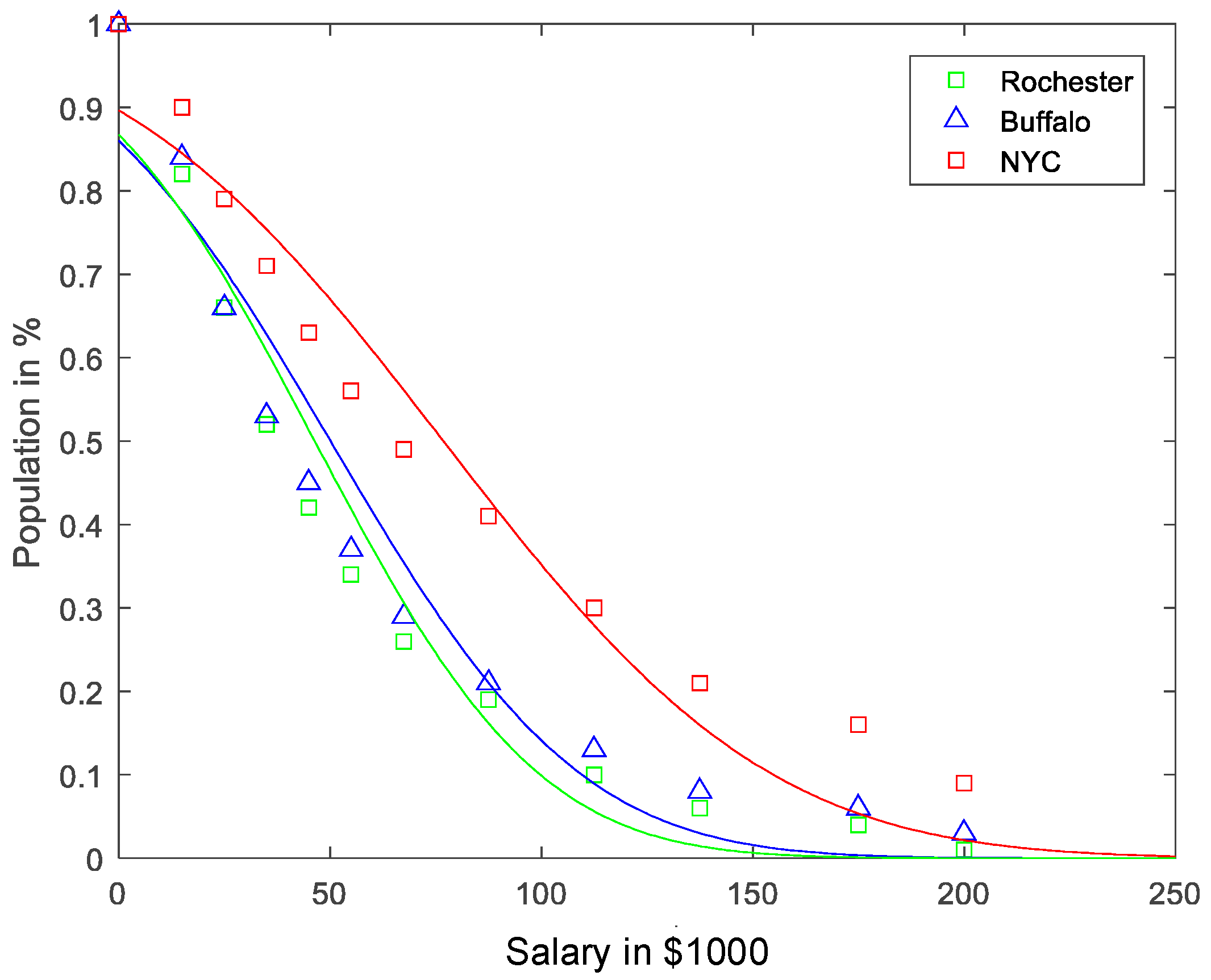
Figure 2.
Willingness-to-pay curves based on salary distribution at Buffalo, Rochester, and New York City when the load forecasts are all 80 MW.
Figure 2.
Willingness-to-pay curves based on salary distribution at Buffalo, Rochester, and New York City when the load forecasts are all 80 MW.

Figure 3.
Zonal prices of three areas during the last week of July 2018 in New York State; Buffalo, Rochester, NYC are included in West, Central, and NYC, respectively [11].
Figure 3.
Zonal prices of three areas during the last week of July 2018 in New York State; Buffalo, Rochester, NYC are included in West, Central, and NYC, respectively [11].

Figure 4.
One-line diagram of IEEE 3-Bus.
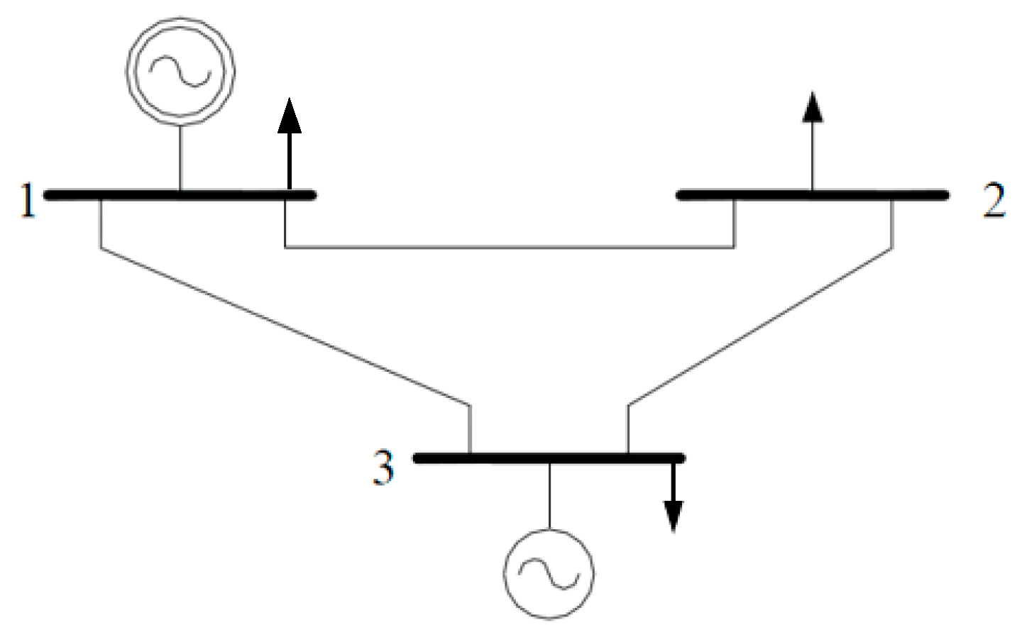
Figure 5.
Production costs of the generators located at Bus 1 and Bus 3, .

Figure 6.
State space diagrams shown at different angles for IEEE 3-Bus case where the x-mark stands for the current dispatch.
Figure 6.
State space diagrams shown at different angles for IEEE 3-Bus case where the x-mark stands for the current dispatch.

Figure 7.
One-line diagram of the reduced IEEE 30-bus system.

Figure 8.
Equi-cost contour plots as a function of two variable loads in the IEEE 30-bus system; Bus 1 and 4.
Figure 8.
Equi-cost contour plots as a function of two variable loads in the IEEE 30-bus system; Bus 1 and 4.
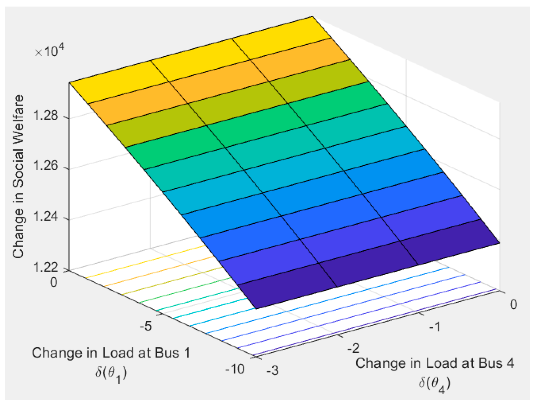
Figure 9.
Equi-cost contour of social welfare as a function of two variable loads in the IEEE 3-bus system.
Figure 9.
Equi-cost contour of social welfare as a function of two variable loads in the IEEE 3-bus system.


Table 1.
Salary and demographic information of Rochester, Buffalo, and NYC.
| Population [9] | Area in Mile 2 | Average Salary, μ | Standard Deviation, σ | |
|---|---|---|---|---|
| Rochester | 208,880 | 37.1 | $46,410 | $41,630 |
| New York City | 8,175,133 | 468.4 | $76,820 | $60,900 |
| Buffalo | 256,902 | 52.5 | $50,120 | $46,420 |
© 2018 by the author. Licensee MDPI, Basel, Switzerland. This article is an open access article distributed under the terms and conditions of the Creative Commons Attribution (CC BY) license (http://creativecommons.org/licenses/by/4.0/).
Share and Cite
MDPI and ACS Style
Oh, H. Demand-Side Management with a State Space Consideration. Energies 2018, 11, 2444. https://doi.org/10.3390/en11092444
AMA Style
Oh H. Demand-Side Management with a State Space Consideration. Energies. 2018; 11(9):2444. https://doi.org/10.3390/en11092444
Chicago/Turabian StyleOh, HyungSeon. 2018. "Demand-Side Management with a State Space Consideration" Energies 11, no. 9: 2444. https://doi.org/10.3390/en11092444
Note that from the first issue of 2016, this journal uses article numbers instead of page numbers. See further details here.