A Statistical Modeling Methodology for Long-Term Wind Generation and Power Ramp Simulations in New Generation Locations

Abstract

In future power systems, a large share of the energy will be generated with wind power plants (WPPs) and other renewable energy sources. With the increasing wind power penetration, the variability of the net generation in the system increases. Consequently, it is imperative to be able to assess and model the behavior of the WPP generation in detail. This paper presents an improved methodology for the detailed statistical modeling of wind power generation from multiple new WPPs without measurement data. A vector autoregressive based methodology, which can be applied to long-term Monte Carlo simulations of existing and new WPPs, is proposed. The proposed model improves the performance of the existing methodology and can more accurately analyze the temporal correlation structure of aggregated wind generation at the system level. This enables the model to assess the impact of new WPPs on the wind power ramp rates in a power system. To evaluate the performance of the proposed methodology, it is verified against hourly wind speed measurements from six locations in Finland and the aggregated wind power generation from Finland in 2015. Furthermore, a case study analyzing the impact of the geographical distribution of WPPs on wind power ramps is included.

1. Introduction

Wind power generation modeling has been a popular research topic in recent years since the installed wind generation capacities have been increasing rapidly in numerous countries. In the future, if CO₂ emissions are to be reduced globally, an even larger share of electricity will have to be generated from renewable sources including wind power. However, the increasing penetration of wind power in the power systems gives rise to increasing variation and power ramps in the net power generation. Methods for analyzing the effects of a large number of WPPs on the power ramps in future power systems are, thus, becoming increasingly important.

Long-term stochastic simulation of wind power to analyze WPPs and their variability has been a popular approach [1,2,3]. A frequently applied method in such modeling is to utilize Monte Carlo simulations for scenario analysis [2,3,4]. It has been common to utilize copulas in the stochastic modeling of wind generation in multiple WPPs. This allows the separation of modeling from the dependency structures of the WPPs, i.e., the temporal and spatial correlations from the modeling of the marginal probability distributions, i.e., margins of the individual WPPs [2,3,4,5]. A similar modeling approach is also used in this paper.

It is relatively straightforward to fit a time series model, e.g., an autoregressive model, or an artificial neural network (ANN) to a dataset covering existing locations [6,7,8,9,10], whereby the parameters of the time series model are estimated so that the important spatial and temporal characteristics of the data are modeled with some level of accuracy. However, as was shown in Reference [11], it is not straightforward to estimate the coefficients of a vector autoregressive (VAR) model when modeling new locations without measurement data (i.e., non-measured locations). This is because, in a full VAR model (i.e., a VAR model where no coefficients are assumed to be zero), the individual coefficients of the model cannot be said to contribute either to only spatial correlations or to only temporal correlations [8].

To overcome this challenge, one approach is to specify a simpler time series model where the coefficients of the model specify either temporal or spatial characteristics [11,12,13]. For example, in References [14,15], the VAR model was simplified so that the non-diagonal components of the VAR coefficient matrices were assumed to be zero (i.e., the simplified VAR model). This allows for a straightforward estimation of the model for new locations. This paper will show, however, that such a simplification may result in significant errors in simulated ramp rates. To tackle this problem, the use of the full VAR model is proposed along with a new estimation method that is suitable for modeling new locations.

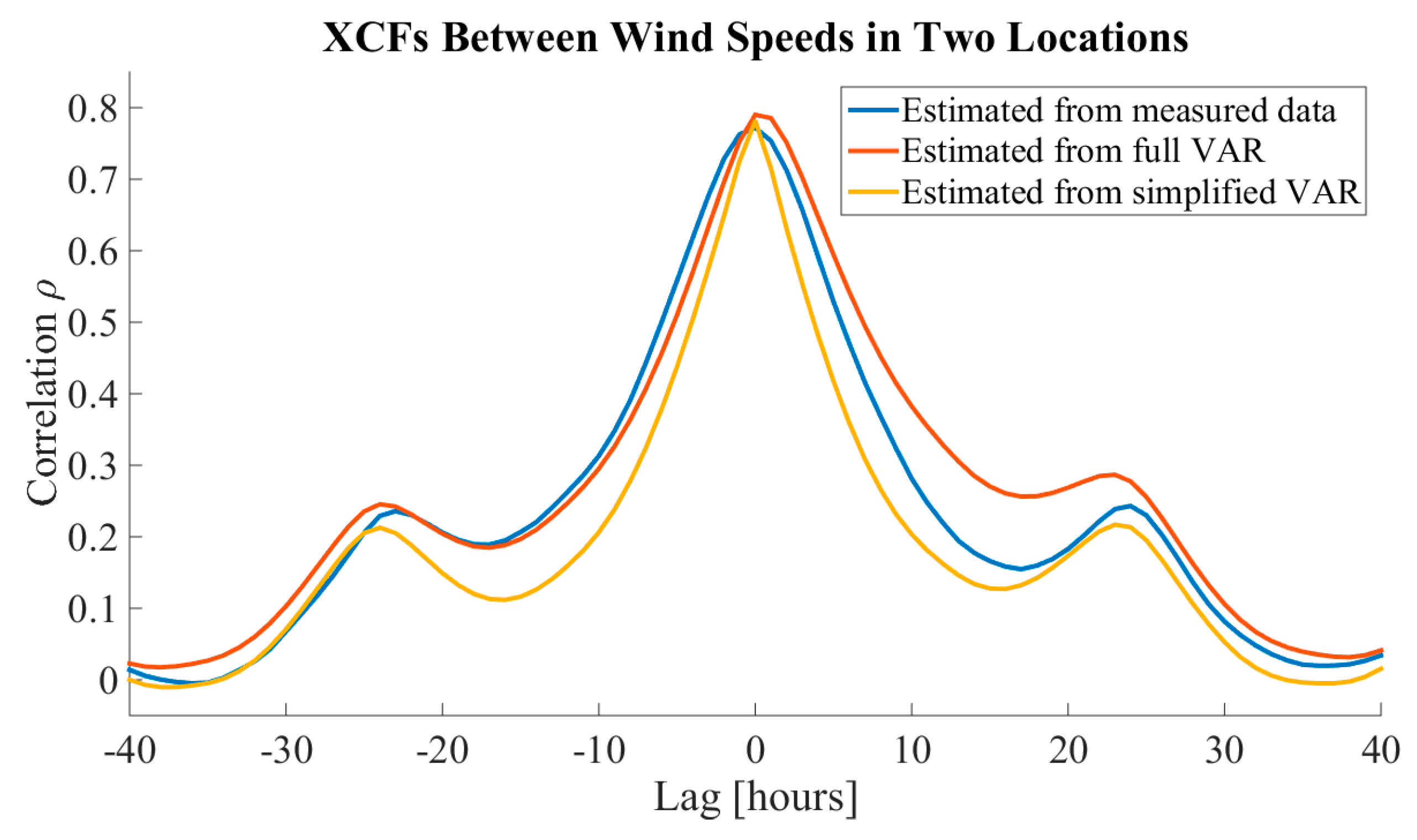
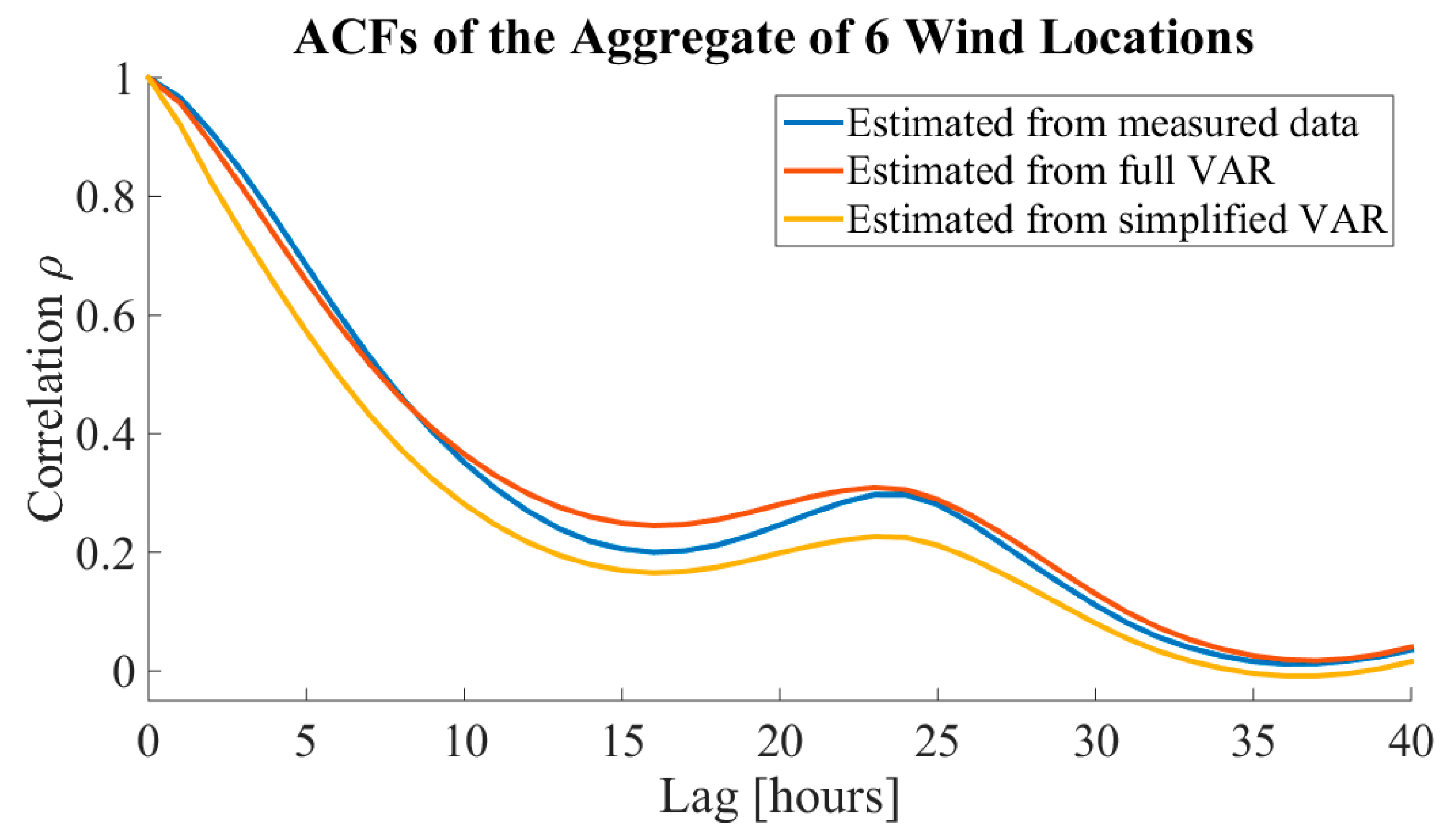
In previous research, a simplified VAR model has been unable to model the shape of the cross-correlation function (XCF) between two WPP locations [11,12]. Failure to model the XCFs between individual WPPs correctly, especially near lag 0, affects the modeling of the autocorrelation function (ACF) of the aggregated wind power generation, which will be shown in this paper. However, the proposed full VAR model can capture the correct shape of the spatial correlation structure between two locations with greater accuracy, which is important for the assessment of the aggregated power generation of multiple WPPs. In addition, the proposed VAR model can be estimated using only wind speed measurement data, which is not the case with many previously published approaches, such as in References [12,16].

The simplified VAR model is also used in wind and solar forecast simulations [17,18,19]. While this paper focuses on the simulation of wind generation, the presented full VAR model can also be considered for forecast simulations, where the use of a simplified time series model can have similar drawbacks, to those demonstrated in this paper for wind generation.

Furthermore, for the wind power generation model used to transform the simulated wind speeds to wind power instead of a commonly used third degree power curve [20], a state-of-the-art approach based on logistic functions [21,22] was used. The utilized approach allows for a deterministic estimation of detailed turbine specific power curves from the turbine data sheet parameters, which is essential when modeling non-measured WPPs.

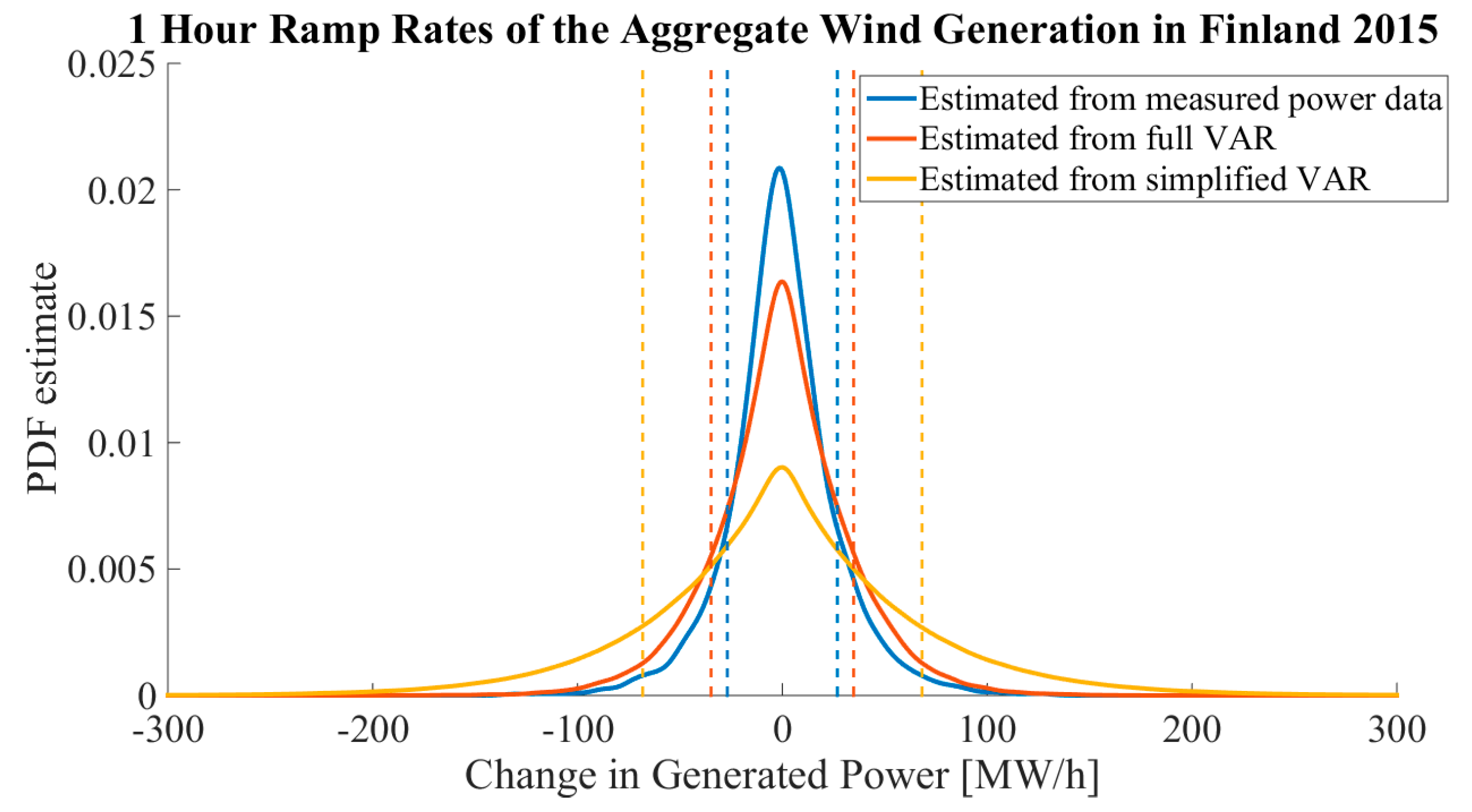
To summarize the contribution to the literature, the proposed VAR model enables a more accurate modeling of both the temporal correlations in individual WPPs and the spatial correlations between the WPPs in new locations. It is demonstrated that the autocorrelations of the aggregated power generation depend on the spatial correlations between the individual WPP locations, which can be modeled accurately with the full VAR model. Consequently, the proposed model can be utilized in the analysis of aggregated generation in future energy systems, including the detailed analysis of wind power ramp rates. It is shown that, with the new methodology, the estimation of the ACF of the aggregated generation and ramp rate probability distribution are much more accurate than with the previous approaches [12,15] that utilized the simplified VAR model.

This paper is organized as follows. Section 2 demonstrates the relation between the autocorrelations of an aggregated time series and the cross-correlations of the individual time series. Section 3 presents the proposed full VAR model and the specification of the model parameters for the analysis of temporal and spatial dependency structures. Section 4 describes the estimation data and the estimation of the simulation parameters and illustrates the overall structure of the methodology to model non-measured WPP locations. Section 5 presents the simulation results for six out-of-sample wind speed locations. Section 6 describes the power generation model used in the power simulations. Section 7 introduces the simulation results for out-of-sample modeling of the aggregated wind power generation in Finland in 2015. Section 8 presents the results for a case study assessing the impact of the geographical distribution of the WPP locations on the wind power ramp rates and Section 9 concludes the paper.

2. The Impact of the Cross-Correlations of Individual Time Series on the Autocorrelations of Their Sum

This section shows that the autocorrelation of a sum of multiple time series depends on the cross-correlations between the individual time series. Consequently, it highlights the importance of using a full VAR model in the modeling of aggregated wind power generation, since it is able to model the shape of the XCF near lag 0, which is shown in Section 5.2.

Next, a simple example to demonstrate the dependency between the cross-correlations of two stationary time series $y_{1,t}$ and $y_{2,t}$ and the autocorrelation of their sum $y_t=y_{1,t}+y_{2,t}$ is presented for lag h = 1. The autocorrelation of the aggregated time series $y_t$ can be specified for lag h = 1 as shown in the equation below.

$$cor\left(y_t,y_{t-1}\right)=\frac{cov\left(y_t,y_{t-1}\right)}{Var\left(y_t\right)}$$

(1)

On the other hand, according to the properties of covariance

$$cov\left(y_t,y_{t-1}\right)=cov\left(y_{1,t},y_{1,t-1}\right)+cov\left(y_{1,t},y_{2,t-1}\right)+cov\left(y_{2,t},y_{1,t-1}\right)+cov\left(y_{2,t},y_{2,t-1}\right)$$

(2)

and the variance of a sum of two random variables is given by

$$Var\left(y_t\right)=Var\left(y_{1,t}\right)+Var\left(y_{2,t}\right)+2cov\left(y_{1,t},y_{2,t}\right)$$

(3)

Using Equations (2) and (3) and the relation between covariance and correlation $cov\left(y_{1,t},y_{2,t}\right)=cor\left(y_{1,t},y_{2,t}\right){\sigma }_{y1}{\sigma }_{y2}$, Equation (1) can be expressed with the correlations between $y_{1,t}$ and $y_{2,t}$ as shown below.

$$cor\left(y_t,y_{t-1}\right)=\frac{cor\left(y_{1,t},y_{1,t-1}\right){\sigma }_{y1}^2+{\sigma }_{y1}{\sigma }_{y2}\left[cor\left(y_{1,t},y_{2,t-1}\right)+cor\left(y_{2,t},y_{1,t-1}\right)\right]+cor\left(y_{2,t},y_{2,t-1}\right){\sigma }_{y2}^2}{{\sigma }_{y1}^2+{\sigma }_{y2}^2+2cor\left(y_{1,t},y_{2,t}\right){\sigma }_{y1}{\sigma }_{y2}}$$

(4)

where $\sigma$ is the standard deviation (STD) of the corresponding time series. As shown in Equation (4), the cross-correlations between time series $y_{1,t}$ and $y_{2,t}$ with lags −1 and 1 (as XCF is asymmetric with respect to 0) affect the autocorrelation of the aggregated time series $y_t$ at lag 1.

Consequently, a similar dependency between the cross-correlations of individual time series and the autocorrelations of their aggregate occurs with multiple time series and for all lags. Hence, it is crucial to be able to model the cross-correlations between individual non-measured WPP locations as accurately as possible in order to capture the correct behavior of the ACF of the aggregated time series for the WPP locations.

3. The Modeling of the Temporal and Spatial Dependency Structures

This section presents the full VAR model and the specification of the model parameters.

3.1. The Vector Autoregressive Model

A k-dimensional VAR model with order p, i.e., a VAR_k(p) model for a process $z_t={\left[z_{1,t},z_{2,t},\dots ,z_{k,t}\right]}^{\prime }$ is specified by the equation below.

$$z_t=c+{{\displaystyle \sum }}_{h=1}^p{A}_h{z}_{t-h}+u_t,$$

(5)

where c is a $k\times 1$-dimensional vector of intercept terms, $A_1,..,A_p$ are $k\times k$-dimensional VAR coefficient matrices and $u_t={\left[u_{1,t},u_{2,t},\dots ,u_{k,t}\right]}^{\prime }$ is the error term of the VAR model [23]. The error term $u_t$ is a white noise process, i.e., it has zero mean and no correlation between the components when lag h ≠ 0.

In the VAR model presented in this paper, the margins of the error terms $u_t$ are assumed to follow Student’s t-distribution and the correlations between the components of $u_t$ are modeled with a Gaussian copula. The use of t-distributions for the error term margins is justified in References [12,15,16]. In addition, the intercept terms are assumed to be zero (c = 0). In the proposed model, the VAR coefficient matrices $A_1,..,A_p$ are fully specified without any components assigned to zero, which is shown below.

$$A_h=\left[\begin{array}{cc}\begin{array}{cc}{a}_{h;1,1}& a_{h;1,2}\\ a_{h;2,1}& a_{h;2,2}\end{array}& \begin{array}{cc}\cdots & a_{h;1,k}\\ \cdots & a_{h;2,k}\end{array}\\ \begin{array}{cc}⋮& ⋮\\ a_{h;k,1}& a_{h;k,2}\end{array}& \begin{array}{cc}\ddots & ⋮\\ \cdots & a_{h;k,k}\end{array}\end{array}\right],$$

(6)

where, e.g., $a_{h;1,k}$, is the coefficient between $z_{1,t}$ and $z_{k,t}$ at lag h.

3.2. The Specification of the VAR Model Parameters

In this section, the method to specify the required VAR model parameters, i.e., the VAR coefficient matrices and the covariance matrix of the error terms ${\sum }_u$, is described in detail. The process to specify the model parameters starts with the estimation of autocorrelation matrices $R_z\left(h\right)$ for the process $z_t$, which is described in detail in Section 4.2. After the autocorrelation matrices $R_z\left(h\right)$ are estimated, they can be transformed to autocovariance matrices ${\Gamma }_z\left(h\right)$ using the equation below.

$${\Gamma }_z\left(h\right)=D{R}_z\left(h\right)D,$$

(7)

where D is a $k\times k$-dimensional diagonal matrix with the STDs of the components of $z_t$ on the diagonal.

Next, the VAR coefficient matrices are specified utilizing the obtained autocovariance matrices ${\Gamma }_z\left(h\right)$ and the Yule-Walker equations. The Yule-Walker equations, for lags h > 0, can be formulated as shown below.

$${\Gamma }_z\left(h\right)=A_1{\Gamma }_z\left(h-1\right)+\dots +A_p{\Gamma }_z\left(h-p\right),$$

(8)

where $A_1,\dots ,A_p$ are the VAR coefficient matrices and p is the order of the VAR model [23]. Equation (8), describing the relation between VAR parameters and autocovariance matrices as a function of lag h, can be written in the following form using basic matrix multiplication.

$${\Gamma }_z\left(h\right)=\left[A_1,\dots ,A_p\right]\left[\begin{array}{c}{\Gamma }_z\left(h-1\right)\\ ⋮\\ {\Gamma }_z\left(h-p\right)\end{array}\right].$$

(9)

According to [23], Equation (9) can be further formulated by the equation below.

$$\left[{\Gamma }_z\left(1\right),\dots ,{\Gamma }_z\left(p\right)\right]=\left[A_1,\dots ,A_p\right]\left[\begin{array}{ccc}{\Gamma }_z\left(0\right)& \dots & {\Gamma }_z\left(p-1\right)\\ ⋮& \ddots & ⋮\\ {\Gamma }_z\left(-p+1\right)& \dots & {\Gamma }_z\left(0\right)\end{array}\right],$$

(10)

which, on the other hand, is equivalent to the formula below.

$$\left[{\Gamma }_z\left(1\right),\dots ,{\Gamma }_z\left(p\right)\right]=A{\Gamma }_Z\left(0\right),$$

(11)

where ${\Gamma }_Z\left(0\right)$ is the autocovariance matrix of the process $z_t$ at lag 0 and A is the $kp\times kp$-dimensional VAR coefficient matrix of $z_t$ both in the ${\mathrm{VAR}}_{kp}\left(1\right)$ form, i.e., in the state-space representation. The state-space representation allows any VAR_k(p) process to be written in a $kp$-dimensional ${\mathrm{VAR}}_{kp}\left(1\right)$ form [22]. A is composed from the VAR coefficient matrices $A_1,\dots ,A_p$ as shown below.

$$A=\left[\begin{array}{ccc}{A}_1& A_3& \begin{array}{ccc}\dots & A_{p-1}& A_p\end{array}\\ I_k& 0& \begin{array}{ccc}\dots & 0& 0\end{array}\\ \begin{array}{c}0\\ ⋮\\ 0\end{array}& \begin{array}{c}{I}_k\\ ⋮\\ 0\end{array}& \begin{array}{ccc}\dots & 0& 0\\ \ddots & ⋮& ⋮\\ \dots & I_k& 0\end{array}\end{array}\right],$$

(12)

where $I_k$ is a $k\times k$-dimensional identity matrix. Since matrix A is needed to specify the VAR model for the simulations, it can be solved from Equation (11) with the following formulation.

$$A=\left[{\Gamma }_z\left(1\right),\dots ,{\Gamma }_z\left(p\right)\right]{\Gamma }_Z{\left(0\right)}^{-1},$$

(13)

where ${\Gamma }_Z\left(0\right)$ is a nonsingular matrix. Equation (13) defines the relation between the VAR coefficient matrix A and the autocovariance matrices of the process $z_t$ without any additional variables. Therefore, with Equation (13), the VAR coefficient matrices from 1 to p can be estimated using the estimated autocovariance matrices.

The only model parameter not yet specified is the covariance matrix of the error terms ${\sum }_u$, which can be determined from the Yule-Walker equations if the aforementioned VAR coefficient matrix A, which is specified in Equation (12), and the autocovariance matrices ${\Gamma }_z\left(h\right)$ are given. According to [23], the ${\mathrm{VAR}}_{kp}\left(1\right)$ form of the $kp\times kp$-dimensional covariance matrix of the error terms ${\sum }_U$ can be obtained by using the equation below.

$${\sum }_U={\Gamma }_Z\left(0\right)-A{\Gamma }_Z\left(0\right)A^{\prime }.$$

(14)

The $k\times k$-dimensional covariance matrix of the error terms ${\sum }_u$ can be obtained from the first k columns and k rows of ${\sum }_U$.

4. The Simulation of Non-Measured WPP Locations

This section presents the overall Monte Carlo (MC) simulation procedure for the modeling of non-measured WPP locations. First, the used data and the marginal distributions are described and, then, the estimation of the simulation parameters is presented. Lastly, the structure of the MC simulation procedure is presented step by step.

4.1. The Data and the Marginal Distributions

This paper utilizes the same wind speed datasets for the estimation of the VAR model as seen in References [12,15]. The datasets consist of hourly wind speed measurement time series from 12 high altitude locations (height from 74 to 150 m above the surrounding ground level) and 19 low altitude locations in Finland. The length of the measured time series varies from one to three years depending on location. It should be noted that the low altitude measurement data are used only in the estimation of the spatial and spatiotemporal correlations (as all 19 locations have the same measurement period of three years), which is explained in Section 4.2.

Empirical cumulative distribution functions (ECDFs) [3,16] are applied as margins for the wind speed measurement locations. The wind speed data from k measured locations denoted as $y_t={\left[y_{1,t},y_{2,t},\dots ,y_{k,t}\right]}^{\prime }$, are transformed to data with normally distributed margins $z_t^{wD}$ (where wD denotes with day structures, meaning that the monthly diurnal variations are still present in the data). The transformation to Gaussian data is performed by using the probability integral transformation.

$$z_{i,t}^{wD}=F_N^{-1}\left[{\widehat{F}}_i\left(y_{i,t}\right)\right],$$

(15)

where $F_N^{-1}$ is the inverse cumulative distribution function (CDF) of the standard normal distribution and ${\widehat{F}}_i$ is the estimated ECDF margin for location i.

Next, the monthly diurnal structures, i.e., the day structures, are estimated from $z_t^{wD}$ by calculating mean values for each hour of the day of each month. These means are subtracted from $z_t^{wD}$ and $z_t={\left[z_{1,t},z_{2,t},\dots ,z_{k,t}\right]}^{\prime }$ is obtained. The VAR model is then estimated from $z_t$. A similar approach has been used in Reference [15].

4.2. The Estimation of the VAR Model and Simulation Parameters for Non-Measured WPP Locations

The VAR model identification was achieved by assessing the ACFs and partial autocorrelation functions (PACFs) of $z_t$, which indicated that a suitable order for the VAR model was p = 4. The adequacy of the VAR_k(4) model, fitted for $z_t$, was verified by checking that the model residuals $u_t$ had no statistically significant ACF, PACF, or XCF values (except XCF with lag $h=0,$ which is acceptable). The margins of $u_t$ had too high kurtoses in all estimation locations to follow a normal distribution. Hence, t-distributions were fitted for the margins of the residuals.

When p = 4, the autocovariance matrices ${\Gamma }_z\left(h\right)$ are needed for lags $h=0,\dots ,4$ for the estimation of the VAR coefficient matrices, which is shown in Equation (13), and for the estimation of the covariance matrix of the error terms ${\sum }_u$, which is shown in Equation (14). The autocovariance matrices ${\Gamma }_z\left(h\right)$ are obtained from the autocorrelation matrices $R_z\left(h\right)$ with Equation (7). The STDs for the diagonal matrix D for new locations, which are used to convert $R_z\left(h\right)$ to ${\Gamma }_z\left(h\right)$ in (7), are averages of the STDs calculated from $z_t$ used in the estimation.

The autocorrelation matrices $R_z\left(h\right)$ specify both the temporal and spatial correlations of $z_t.$ For the non-measured WPP locations, the temporal correlations (the diagonal components) of $R_z\left(h\right)$ for the lags $h=0,\dots ,4$ are the average values of the ACFs calculated from the components of ${\mathit{z}}_t$ used in estimation.

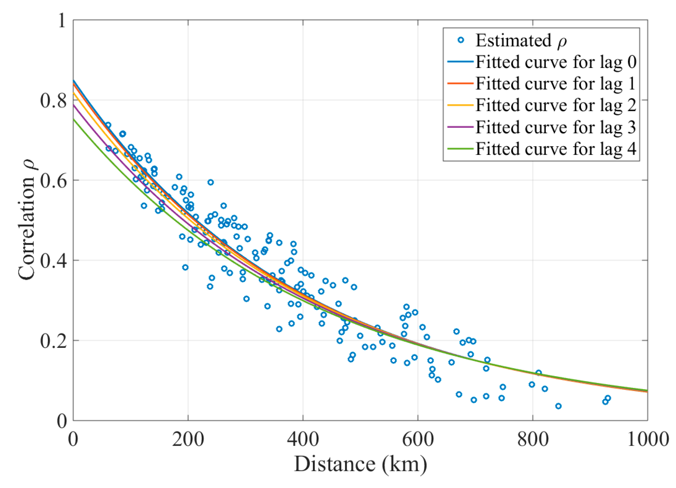
The spatial and spatiotemporal correlations (the off-diagonal components) of $R_z\left(h\right)$ are estimated by utilizing the distances between the non-measured WPP locations, which was done in [15]. Figure 1 illustrates the correlations (for h = 0) estimated from $z_t$ calculated for the 19 low altitude wind speed measurement locations against the distances between the measurement locations represented as blue circles. Figure 1 also shows the five curves fitted for these spatial and spatiotemporal correlations for lags $h=0,\dots ,4$. These five curves linking the distances between the locations to the corresponding spatial and spatiotemporal correlations are used to estimate the off-diagonal elements of $R_z\left(h\right)$ for lags $h=0,\dots ,4$ for the new locations.

The covariance matrix ${\sum }_u$, which is estimated and shown in Section 3.2., is modeled as a Gaussian copula. The mean value of the degrees of freedom from the fitted t-distributions (5.8068) is used to specify the margins of ${\sum }_u$ for the non-measured WPP locations.

The correlation matrix of the error terms $R_u$, which is derived from ${\sum }_u$, is used as the correlation matrix for the Gaussian copula, $R_{Gauss}$. This approximation showed very similar $R_{Gauss}$ and $R_u$ in the simulations and gave valid results in the applications, which are shown in Section 5 and Section 7.

The monthly diurnal variations, i.e., the day structures, are estimated from $z_t$ and used in the estimation, which is described in Section 4.1. The averages of the estimated day structures are used for the non-measured WPP locations. Weibull distributions commonly used to describe the wind speed conditions in a specific location [12] are applied as margins for the new WPP locations. The Weibull distribution parameters for each new location are obtained from the Wind Atlas database [24].

4.3. The Estimation of the VAR Model and Simulation Parameters for Non-Measured WPP Locations

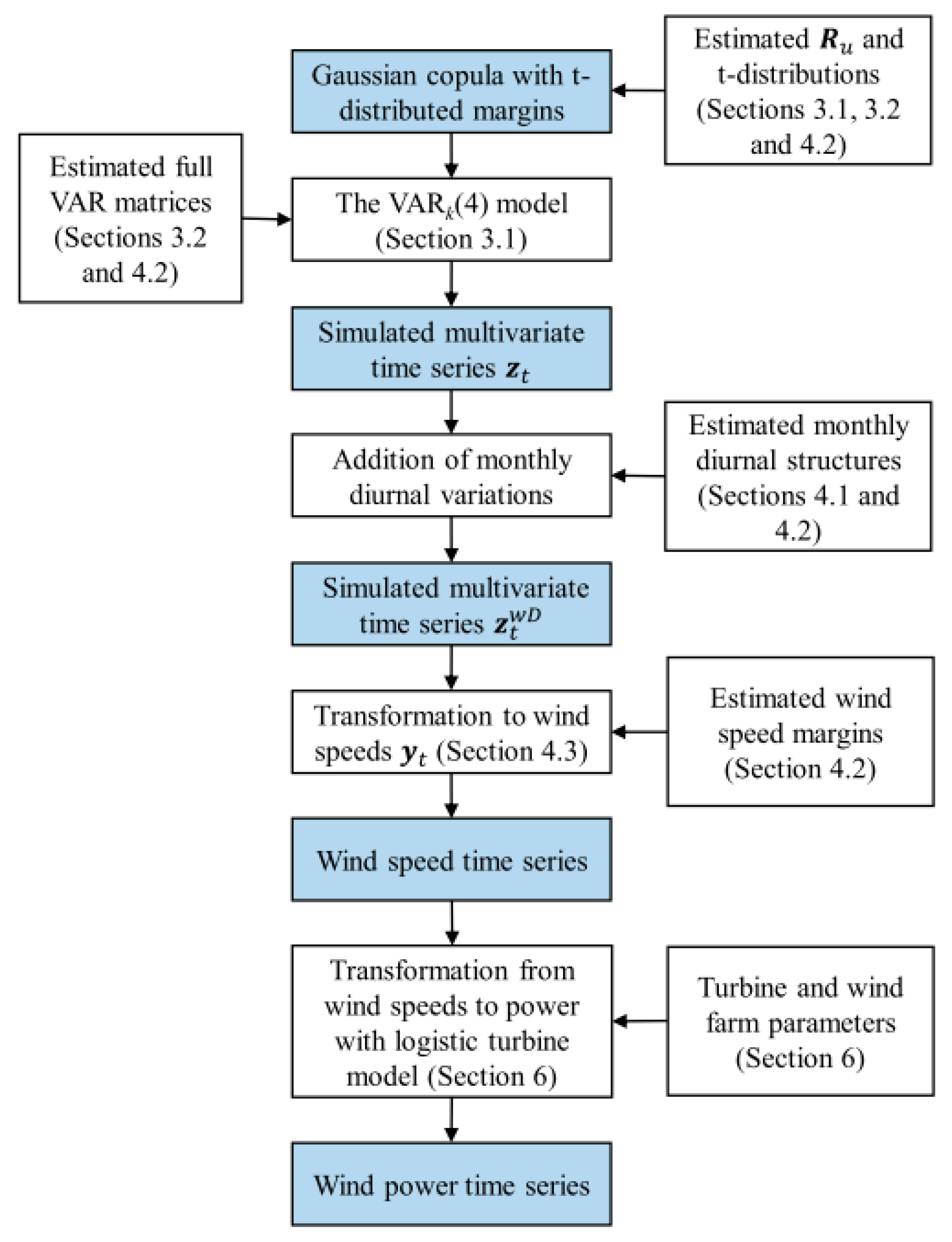
The simulation procedure is illustrated in Figure 2. The procedure begins with the drawing of a sample from the Gaussian copula for the k simulated WPP locations for the length of the simulation and transforming the margins to t-distributions.

Next, the correlated t-distributed random numbers are used as innovations for the VAR_k (4) model. The model produces a simulated multivariate time series $z_t$ with the appropriate spatial and temporal dependency structures. Then the estimated monthly diurnal structures are added to the simulated data, which yields $z_t^{wD}$. As Figure 2 shows, the simulated $z_t^{wD}$ is further transformed to wind speeds with the formula below.

$$y_{i,t}={\widehat{F}}_i^{-1}\left[F_N\left(z_{i,t}^{wD}\right)\right]$$

(16)

where $y_{i,t}$ is the resulting simulated wind speed in location i at time t, ${\widehat{F}}_i^{-1}$ is the estimated inverse CDF of the Weibull distributed wind speed margin for location i, and $F_N$ is the CDF of the standard normal distribution.

The last step in the procedure is to transform the multivariate wind speed time series $y_t$ to the power time series for each individual WPP using the wind power generation model presented in Section 6. The power time series for each WPP can be aggregated to a single time series depicting the aggregated wind power generation for the whole simulated system.

5. Monte Carlo Simulation Results for the Six Out-of-Sample Wind Speed Locations

This section introduces the MC simulation results for the long-term out-of-sample simulations for six high altitude wind speed locations in Finland. The proposed full VAR model is compared with the simplified VAR model, which is utilized with the same overall methodology.

5.1. The Simulation Setup for Out-of-Sample Wind Speed Simulations

The performance of the VAR model is compared with the simplified VAR model, which has been used previously in similar modeling. The simplified VAR model is a VAR model in which the off-diagonal components of the VAR-parameter matrices are assumed to be zeros [14,15].

The two models are estimated with the same data set of measured high altitude wind speed locations in Finland, which is presented in Section 4.1. The measured data from six simulated locations are left out of the estimation procedure, which provides the six out-of-sample locations used in the model validation.

Additionally, 100 MC simulation runs with a time resolution of one hour and a length of one year were performed. This yielded $8.76\times {10}^5$ samples for each of the six locations. The results presented in this section also consider the aggregated time series of these six locations to assess the models’ ability to simulate the properties of an aggregate of several locations. The reader should note that wind speed aggregation from several locations is carried out only for model evaluation purposes.

5.2. The Spatial Correlation Structures

Figure 3 illustrates the XCFs between two of the six test locations, which is estimated both from the measured data and from the simulated data from the two models. Both models can capture the peak of the XCFs at lag 0 relatively well. However, only the full VAR model can capture the round shape of the XCF estimated from the measured data. The XCF estimated from the simulation data of the simplified VAR model produces XCF values that are too low for most lags and a too peaked shape of the XCF around lag 0. This problem is the root cause for the poorer performance of the simplified VAR model. This is the next part presented in this section. The high XCF values for the full VAR model between lags 10 and 24 are caused by the average diurnal structures that are used for the out-of-sample test locations, as in one of the two considered locations the utilized average diurnal structure deviates from the actual diurnal structure.

5.3. The Temporal Correlation Structure of the Aggregate

The ACFs estimated from the aggregated measurement data and simulated data from the models are shown in Figure 4. It can be observed that the ACF estimated from the full VAR model has a very similar shape to the ACF estimated from the aggregated measurements and the most critical lags (the ones close to lag 0) are very close to each other. The simplified VAR model produces ACFs that are too low compared to the aggregated measurement data for all observed lags. This is caused by the relation between the ACF of the aggregated time series and the XCFs between the individual locations, which is discussed in Section 2.

5.4. The One Hour Ramp Rates of the Aggregate

The one-hour ramp rate PDFs and the STDs of the one-hour ramp rates estimated from the aggregated measurement data and simulated data from the two models are illustrated in Figure 5. The PDFs and STDs of the measurements and full VAR model simulations are very similar. The simplified VAR model is unable to capture the correct shape of the ramp rate PDF since the slope is too gentle and consequently the STD is also too large. This is due to the same reason as seen with the low ACF values compared with the measurement data in the previous subsection; namely, the simplified VAR model’s limited ability to model the XCFs between the individual locations, which results in ramp rate PDFs that have too gentle sloping.

6. The Wind Power Generation Model

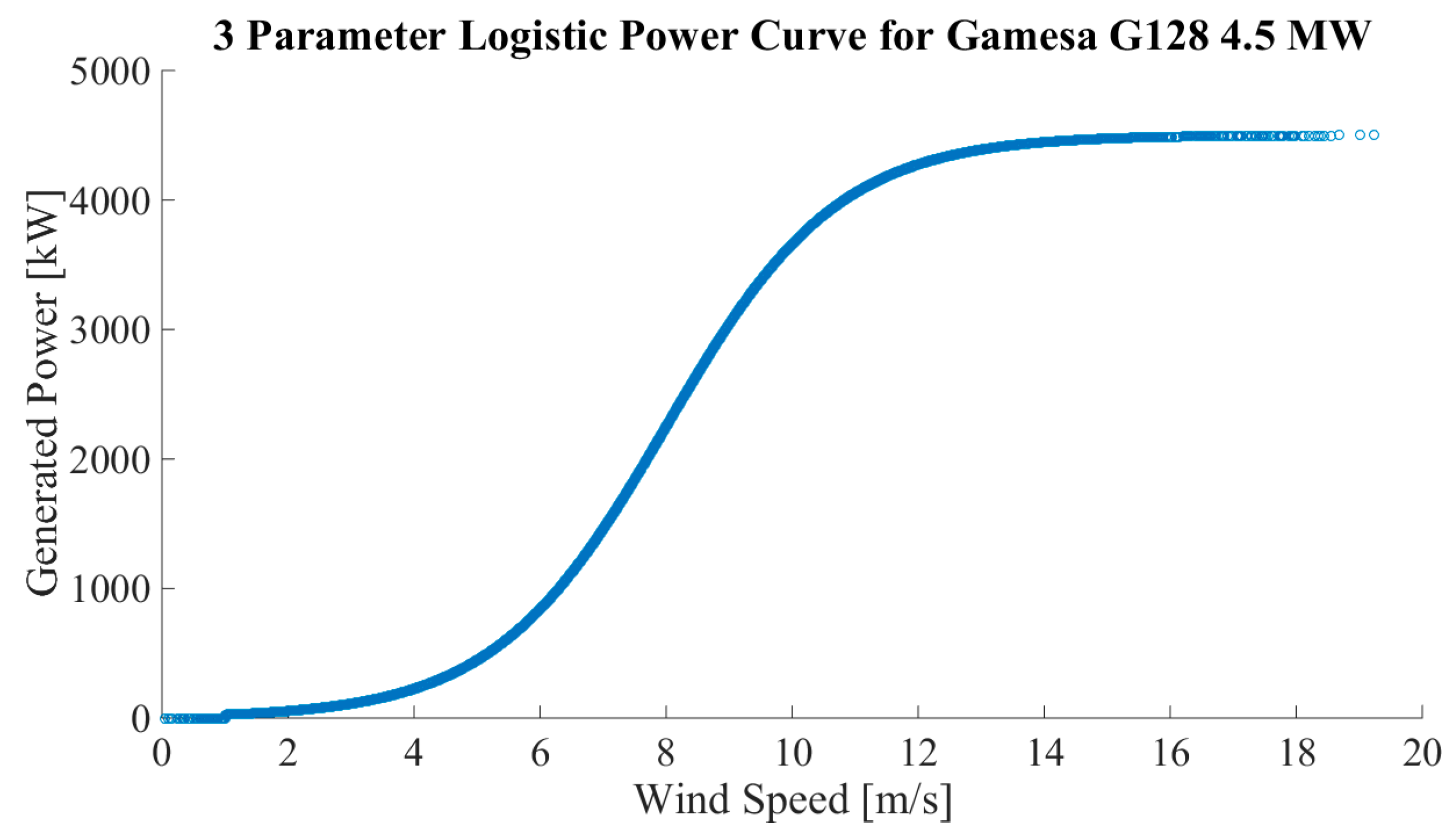
This section presents the power generation model to transform the simulated wind speeds to generated power. The paper utilizes an improved state-of-the-art power generation model based on a logistic function in the methodology [21]. For the wind turbine model, a three-parameter logistic power curve estimated using a deterministic process is utilized. This is proposed in Reference [22], where it is shown to perform better than other approaches. This particular approach was chosen as the parameters of the logistic function, which can be obtained using only information available from the wind turbine data sheets without any requirements for measured power generation data. The implemented logistic function to transform the wind speeds to generated power can be written using the formula below.

$$P\left(u\right)=\frac{P_r}{1+e^{4s\left(u_{ip}-u\right)/P_r}},$$

(17)

where $P_r$ is the rated power of the wind turbine, u is the wind speed, $u_{ip}$ is the wind speed in the inflection point, which is the point in the power curve where the gradient of the power is at its maximum, and s is the slope of the power curve in the inflection point, i.e., the value of the gradient. Equation (17) is applied between the specific cut-in and cut-out speeds specified for a turbine. An example of the shape of the power curve produced by the utilized turbine model is illustrated for the Gamesa G128 4.5 MW wind turbine [25] in Figure 6.

In addition, the wake effect, i.e., the slowed down and turbulent wind caused by turbines in the downwind direction inside a wind farm, is considered using a wake coefficient, which is presented in Reference [26], before aggregating the power generation of the individual turbines to give the power generation of the wind farm. The wake coefficient for a wind farm is determined based on the number of turbines in the farm and the distance between the turbines. When the farm topology is not known, e.g., with new wind farms, a regular array topology with the distance of nine times the rotor diameter between the turbines is assumed. A similar approach was used with new wind farms in Reference [12].

7. Monte Carlo Simulation Results for the Wind Power Generation Structure of Finland in 2015

This section introduces the MC simulation results for the long-term simulations for wind power generation in Finland during 2015. The performance of the full VAR model is compared with the simplified VAR model.

7.1. The Simulation Setup for Large Scale Wind Power Generation Simulations

Both the full VAR and simplified VAR models are estimated with the same data set of measured high altitude wind speeds from nine locations in Finland. The simulations are a complete out-of-sample test, i.e., no information from the generated power time series from 2015 is utilized in any way in the estimation of the models or in the simulations.

The simulations consider the changing installed capacity during 2015 from 622 MW to 1008 MW as well as the changing number of wind farms. At the end of 2015, there were 377 wind turbines in Finland, which are aggregated to 53 individual wind farms illustrated in Figure 7 for the simulations. All wind turbines are modeled individually according to their data sheet parameters, which is discussed in Section 6. A total of 100 MC simulation runs with a time resolution of one hour and length of one year were performed, yielding $8.76\times {10}^5$ samples for each of the 53 wind farms in Finland. The computational times for 100 MC simulation runs with this simulation setup were roughly 10 minutes for both the full and simplified VAR models.

All of the presented results in this section consider the aggregate generation of these 53 wind farms, which is compared with the measured aggregated wind power generation in Finland in 2015 obtained from the Finnish Energy Industries. The entire simulated wind power generation in Finland is aggregated to a single time series for each run after wind speeds are simulated for each wind farm and then transformed to the generated power for each turbine.

7.2. The Probability Density Functions

The PDFs estimated from the measured power generation data and from the data simulated with the models are presented in Figure 8. According to the figure, both of the simulation models manage to produce similar PDFs to the one estimated from the measured data. The only difference is that the models yield PDFs that deviate slightly from the data when the aggregated generation is very low. The mean values for the generation, depicted as dashed lines in Figure 8, are almost identical with the data for both models.

7.3. The Temporal Correlation Structures

The ACFs estimated from the measured power generation data and simulated data from the full VAR and simplified VAR models are illustrated in Figure 9. It can be seen from the figure that the ACFs estimated from the measurements and from the full VAR model simulations have a very similar shape. The ACF produced by the simplified VAR model is notably lower for all lags compared to the ACF of the measurements.

7.4. The One Hour Ramp Rates

Figure 10 illustrates the one-hour ramp rate PDFs and the STDs of the ramp rates estimated from the measured power generation data and aggregated data simulated with the two models. The PDFs and the STDs estimated from the measurements and from the full VAR model simulations are close to each other, even though the full VAR model estimate of the PDF is slightly more spread, which can be seen from both the PDF and the STD. However, the simulation results are still close to the measured data, especially considering that this is a complete out-of-sample simulation test. Similarly, as with the wind speeds in Section 5, the simplified VAR model is unable to capture the correct peaked shape of the one-hour ramp rate PDF since the slope of the PDF is significantly too gentle and, consequently, the STD is too large.

7.5. The Numerical Comparison

The most relevant numerical statistics are presented in

Table 1. The numerical statistics estimated from the measured aggregated wind power generation in Finland in 2015 and from the aggregated simulated data from the two models. σ stands for standard deviation and the capacity factor is the ratio between installed capacity (calculated with the maximum installed capacity at the end of 2015) and the actual output. The <20% and >80% rows show the percentage of hours in a simulation run when the aggregated generation is within the limits. The presented statistics estimated from the simulation results are averages of the 100 MC runs.

Statistic	Data	Full VAR	Simplified VAR
Yearly Energy (TWh)	2.33	2.33	2.33
Maximum Generation (MWh/h)	868.35	863.97	869.03
Capacity Factor (%)	0.26	0.26	0.26
Hourly σ (MWh/h)	185.59	182.15	180.08
<20% of installed capacity (%)	44.01	43.96	43.81
>80% of installed capacity (%)	0.39	0.26	0.22
ACF of the aggregate at lag 1	0.99	0.98	0.93
σ of the 1 h ramp rate (MWh/h)	26.84	34.83	68.21

. The statistics are estimated from the measured aggregated power generation and from the aggregated data simulated with the two simulation models. According to Table 1, both models perform well in most aspects of the modeling. There are, however, major differences in the modeling of the ACF and the STD of the ramp rates. The full VAR model also performs well in the modeling of the ACF at lag 1 (and also with other lags, as shown in Figure 9) and the STD of the one-hour ramp rate.

To summarize the results for the wind power generation in Finland in 2015, the full VAR model performs well in all studied measures and surpasses the simplified VAR model in the modeling of aggregate power generation of a large system. Most notably, the temporal dependency structures and ramp rates of the aggregate generation are modeled correctly, which is not the case with the simplified VAR. Therefore, the full VAR model can be considered as the superior choice for the modeling of wind power generation in multiple non-measured WPP locations.

8. The Comparison of the Ramp Rates of the Wind Generation with Different Geographical Distributions

In this section, two wind power generation scenarios are studied to analyze the effect of geographical distribution of the WPP locations on the aggregated wind power ramps. Two distinct geographical distributions of the WPPs are considered; dispersed and concentrated.

8.1. The Simulation Setup for the Scenarios

The two wind power generation scenarios consist of 12 WPPs with 20 Gamesa G128-4.5 turbines with 4.5 MW nominal power [25] in each, which results in 90 MW of total installed capacity per WPP. Hence, the aggregated installed capacity in both scenarios is 1080 MW. The hub height of the wind turbines is considered to be 140 m for all turbines.

In the first of the two scenarios, the locations of the WPPs are geographically dispersed and, in the second scenario, the locations are geographically concentrated. In the concentrated scenario, the average distance between the WPPs is 59.6 km and, in the dispersed scenario, the average distance is 285.6 km. In both scenarios, the WPPs are considered to be located in Southern and Central Finland.

To enable a more straightforward comparison of the scenarios in terms of the impact caused by the geographical distribution of the WPPs on the wind power ramps, the generation conditions are fixed in each WPP location. This means that the Weibull parameters describing the wind speed conditions are similar for each WPP in both scenarios. Consequently, the annual generated energy and the hourly mean generation are very similar for both scenarios. The utilized Weibull parameters (A = 8.5 and B = 2.3) are the averages of the parameters obtained for a height of 140 m from the Finnish Wind Atlas database [24] for the WPPs in Section 7.

8.2. The Simulation Results for the Scenarios

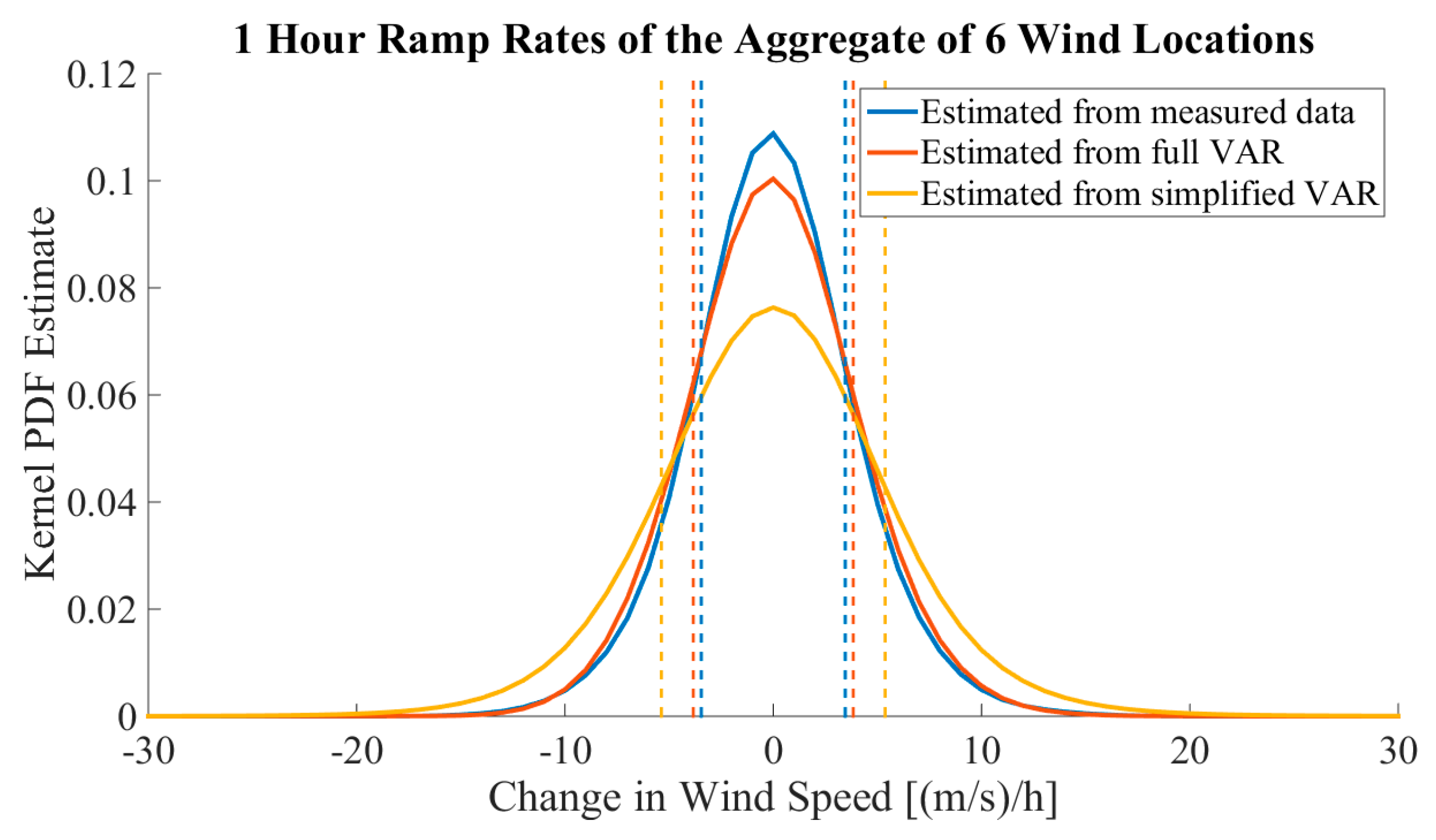
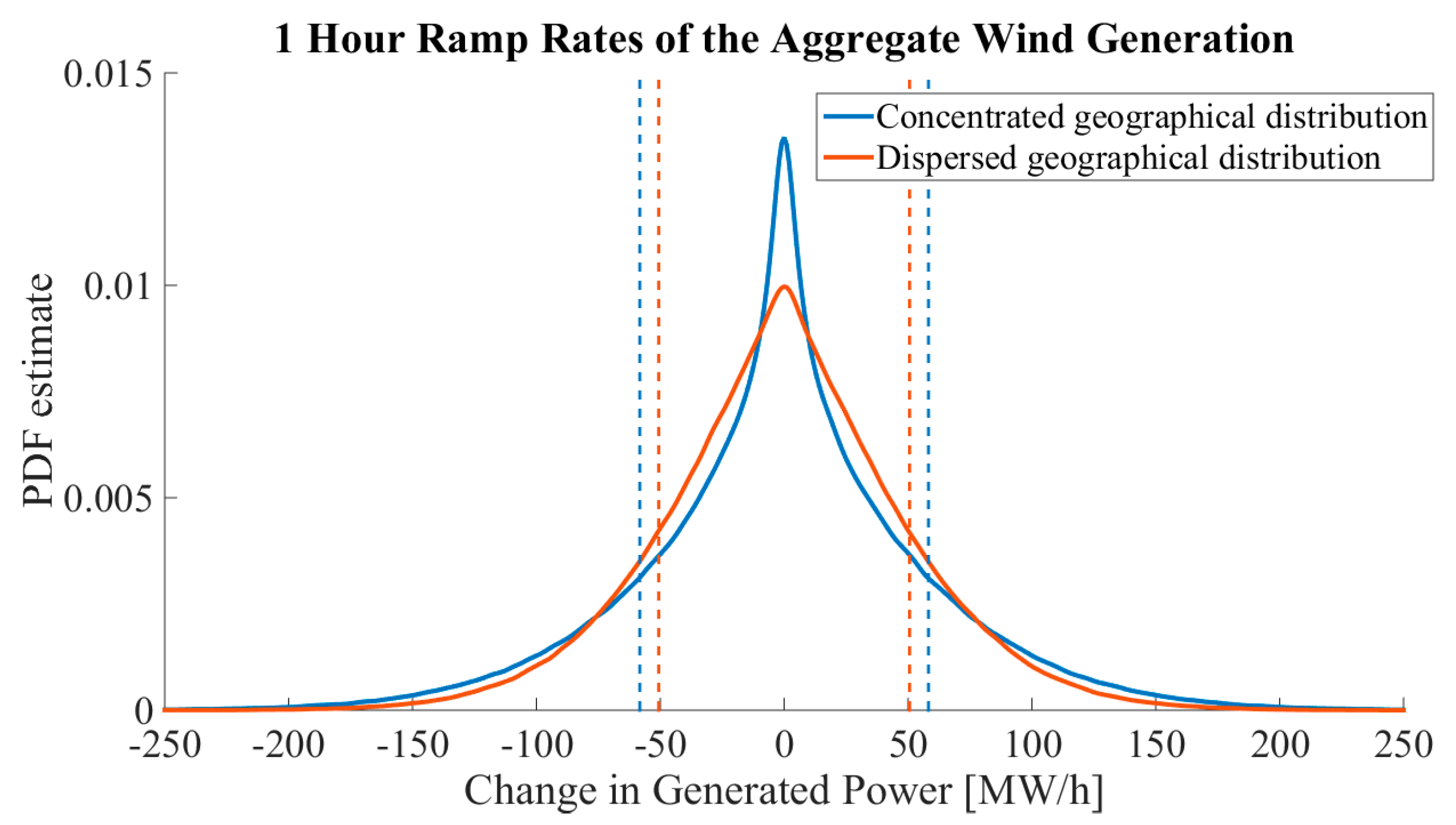
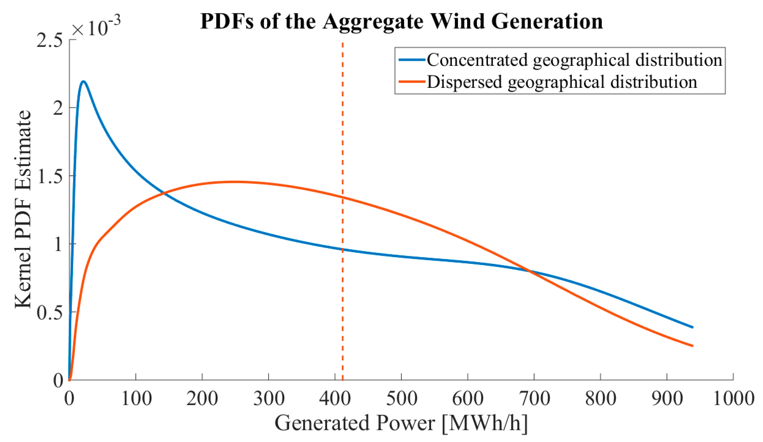
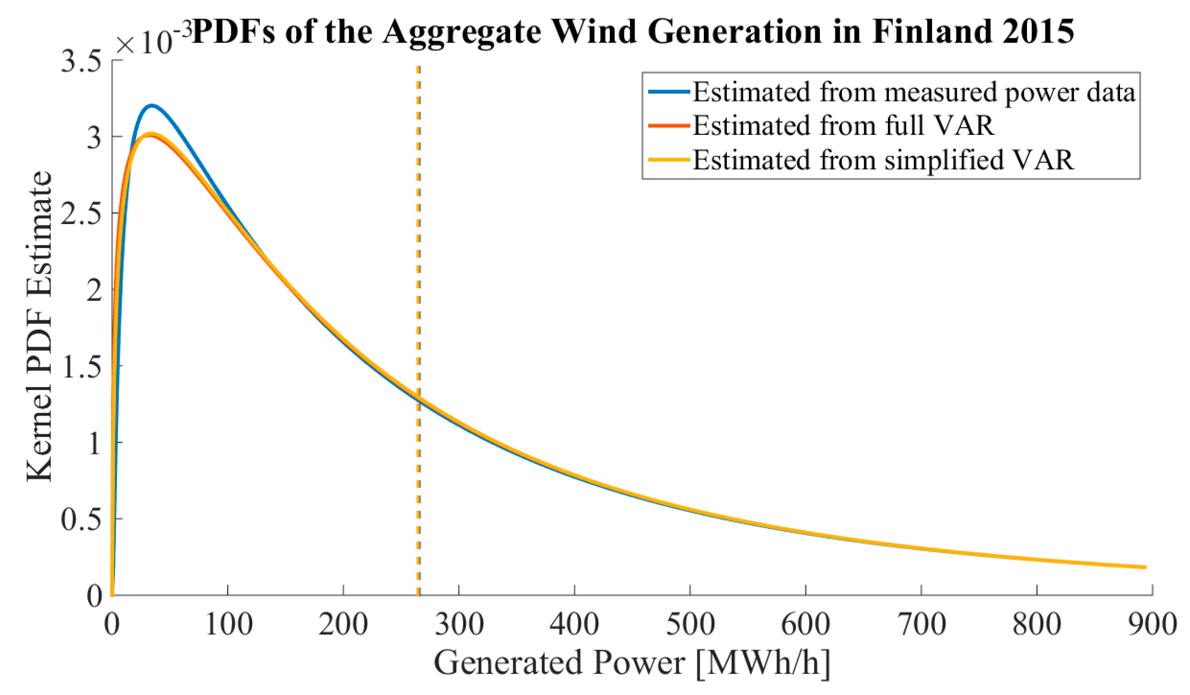
This section presents the aggregated MC simulation results for the two scenarios. A total of 100 MC simulation runs were performed with an hourly time resolution, resulting in $8.76\times {10}^5$ simulated samples for each WPP in both scenarios. The simulation results for the aggregated power generation are illustrated for one-hour ramp rate PDFs in Figure 11 and for power generation PDFs in Figure 12.

Table 2. The numerical statistics estimated from the aggregated wind power generation with dispersed and concentrated geographical distribution. The <10%, <20%, and >80% rows show the percentage of hours in a simulation run when the aggregated generation or the one-hour ramp rates are within the respective limits. The presented statistics estimated from the simulation results are averages of the 100 MC runs.

Statistic	Dispersed Geographical Distribution	Concentrated Geographical Distribution
Yearly Energy (TWh)	3.61	3.61
Hourly Mean (MWh/h)	411.67	411.56
Generation <20% of installed capacity (%)	24.73	32.89
Generation >80% of installed capacity (%)	2.33	7.28
Hourly σ (MWh/h)	233.18	283.24
1 h up or down ramp <10% of installed capacity (%)	4.16	7.69
1 h up or down ramp <20% of installed capacity (%)	0.03	0.22

presents the numerical results obtained for the scenarios.

As Figure 11 shows, the geographical distribution does have a significant impact on the shape of the one-hour ramp rate PDFs. It is clear that the dispersed scenario yields smaller hourly volatility for the one-hour ramp rates compared to the concentrated scenario. The power generation PDFs in Figure 12 show that, in the geographically dispersed scenario, the hourly generation has smaller volatility and fewer hours with a very large or small aggregated generation, which is in line with previous research, as shown in References [11,12,14,16].

In addition, according to Table 2, the yearly energy and hourly mean generation are similar in both scenarios, which is expected. In the geographically concentrated scenario, extreme generation events, with aggregated generation less than 20% or more than 80% of the installed generation capacity, are more likely (also visible in Figure 12). In addition, the STD of the aggregated generation is notably smaller in the geographically dispersed scenario. The probabilities for ramp rates being more than 10% or 20% of the installed capacity are larger with the concentrated distribution, which is also visible from Figure 11. In addition,

Table 3. The standard deviations (σ) of the ramp rates for different ramp lengths with dispersed and concentrated geographical distribution. The results are averages of the 100 MC runs.

Statistic	Dispersed Geographical Distribution	Concentrated Geographical Distribution
σ of the 1 h ramp rate (MW/h)	50.63	58.25
σ of the 2 h ramp rate (MW/h)	70.84	88.34
σ of the 3 h ramp rate (MW/h)	88.40	113.31
σ of the 4 h ramp rate (MW/h)	101.28	133.53
σ of the 5 h ramp rate (MW/h)	112.53	150.21
σ of the 10 h ramp rate (MW/h)	146.55	200.27

presents the STDs of the ramp rates for different ramp lengths from 1 hour to 10 hours. The ramp rates of the dispersed generation are notably lower, regardless of the length of the ramp rate. The differences between the two scenarios increase when looking at longer ramp lengths.

To summarize, the STDs of the ramp rates and the probabilities for very large up or down power ramps are notably smaller with the geographically dispersed scenario. Hence, the dispersed placement of WPPs results in smaller ramp rates and, thus, easier manageability of the power ramps from the perspective of the power system operator.

9. Conclusions

This paper has presented an improved VAR model based methodology to model wind power generation in multiple new WPP locations. It was shown that the detailed modeling of temporal correlations in individual WPP locations and the spatial correlations between the WPPs are essential in order to properly model the dependency structures of the aggregated power generation. It was demonstrated that the proposed model is able to model the correlational structures with required accuracy for the analysis of aggregated wind power generation and power ramps. Furthermore, an estimation method suitable for the modeling of new WPP locations was presented for the proposed full VAR model.

The ability of the proposed methodology to model the aggregated generation of non-measured WPP locations was verified both in wind speed and wind power domains against measured data. An aggregate of six out-of-sample wind locations and the aggregated wind power generation in Finland in 2015 were modeled and the simulations compared well with the measured data. The model was able to simulate aggregated time series with similar statistical qualities and dependency structures to those present in the measured data in both studied cases and was found to be superior to the simplified VAR model.

The presented VAR model extends the applicability of the existing methodology to cover detailed long-term simulations and scenario analyses of the volatility of the future wind power generation including wind power ramp analysis. The detailed analysis of power ramps and especially the assessment of the impact of new WPPs on the aggregated power ramps are crucial topics for both transmission system operators and power producers.

Lastly, a case study assessing the impact of the geographical distribution of the WPP locations on the aggregated ramp rates was presented. The paper quantifiably verified that the impact of the geographical distribution is significant on the aggregated ramp rates and that dispersed geographical distribution of wind turbines results in smaller volatility in aggregate generational output.

References

1. Soman, S.S.; Zareipour, H.; Malik, O.; Mandal, P. A review of wind power and wind speed forecasting methods with different time horizons. In Proceedings of the North American Power Symposium 2010, Arlington, TX, USA, 26–28 September 2010; pp. 1–8. [Google Scholar] [CrossRef]
2. Papaefthymiou, G.; Kurowicka, D. Using copulas for modeling stochastic dependence in power system uncertainty analysis. IEEE Trans. Power Syst. 2009, 24, 40–49. [Google Scholar] [CrossRef]
3. Li, Y.; Li, W.; Xie, K. Modelling wind speed dependence in system reliability assessment using copulas. IET Renew. Power Gener. 2012, 6, 392–399. [Google Scholar] [CrossRef]
4. Goić, R.; Krstulović, J.; Jakus, D. Simulation of aggregate wind farm short-term production variations. Renew. Energy 2010, 35, 2602–2609. [Google Scholar] [CrossRef]
5. Louie, H. Evaluation of bivariate Archimedean and elliptical copulas to model wind power dependency structures. Wind Energy 2014, 17, 225–240. [Google Scholar] [CrossRef]
6. Klockl, B. Multivariate time series models applied to the assessment of energy storage in power systems. In Proceedings of the 10th International Conference on Probablistic Methods Applied to Power Systems, Rincon, Puerto Rico, 25–29 May 2008. [Google Scholar]
7. Klöckl, B.; Papaefthymiou, G. Multivariate time series models for studies on stochastic generators in power systems. Electr. Power Syst. Res. 2010, 80, 265–276. [Google Scholar] [CrossRef]
8. Koivisto, M.; Seppänen, J.; Mellin, I.; Ekström, J.; Millar, J.; Mammarella, I.; Komppula, M.; Lehtonen, M. Wind speed modeling using a vector autoregressive process with a time-dependent intercept term. Int. J. Electr. Power Energy Syst. 2016, 77, 91–99. [Google Scholar] [CrossRef]
9. Hill, D.C.; McMillan, D.; Bell, K.R.W.; Infield, D. Application of auto-regressive models to U.K. wind speed data for power system impact studies. IEEE Trans. Sustain. Energy 2012, 3, 134–141. [Google Scholar] [CrossRef]
10. Azad, H.B.; Mekhilef, S.; Member, S.; Ganapathy, V.G. Long-term wind speed forecasting and general pattern recognition using neural networks. IEEE Trans. Sustain. Energy 2014, 5, 546–553. [Google Scholar] [CrossRef]
11. Koivisto, M.; Ekström, J.; Seppänen, J.; Saarijärvi, E.; Haarla, L. Statistical analysis of large scale wind power generation using monte carlo simulations. In Proceedings of the 2014 Power Systems Computation Conference, Wroclaw, Poland, 18–22 August 2014; pp. 1–7. [Google Scholar] [CrossRef]
12. Ekström, J.; Koivisto, M.; Mellin, I.; Millar, J.; Saarijärvi, E.; Haarla, L. Assessment of large scale wind power generation with new generation locations without measurement data. Renew. Energy 2015, 83, 362–374. [Google Scholar] [CrossRef]
13. Villanueva, D.; Feijóo, A.; Pazos, J.L. Simulation of correlated wind speed data for economic dispatch evaluation. IEEE Trans. Sustain. Energy 2012, 3, 142–149. [Google Scholar] [CrossRef]
14. Koivisto, M.; Ekström, J.; Mellin, I.; Millar, J.; Lehtonen, M. Statistical wind direction modeling for the analysis of large scale wind power generation. Wind Energy 2017, 20, 677–694. [Google Scholar] [CrossRef]
15. Ekström, J.; Koivisto, M.; Mellin, I.; Millar, J.; Lehtonen, M. A statistical model for hourly large-scale wind and photovoltaic generation in new locations. IEEE Trans. Sustain. Energy 2017, 8, 1383–1393. [Google Scholar] [CrossRef]
16. Koivisto, M.; Ekström, J.; Seppänen, J.; Mellin, I.; Millar, J.; Haarla, L. A statistical model for comparing future wind power scenarios with varying geographical distribution of installed generation capacity. Wind Energy 2016, 19, 665–679. [Google Scholar] [CrossRef]
17. Soder, L. Simulation of wind speed forecast errors for operation planning of multiarea power systems. In Proceedings of the 2004 International Conference on Probabilistic Methods Applied to Power Systems, Ames, IA, USA, 12–16 September 2004; pp. 723–728. [Google Scholar] [CrossRef]
18. Nuño, E.; Koivisto, M.; Cutululis, N.; Sørensen, P. Simulation of regional day-ahead PV power forecast scenarios. In Proceedings of the 2017 IEEE Manchester PowerTech, Manchester, UK, 8–22 June 2017. [Google Scholar]
19. Nuño, E.; Koivisto, M.; Cutululis, N.; Sørensen, P. On the simulation of aggregated solar PV forecast errors. IEEE Trans. Sustain. Energy 2018. [Google Scholar] [CrossRef]
20. Yu, Z.; Tuzuner, A. Fractional weibull wind speed modeling for wind power production estimation. In Proceedings of the 2009 IEEE Power Energy Society General Meetin, Calgary, AB, Canada, 26–30 July 2009. [Google Scholar]
21. Lydia, M.; Kumar, S.S.; Selvakumar, A.I.; Prem, G.E. A comprehensive review on wind turbine power curve modeling techniques. Renew. Sustain. Energy Rev. 2014, 30, 452–460. [Google Scholar] [CrossRef]
22. Villanueva, D.; Feijóo, A.E. Reformulation of parameters of the logistic function applied to power curves of wind turbines. Electr. Power Syst. Res. 2016, 137, 51–58. [Google Scholar] [CrossRef]
23. Lütkepohl, H. New Introduction to Multiple Time Series Analysis, 2nd ed.; Springer-Verlag: Berlin/Heidelberg, Germany, 2007. [Google Scholar]
24. Tammelin, B.; Vihma, T.; Atlaskin, E.; Badger, J.; Fortelius, C.; Gregow, H.; Horttanainen, M.; Hyvönen, R.; Kilpinen, J.; Latikka, J.; et al. Production of the finnish wind atlas. Wind Energy 2013, 16, 19–35. [Google Scholar] [CrossRef]
25. Gamesa G128-4.5 MW Wind Turbine Data Sheet. Available online: http://www.gamesacorp.com/recursos/doc/productos-servicios/aerogeneradores/catalogo-g10x-45mw-eng.pdf (accessed on 17 May 2017).
26. González-Longatt, F.; Wall, P.; Terzija, V. Wake effect in wind farm performance: Steady-state and dynamic behavior. Renew. Energy 2012, 39, 329–338. [Google Scholar] [CrossRef]
Figure 1. The spatial correlations ρ (i.e., XCFs at lag 0) estimated from z t between wind speed measurement locations plotted against distances between the locations with fitted curves for the spatial correlations at lags 0, 1, 2, 3, and 4.
Energies 11 02442 g001
Figure 2. A flowchart of the MC simulation procedure to simulate wind power generation in non-measured WPP locations. White background indicates operations and blue indicates simulated data.
Energies 11 02442 g002
Figure 3. The XCFs estimated from the measurement data and from the simulated data from the two models for two of the six wind speed test locations. The presented simulation results are averages of the 100 MC runs.
Energies 11 02442 g003
Figure 4. The ACFs estimated from the aggregated measurement data and from the aggregated simulated data from the two models for the six wind speed test locations. The presented simulation results are averages of the 100 MC runs.
Energies 11 02442 g004
Figure 5. The one-hour ramp rate PDFs estimated from the aggregated measurement data and from the aggregated simulated data from the two models for the six wind speed test locations. The dotted lines with corresponding colors illustrate the standard deviations of the one-hour ramp rates in the three cases. The presented simulation results are averages of the 100 MC runs.
Energies 11 02442 g005
Figure 6. An example of the three-parameter logistic power curve used to transform the wind speeds to wind power. The example power curve is estimated for a Gamesa G128 4.5 MW wind turbine. The power generation shuts down at the cut-out speed, which is 27 m/s for this turbine.
Energies 11 02442 g006
Figure 7. The operational wind farms in Finland at the end of 2015. Individual wind turbines less than 15 km apart are aggregated as a single generation location (wind farm) in the map.
Energies 11 02442 g007
Figure 8. The PDFs estimated from the measured aggregated wind power generations in Finland in 2015 and from the aggregated simulated data from the two models. The dotted lines illustrate the average power generation during 2015 with the corresponding colors (the dotted lines are overlapping). The presented simulation results are averages of the 100 MC runs.
Energies 11 02442 g008
Figure 9. The ACFs estimated from the measured aggregated wind power generation in Finland in 2015 and from the aggregated simulated data from the two models. The presented simulation results are averages of the 100 MC runs.
Energies 11 02442 g009
Figure 10. The one-hour ramp rate PDFs estimated from the measured aggregated wind power generation in Finland in 2015 and from the aggregated simulated data from the two models. The dotted lines illustrate the standard deviations of the one-hour ramp rates in the four cases with the corresponding colors. The presented simulation results are averages of the 100 MC runs.
Energies 11 02442 g010
Figure 11. The one-hour ramp rate PDFs estimated from the aggregated wind power generation with dispersed and concentrated geographical distribution. The dotted lines with the same colors illustrate the standard deviations of the one-hour ramp rates. The presented simulation results are averages of the 100 MC runs.
Energies 11 02442 g011
Figure 12. The PDFs estimated from the aggregated wind power generation with dispersed and concentrated geographical distribution. The dotted lines illustrate the corresponding hourly mean power generation (the dashed lines are overlapping). The presented simulation results are averages of 100 MC runs.
Energies 11 02442 g012