Load Profile Extraction by Mean-Shift Clustering with Sample Pearson Correlation Coefficient Distance

Abstract

In this paper, a clustering method with proposed distance measurement to extract base load profiles from arbitrary data sets is studied. Recently, smart energy load metering devices are broadly deployed, and an immense volume of data is now collected. However, as this large amount of data has been explosively generated over such a short period of time, the collected data is hardly organized to be employed for study, applications, services, and systems. This paper provides a foundation method to extract base load profiles that can be utilized by power engineers, energy system operators, and researchers for deeper analysis and more advanced technologies. The base load profiles allow them to understand the patterns residing in the load data to discover the greater value. Up to this day, experts with domain knowledge often have done the base load profile realization manually. However, the volume of the data is growing too fast to handle it with the conventional approach. Accordingly, an automated yet precise method to recognize and extract the base power load profiles is studied in this paper. For base load profile extraction, this paper proposes Sample Pearson Correlation Coefficient (SPCC) distance measurement and applies it to Mean-Shift algorithm based nonparametric mode-seeking clustering. The superiority of SPCC distance over traditional Euclidean distance is validated by mathematical and numerical analysis.

1. Introduction

Recently, the deployment of advanced metering infrastructure (AMI) for smart grids is increasingly accelerated. Accordingly, an enormous amount of power load data is available from the smart meters as the results. The collected load data can provide the basic understanding and interpretation of the users’ consumption behaviors and patterns, so-called load profiles, thus the efforts to make a use of the AMI data keep increasing.

Many works have tried to monitor, manage, and control power systems by analyzing the collected AMI data. However, Internet of Things (IoT) data, including electricity metering data, are not well-applicable to real-world systems and related research yet. Unlike conventional types of data, a tremendous amount of IoT data has been explosively generated over such a short period of time. Consequently, fields of IoT and smart energy lack well-organized data set to be employed by researchers and power engineers even though the volume of available data is immense. In this state of affairs, extracting users’ behavior patterns from the electricity load data of specific groups can provide a foundation to organize the data into applicable forms. To forecast demand and response, plan usage and generation, and manage energy systems, the base load profile extraction needs to precede more advanced analysis for deeper insights. Moreover, this extraction process needs to be more automated than it is now since the amount of the collected data is exponentially growing over time.

The frequently appearing load shapes in a field and a group can be considered as the base load profiles of the specific data set. In other words, profiles indicate a set of representative daily load shapes from the data set that can express the entire data set without much loss of information. As an organized form of data, the profiles can be utilized in many machine learning techniques to analyze, estimate, forecast and manage a large amount of energy data and various energy systems. The electricity load profiles of users are crucial factors in the smart energy analysis and applications, including load or demand forecast, missing data interpolation, energy trade planning, energy saving, dynamic differential pricing, and power management and control systems. Therefore, recognizing the baseline profiles of individuals and groups resides in the center of the smart energy field of study.

In [1], load profiles are used in the forecasting model for a group household. Electricity and hot-water demand profiles are analyzed to predict future demand in [2]. A load prediction was done in [3] by estimating heat and electricity load profiles. Ref. [4] showed how electricity demand profiles could be utilized in time-of-use differential pricing. Ref. [5] analyzed the effect of different load profiles on a stand-alone photovoltaic system performance. As in this research, the knowledge on the electricity load profiles and patterns can contribute to effective management, operation, planning, and many other parts of a smart energy system. Accordingly, acquisition of the base information on the power load and consumption behavior is critical especially in the perspectives of power engineers, load forecasters, and energy system managers. The profiles often have been defined and categorized manually by experts to this day. However, the fields of the smart energy system are recently enlarging, and an enormous amount of load data is now collected through AMI. As a result, it has become hard to handle a large amount of data manually. Therefore, more accurate and automated profile realizing and extracting methods can support smart energy technologies by providing useful user information without requiring much human intervention.

To meet these recent requirements, this paper proposes a base load profile extraction method by clustering with a new distance measurement. In this paper, a nonparametric clustering based on a Mean-Shift algorithm is applied to remove the needs for domain knowledge, and a new distance measurement is proposed considering the characteristics of load data.

The contribution of this paper summarized as follows:

• Sample Pearson Correlation Coefficient (SPCC) distance metric is proposed for power load analysis. SPCC distance inherently contains normalization operation, thus normalization effects on data do not vanish away during processing. Moreover, SPCC distance is valid for energy load data analysis. Due to its high noise and large fluctuation characteristics, the field of energy load data analysis is free from the problem of extremely small standard deviations.
• Electricity load profiles from arbitrary data sets are extracted with an adaptive nonparametric clustering based on Mean-Shift algorithm. This method reduces the needs for human intervention and prior domain knowledge. Previous studies have traditionally used Euclidean distance for clustering, but the proposed SPCC distance measurement is used instead in this paper.
• SPCC distance computation is shown to be not excessively overloading or complex compared to Euclidean distance when applied in Mean-Shift algorithm if the initial input data is normalized. As one of the most popular pre-processings, normalization is often done in many cases to enhance the performance of Euclidean distance based analysis. Therefore, the initial normalization of the input data is not considered to be a drawback of the proposed distance measurement.
• From experiments with real and simulated data sets, the Mean-Shift algorithm with SPCC distance is validated to outperform the Mean-Shift algorithm with Euclidean distance. SPCC distance based clustering is able to recognize the profiles containing subtle but possibly important differences compared to Euclidean distance in terms of cluster index quality scores. Moreover, the cluster results on the real data set with high variance show stronger outperformance of SPCC distance. This validates its applicability in real-world applications.

The remainder of this paper is organized as follows. Section 2 summarizes previous works on load data clustering methods and distance measurements for profile extraction. Section 3 presents the proposed profile extraction method by introducing the new similarity measurement and applying it to Mean-Shift clustering. The performance evaluation method and its result analysis are described in Section 4. Section 5 provides a discussion on the implication of profile extraction with directions of future work. Finally, Section 6 concludes this paper.

2. Related Work

2.1. Profile Extraction with Clustering

The electricity load profiles can be conceptually categorized based on various predetermined factors, such as commercial types (e.g., types of activity and commercial code), electrical quantities (e.g., the contract type and the supply voltage level), and annual active and reactive energy (e.g., maximum, minimum, average, and variance), etc. [6]. However, these kinds of predetermined categorizing factors often encounter practical limitations since the actual behaviors and the true consumption patterns of the users may not be consistent with the categories as expected. Moreover, these types of profile setting require domain knowledge on the characteristics of the data sets, thus some levels of the human efforts and engagements are inevitable.

For more generalized profile extraction, there have been many studies to cluster data sets in predetermined numbers of unknown representative load shapes. Refs. [7,8] utilized simple k-means clustering, while Refs. [9,10] employed fuzzy c-means and proposed fuzzy average k-means clustering. However, these studies still require some prior knowledge and information to precisely estimate the proper cluster number. Accordingly, many pieces of research to extract and organize representative load shapes from data sets without requiring much prior information have been studied as well. In [11,12], load data was clustered with the Expectation-Maximization (EM) algorithm based on the Gaussian Mixture Model (GMM) to extract typical consumption patterns. Both of Refs. [13,14] utilized a neural network based method, Self-Organizing-Map (SOM), to discover the unknown distributions and characteristics of the data set.

In these studies, the traditional Minkowski family distances, mostly Euclidean, are used for the dissimilarity measurements. Although Euclidean distance is the most popular similarity measurement in many fields including energy, it is hard to conclude that Euclidean distance is the most proper one for energy load profiles’ extraction.

2.2. Profile Extraction with Non-Euclidean Distance

There are studies that utilize similarity measurements other than Minkowski family distances to account for the time-series nature of load data. In [15,16], Fast Search and Find of Density Peaks (CFSFDP) and GMM clustering methods are used respectively for density estimation of energy load data. Both employ Kullback–Liebler (K-L) divergence as their similarity measurements. Ref. [15] applies traditional K-L divergence. However, traditional K-L divergence is not proper to measure distance since it does not hold the symmetric property. Without the symmetric property, the distance measured from one data instance to another is not the same if it is measured reversely. To compensate for this asymmetry problem, generalized K-L divergence is proposed in [16]. However, measuring distance with K-L divergence still faces some critical limitations in representing the data with probability models.

In both of these studies, the assumption that the load data can be represented with mixtures of Gaussian is underlined, and the similarity is measured by utilizing the means and variances of the Gaussian mixtures. However, the electricity load data is not often able to be decomposed into a set of a single type of probabilistic models, especially when it is real data. For example, an arbitrary energy load data set can include various shapes of load patterns such as oscillating with many ambiguous peaks, monotonic increase or decrease without any outstanding peak, and sudden stair-like jump with very steep slope just to list a few. Moreover, it is difficult to consistently and accurately decompose the energy load data into a set of probability density functions without knowing the general characteristics of the data set. Exactly the same shapes of electricity loads can have different K-L divergence based distances depending on how the loads are decomposed. Therefore, the certainty of the similarity based on K-L divergence cannot be guaranteed without accurate information on the model, such as means and variances.

Other than K-L divergence, Dynamic Time Warping (DTW) and Hausdorff distance are also used as similarity measurements. They are frequently used in time-series and shape-matching analysis as they support measuring the distance between two vectors and shapes in different lengths, and they are robust in temporal and spatial shift. Refs. [17,18] utilized DTW distance based matching methods for electrical appliance identification and gesture recognition. Hausdorff distance is used in [19] in order to cluster the spatio-temporal trajectory vectors.

However, in the case of energy load data, the data instances to be compared share the same dimension most of the time unless some data points are missed. Moreover, the specific time of power usage is important information in energy consumption profile extraction. Therefore, the distance measurement is not preferred to be robust to time shift. Furthermore, both DTW and Hausdorff suffer from heavy computation burdens since they are based on the minimum pathfinding method by comparing the distances between all data point in the data instances [20,21]. Accordingly, these measurements are often not feasible in practice due to computing time and performance trade-offs. Hence, they are not applicable to problems that require computation of many data instances. In the case of DTW, path constraints and weights are introduced to alleviate the computational burden. However, the constraints and weights are often intuitively or arbitrarily chosen without a firm theoretical basis, and the needs for prior knowledge on the data sets arise [22]. Hausdorff distance also faces some problems. Hausdorff distance is sensitive to noise and occlusion [23]. Moreover, it may determine data instances to be similar even if the general shapes of the data instances do not seem similar at all if their data points are close enough to each other [24]. In addition, both distance measurements include noncontinuous operations, such as maximum and minimum, and they are not applicable to calculations that require continuous and derivable properties.

In [25], a new distance measurement, k-sliding distance, was proposed for measuring differences between two electricity consumption vectors. As it calculates the distance by sliding k time slots, it tolerates time-shift to some extent. However, k-sliding distance also has the problem of noncontinuous and non-derivable properties as it includes minimum and maximum operations.

With these reasons, those distance measurements often meet some limitations to be applied in real data sets and advanced analysis, especially for energy load profile extraction.

To overcome these limitations, this paper proposes a generalized method to extract profiles from an arbitrary data set by a nonparametric density estimation with correlation coefficient based distance. In the proposed profile extraction method, Mean-Shift clustering with Gaussian kernel based density estimation is applied in order to recognize a non-predetermined number of the most representative load shapes as the profiles. Mean-Shift clustering with Gaussian kernel can be interpreted as an EM algorithm, which is widely used since the likelihood is guaranteed to increase for each iteration [26]. As it guarantees the convergence for almost every initial data points, it can be practically well-applied in real situations even though it tends to have a slow converge speed. Moreover, the Mean-Shift algorithm does not require prior knowledge on the characteristics of the data set, thus it is potentially applicable in the real world.

3. Proposed Mean-Shift Clustering with SPCC Distance

In this section, a Mean-Shift algorithm based clustering for profile extraction and proposed SPCC distance are discussed. Previous studies in many fields have traditionally used Euclidean distance for Mean-Shift algorithm and other clustering methods. However, the Euclidean distance suffers from a problem that the initial data normalization effect vanishes during data processing. Meanwhile, power load profile extraction can benefit from the normalization effect as the differences in the general shape of the load need to be well recognized, regardless of the scale and offset differences. Accordingly, SPCC distance is proposed and Mean-Shift clustering algorithm with SPCC distance is also proposed for more effective and automated profile extraction.

The electricity load data is considered to be collected in granularity of a same interval of time, which can be 5 min, 15 min, 30 min, 1 h, etc. The single continuous time-series data is segmented to be a set of multiple data instances, which are discontinued each day. In other words, each data instance represents a power load vector for a single day of a user. Incomplete data instances are ignored, thus all data instance has the same number of data points with the same length of a time interval.

The proposed method is not limited to a single size of dimension but embraces various dimensions if all data instances are in the same dimension. Therefore, the data dimension can be flexibly modified according to the characteristics of data sets and users’ needs. For example, in the case of renewable energy data, it is recommended to use a short time interval with a high data dimension since the renewable energy load tends to be variable and dynamic due to the influence of external factors. On the other hand, in the case of the consumption load data, a longer time interval is tolerable since currently deployed schemes related to electricity consumption often do not dynamically change in an extremely short period of time. The data dimension can be flexibly re-sampled before profile extraction as needed by using a basic signal processing technique, interpolation and decimation. In this section, the data dimension after data sampling is represented with T in provided equations.

3.1. Sample Pearson Correlation Coefficient (SPCC) Distance

Euclidean distance is the most frequently used similarity measurement in many fields for a point-to-point comparison. Meanwhile, the Pearson correlation coefficient (PCC) is often considered to express the strength of linear dependency or the angle between two vectors. By the word definitions, they seem to have different characteristics and points of views in measuring similarity. However, they share a great amount of common ground when expressed in mathematical equations as the squared Euclidean distance can be expressed with linearly shifted and scaled SPCC when both $\mathbf{X}$ and $\mathbf{Y}$ are normalized. Some preliminary definitions to show the relationship between Euclidean and SPCC distances are provided in Definitions 1–4.

Consider two electricity load data $\mathbf{X}$ and $\mathbf{Y}$, time-series vectors with dimension T, that is, $\mathbf{X}=(x_0,x_1,\cdots ,x_{T-1})\in {\mathbb{R}}^T$ and $\mathbf{Y}=(y_0,y_1,\cdots ,y_{T-1})\in {\mathbb{R}}^T$.

Definition 1 (Euclidean distance).

The Euclidean distance function $d_{Euc}$ between $\mathbf{X}$ and $\mathbf{Y}$ is defined as in Equation (1):

$$\begin{array}{cc}\hfill d_{Euc}\left(\mathbf{X},\mathbf{Y}\right)& =\sqrt{\sum _{t=0}^{T-1}{\left(x_t-y_t\right)}^2},\hfill \end{array}$$

(1)

where T is the dimension and $x_t$ and $y_t$ are the element of the vector $\mathbf{X}$ and $\mathbf{Y}$.

Definition 2 (Pearson Correlation Coefficient (PCC)).

The Pearson Correlation Coefficient (PCC) function ρ between $\mathbf{X}$ and $\mathbf{Y}$ is defined as in Equation (2):

$$\begin{array}{cc}\hfill \rho \left(\mathbf{X},\mathbf{Y}\right)& =\frac{E\left[\left(\mathbf{X}-{\mu }_{\mathbf{X}}\right)\left(\mathbf{Y}-{\mu }_{\mathbf{Y}}\right)\right]}{{\sigma }_{\mathbf{X}}·{\sigma }_{\mathbf{Y}}}=\frac{1}{T}\sum _{t=0}^{T-1}\left(\frac{x_t-{\mu }_{\mathbf{X}}}{{\sigma }_{\mathbf{X}}}\right)\left(\frac{y_t-{\mu }_{\mathbf{Y}}}{{\sigma }_{\mathbf{Y}}}\right),\hfill \end{array}$$

(2)

where ${\mu }_{\mathbf{X}}$ and ${\mu }_{\mathbf{Y}}$ are the true means and ${\sigma }_{\mathbf{X}}$ and ${\sigma }_{\mathbf{Y}}$ are the true standard deviation of the vector $\mathbf{X}$ and $\mathbf{Y}$.

Definition 3 (Bessel’s correction).

The Bessel’s correction coefficient $C_{Bessel}$ for bias correction in the sample variance of the vectors $\mathbf{X}$ and $\mathbf{Y}$ is defined as in Equation (3):

$$\begin{array}{c}\hfill C_{Bessel}=\left(\frac{T}{T-1}\right),\end{array}$$

(3)

where T is the dimension of the vector.

When a sample mean is used instead of a true mean, the sample variance becomes a biased estimator of the true variance. In order to correct the bias in the sample variance, Bessel’s correction term in Equation (3) can be used. The relationship between biased and unbiased sample variance of a vector respect to the correction term is described in Equation (4).

$$\begin{array}{c}\hfill s_{unbias}^2=C_{Bessel}·s_{bias}^2.\end{array}$$

(4)

Definition 4 ((Sample Pearson Correlation Coefficient (SPCC)).

The Sample Pearson Correlation Coefficient (SPCC) function r between $\mathbf{X}$ and $\mathbf{Y}$ is defined as in Equation (5):

$$\begin{array}{cc}\hfill r\left(\mathbf{X},\mathbf{Y}\right)& =\frac{{\sum }_{t=0}^{T-1}\left(x_t-\overline{\mathbf{X}}\right)\left(y_t-\overline{\mathbf{Y}}\right)}{\sqrt{{\sum }_{t=0}^{T-1}\left(x_t-\overline{\mathbf{X}}\right)}\sqrt{{\sum }_{t=0}^{T-1}\left(y_t-\overline{\mathbf{Y}}\right)}}=\frac{1}{T-1}\sum _{t=0}^{T-1}\left(\frac{x_t-\overline{\mathbf{X}}}{s_{\mathbf{X}}^{unbias}}\right)\left(\frac{y_t-\overline{\mathbf{Y}}}{s_{\mathbf{Y}}^{unbias}}\right),\hfill \end{array}$$

(5)

where $\overline{\mathbf{X}}$ is the sample means, and $s_{\mathbf{X}}$ is the unbiased sample standard deviation of the vector $\mathbf{X}$ as given in Equation (6) and $s_{\mathbf{X}}$, respectively:

$$\begin{array}{cc}\hfill s_{\mathbf{X}}^{unbias}& =\sqrt{C_{Bessel}·\frac{1}{T}\sum _{t=0}^{T-1}{\left(x_t-\overline{\mathbf{X}}\right)}^2}=\sqrt{\frac{1}{T-1}\sum _{t=0}^{T-1}{\left(x_t-\overline{\mathbf{X}}\right)}^2}.\hfill \end{array}$$

(6)

Based on Definitions 1–4, the squared Euclidean distance can be expressed with linearly shifted and scaled SPCC when both $\mathbf{X}$ and $\mathbf{Y}$ are normalized as shown in Equation (7). Moreover, it can be interpreted from SPCC’s own mathematical definition that SPCC inherently includes normalization operations. Since it has been experimentally proven to enhance the performance in many cases, normalization is considered to be an essential pre-processing for data analysis in these days. Therefore, the normalization characteristics of SPCC can positively influence the process and results of data analysis. In the case of Euclidean distance, the normalization effect can vanish as the data is processed due to some calculations or operations even though the data is initially normalized in the beginning. Such calculations and operations include shifting, weighting, averaging, filtering, etc. However, by expressing the normalized Euclidean distance in terms of SPCC, the normalization effect can be inherent and preserved in a data processing algorithm:

$$\begin{array}{cc}\hfill d_{Euc}^2\left({\mathbf{X}}_{nmzd},{\mathbf{Y}}_{nmzd}\right)& =\sum _{t=0}^{T-1}{\left[\left(\frac{x_t-\overline{\mathbf{X}}}{\sqrt{C_{Bessel}}·s_{\mathbf{X}}^{bias}}\right)-\left(\frac{y_t-\overline{\mathbf{Y}}}{\sqrt{C_{Bessel}}·s_{\mathbf{Y}}^{bias}}\right)\right]}^2\hfill \\ & =\frac{1}{C_{Bessel}}\left[2T-2\sum _{t=0}^{T-1}\left(\frac{x_t-\overline{\mathbf{X}}}{s_{\mathbf{X}}^{bias}}\right)\left(\frac{y_t-\overline{\mathbf{Y}}}{s_{\mathbf{Y}}^{bias}}\right)\right]\hfill \\ & =\frac{1}{C_{Bessel}}\left[2T-2C_{Bessel}\sum _{t=0}^{T-1}\left(\frac{x_t-\overline{\mathbf{X}}}{s_{\mathbf{X}}^{unbias}}\right)\left(\frac{y_t-\overline{\mathbf{Y}}}{s_{\mathbf{Y}}^{unbias}}\right)\right]\hfill \\ & =\frac{1}{C_{Bessel}}\left[2T-2C_{Bessel}\left(T-1\right)r\left(\mathbf{X},\mathbf{Y}\right)\right]\hfill \\ & =2\left(T-1\right)\left(1-r_{\mathbf{X},\mathbf{Y}}\right).\hfill \end{array}$$

(7)

Since electricity load data is collected discretely with a fixed length of time interval, sample mean and sample standard deviation are used in data analysis. Hence, the SPCC distance equation can be finalized as in Definition 5 with the normalization effect inherent in itself.

Definition 5 (Sample Pearson Correlation Coefficient distance).

The Sample Pearson Correlation Coefficient (SPCC) distance function $d_{SPCC}$ between $\mathbf{X}$ and $\mathbf{Y}$ is defined as in Equations (8) and (9):

$$d_{SPCC}\left(\mathbf{X},\mathbf{Y}\right)=\sqrt{2\left(T-1\right)\left(1-r_{\mathbf{X},\mathbf{Y}}\right)},$$

(8)

where

$$r_{\mathbf{X},\mathbf{Y}}=\frac{1}{T-1}\sum _{t=0}^{T-1}\left(\frac{x_t-\overline{\mathbf{X}}}{s_{\mathbf{X}}}\right)\left(\frac{y_t-\overline{\mathbf{Y}}}{s_{\mathbf{Y}}}\right).$$

(9)

By expressing Euclidean distance in terms of SPCC and using it as a distance measurement embedded in an algorithm, the non-vanishing normalization effect can be inherently implemented. Especially in iterative algorithms, data instances experience some processes such as averaging, weighting, shifting, etc. that fade away the initial normalization effects on the variance part. Therefore, SPCC distance can be considered to operate additional normalization calculation on the standard deviation part of the data instances each iteration. This requires relatively trivial computation complexity when the number of data instances is much bigger than its dimensions, which is true for most of the electricity load data sets. Therefore, SPCC distance computation does not result in much burden compared to Euclidean distance calculations when the initial input data is already normalized. Consequently, SPCC distance inherently embeds the non-vanishing normalization effects in the algorithm without much computing leverage. The computation of these two distance measurements from the perspective of the Mean-Shift algorithm is analyzed in the next subsection where the clustering method is discussed.

As SPCC contains a division by the standard deviation of data instances, SPCC distance can spike to infinity when the standard deviations are small regardless of the actual similarity of the two vectors. However, the extremely small standard deviation cases hardly happen in electricity load data due to its high noise and large fluctuation characteristics. Therefore, the field of electricity load analysis can be free from this problem. The steady values in electricity load often occur in exceptional situations when the sensor device malfunctions or the network fails. Therefore, the electricity load data with a standard deviation smaller than a certain threshold can be categorized as an abnormal case and masked out for the further analysis. With this logically underlying assumption that there is not a data instance with extremely small standard deviation, the SPCC distance holds the requirements for electricity load analysis well.

3.2. Mean-Shift Clustering with SPCC Distance

Mean-Shift algorithm is a kernel based fixed-point iteration problem to shift each data instance towards higher density region with respect to the other data instances. As a nonparametric algorithm, Mean-Shift does not require the number of clusters as an input. It instead analyzes the data instances based on the density and forms clusters in high density regions. Therefore, it is able to form clusters in arbitrary, even non-convex, shapes with accurate centroids as described in Figure 1.

Similar to many other nonparametric algorithms, Mean-Shift algorithm also requires a single hyper-parameter that determines the sensitivity to form clusters, often referred as a bandwidth of the kernel, h. In Mean-Shift algorithm, small bandwidth results in high sensitivity and large bandwidth results in low sensitivity. The higher the clustering sensitivity, the greater the number of small clusters. As the bandwidth of the kernel determines the number and the weights of the data instances that the kernel covers, the value of the parameter is often set as the distance from the currently updating data instance to the kth closest data instance with a predetermined value of k [27]. In this paper, the bandwidth to shift a data instance is set as the distance of the kth closest data instance but adaptively recalculated every step as the data instance is shifted. To finalize the clusters by aggregating the shifted data instances, aggregating bandwidth is set proportional to the average of the distances between every data instance. Finally, the centroids are defined to be the mean of the shifted data instances belonging to each cluster.

Mean-Shift algorithm shifts a data instance ${\mathbf{X}}_l$ toward a higher density region with respect to the stationary data instances ${\mathbf{X}}_n,\forall n=1,2,\dots ,N$. The update function for ith iteration with a bandwidth, h, is described in Equation (10). The similarity measurement in the likelihood parts of the update function in Equation (10), specifically the exponential parts, is originally based on Euclidean distance. However, it is replaced with the SPCC distance as proposed:

$$\begin{array}{cc}\hfill f_{update}\left({\mathbf{X}}_l^i,h\right)& ={\mathbf{X}}_l^{i+1}=\sum _{n=1}^N\frac{exp\left(-\frac{d_{SPCC}^2\left({\mathbf{X}}_l^i,{\mathbf{X}}_n\right)}{2h^2}\right)}{{\sum }_{m=1}^{N}exp\left(-\frac{d_{SPCC}^2\left({\mathbf{X}}_l^i,{\mathbf{X}}_m\right)}{2h^2}\right)}{\mathbf{X}}_n.\hfill \end{array}$$

(10)

Accordingly, the moving vector of the data instance currently being updated can be expressed as below as well:

$$\begin{array}{c}\hfill \overrightarrow{\mathbf{m}}\left({\mathbf{X}}_l^i,h\right)=\sum _{n=1}^N\frac{exp\left(-\frac{d_{SPCC}^2\left({\mathbf{X}}_l^i,{\mathbf{X}}_n\right)}{2h^2}\right)}{{\sum }_{m=1}^{N}exp\left(-\frac{d_{SPCC}^2\left({\mathbf{X}}_l^i,{\mathbf{X}}_m\right)}{2h^2}\right)}{\mathbf{X}}_n-{\mathbf{X}}_l^i.\end{array}$$

(11)

Euclidean distance has a high competence over other distance measurements because its performance and computational complexity are well-balanced. However, with Euclidean distance, the advantages from initial data normalization can easily wane in the middle of the process. On the other hand, SPCC distance inherently operates data normalization with an additional yet non-excessive computation to sustain the normalization effect during the entire data processing. In a Mean-Shift algorithm, when $\mathbf{X}$ is the data instance to be updated and $\mathbf{Y}$ is the original stationary data instances for the density mapping, only the standard deviation of $\mathbf{X}$ changes over iterations while the means of $\mathbf{X}$ and $\mathbf{Y}$ and the standard deviation of $\mathbf{Y}$ are preserved. Hence, as shown in Equations (12) and (13), if the data is initially normalized, SPCC distance computation for each iteration in the Mean-Shift algorithm only requires standard deviation recalculation and element-wisely division of the data being updated. Considering that the data dimension (T) is much smaller than the number of data instances (N), SPCC distance can resolve the normalization vanishing problem without much trade-off between the performance and computational complexity. Hence, this paper proposes to use SPCC distance for Mean-Shift clustering instead of Euclidean distance without much leverage on computation:

$$\begin{array}{cc}\hfill d_{SPCC}\left(\mathbf{X},\mathbf{Y}\right)& =\sqrt{2\left(T-1\right)\left(1-r_{mean\_shift}\left(\mathbf{X},\mathbf{Y}\right)\right)}=\sqrt{2\left[\left(T-1\right)-〈\mathbf{X}\oslash s_{\mathbf{X}}^{\mathbf{i}},\mathbf{Y}〉\right]},\mathrm{and}\hfill \end{array}$$

(12)

$$\begin{array}{cc}\hfill r_{mean\_shift}\left(\mathbf{X},\mathbf{Y}\right)& =\frac{1}{T-1}\sum _{t=0}^{T-1}\left(\frac{x_t-\overline{x_t}}{s_{x_t^i}}\right)\left(\frac{y_t-\overline{y_t}}{s_{y_t}}\right)=\frac{1}{T-1}\sum _{t=0}^{T-1}\frac{x_t}{s_{x_t^i}}·y_t=\frac{1}{T-1}〈\mathbf{X}\oslash s_{\mathbf{X}}^{\mathbf{i}},\mathbf{Y}〉.\hfill \end{array}$$

(13)

Algorithm 1 Mean-Shift Algorithm with SPCC distance

Input: System Parameters: $(h,threshold)$

For $l\in \{1,\cdots ,N\}$

repeat

${\mathbf{X}}_l\leftarrow f_{update}\left({\mathbf{X}}_l,h\right)$

until $\left|\overrightarrow{\mathit{m}}\left({\mathbf{X}}_l,h\right)\right|<threshold$

${\mathit{Z}}_l\leftarrow {\mathbf{X}}_l$

End For

cluster $\leftarrow$ aggregate data instance (${\left\{{\mathit{Z}}_l\right\}}_{l=1}^N$)

centroid $\leftarrow$ average data instances in the same cluster (${\left\{\mathit{v}\right\}}_{k=1}^K$)

Output: Cluster assignments for each data instance ${\left\{c_l\right\}}_{l=1}^N$, Centroids for each cluster ${\left\{v_k\right\}}_{k=1}^K$

4. Performance Evaluation

Currently, there is not a set of well-known, generalized electricity power load shape profiles or open data sets with true profile labels attached yet. Therefore, the performance evaluation is done by comparing internal cluster index scores. In this paper, a scattering-density index is used, which measures intra-cluster compactness and inter-cluster separation and determines the score by relatively comparing compactness and separation. As the Mean-Shift is a mode seeking algorithm based on density, a scattering-density index, $I_{SD}$, is chosen for performance evaluation in this paper. There are other cluster indices frequently used in other study related to clustering, such as Dunn, Davies-Bouldin, and Shillouette. However, these indices calculate the compactness and separation in terms of distance, which are not appropriate for this kind of performance analysis where two different distance measuring methods are being compared. Moreover, the $I_{SD}$ is validated to be an accurate internal index compared to the others as it is more robust to sub-clusters, noise, shear of cluster shape, etc. [28,29]. The Mean-Shift clustering is able to cluster the data instances in non-convex shapes, thus the clusters can be in arbitrary shapes. In this case, it is hard to accurately compare densities of the clusters in proper ways. Therefore, the data instances after the shifting process applied are used for the index evaluation since the shifting process force the data instances to converge toward a convex shape of higher density spaces, which can be interpreted as peaks or modes. Accordingly, $I_{SD}$ index scores are used to indicate how compact the data instances are gathered toward the peaks and how far the peaks are from one another. The experimental results show that the Mean-Shift clustering with SPCC distance measurement has better $I_{SD}$ index scores overall.

4.1. Comparison Method

For performance comparison in this section, scattering-density index $I_{SD}$ is defined and used. It compares the densities of the clusters and region in-between them to measure intra-cluster compactness and inter-cluster separation. As two different distance measurements are being compared in this paper, it is inappropriate to compare their performance in terms of distance. Furthermore, the Mean-Shift clustering is a density-based mode seeking algorithm. Hence, $I_{SD}$ is considered to be an objective and fair evaluation index since it measures the cluster quality in terms of density. Moreover, $I_{SD}$ has been experimentally proved to be more robust and accurate compared to the other distance-based indices. With these reasons, $I_{SD}$ index is chosen to be the major performance evaluation criteria, and its mathematical definition is provided in Definitions 6–8. The lower the $I_{SD}$ score, the better the clusters are formed. To comparatively evaluate the performance of two different distance based clustering methods, relative difference of the index scores is defined and used. The sign of the difference indicates which method has better performance. Exactly as described in Equation (20) of Definition 9, SPCC distance based clustering outperforms if the sign is positive, and Euclidean distance if negative.

Let $\mathbf{C}$ be a set of clusters formed by a clustering method, that is, $\mathbf{C}=\{C_1,\cdots ,C_K\}$, where K is the total number of clusters formed. Note that $C_k=\{{\mathbf{X}}_1^{\left(k\right)},\cdots ,{\mathbf{X}}_{N_k}^{\left(k\right)}\}$ is the kth cluster where $N_k$ is the number of elements in the kth cluster. The centroid of the kth cluster can be obtained by the Mean-Shift algorithm [26]; let ${\mathbf{v}}_k$ denote the centroid of $C_k$, and let V denote a centroid function, that is, ${\mathbf{v}}_k=V\left(C_k\right)$. Now, density function, inter-cluster density function, intra-cluster variance function and average scattering function are defined in Definitions 6–8 [30].

Definition 6 (Density Function and Inter-Cluster Density Function).

A real-valued function called a density function D is defined as in Equation (14):

$$D(C,\mathbf{v})=\sum _{\mathbf{X}\in C}{𝟙}_{\left[d\right(\mathbf{X},\mathbf{v})>\mathrm{stdev}]},$$

(14)

where d is the chosen distance function (e.g., Euclidean distance function or SPCC distance function), and the indicator function ${𝟙}_{\left[\right(condition\left)\right]}$ is defined in Equation (15):

$${𝟙}_{\left[\right(condition\left)\right]}=\left\{\begin{array}{c}1,if\left(condition\right)\mathit{holds},\hfill \\ 0,\mathit{otherwise}.\hfill \end{array}\right.$$

(15)

In addition, a real-valued function called inter-cluster density function $D_{ic}$ is defined in Equation (16):

$$D_{ic}\left(\mathbf{C}\right)=\frac{1}{K\left(K-1\right)}\sum _{C_k\in \mathbf{C}}\sum _{C_l\in \mathbf{C}\backslash C_k}\left[\frac{D\left(C_k\cup C_l,\frac{{\mathbf{v}}_k+{\mathbf{v}}_l}{2}\right)}{max\left\{D(C_k,{\mathbf{v}}_k),D(C_l,{\mathbf{v}}_l)\right\}}\right].$$

(16)

Definition 7 (Intra-Cluster Variance and Average Scattering Function).

Let $C=\{{\mathbf{X}}_1,\cdots ,{\mathbf{X}}_N\}$ be a cluster of T-dimensional vectors with ${\mathbf{X}}_k=\left(x_{[k,0]},\cdots ,x_{[k,T-1]}\right)\in {\mathbb{R}}^T$, and $\mathbf{v}$ be a T-dimensional vectors with $\mathbf{v}=(v_0,\cdots ,v_{T-1})$. Then, intra-cluster variance function σ is a vector-valued function, defined as in Equation (17):

$$\sigma (C,\mathbf{v})=\left(\frac{1}{T}\sum _{i=0}^{T-1}{(x_{[1,i]}-v_i)}^2,\cdots ,\frac{1}{T}\sum _{i=0}^{T-1}{(x_{[N,i]}-v_i)}^2\right).$$

(17)

Finally, the average scattering function $E_{\mathrm{scat}}$ is a real-valued function, defined as in Equation (18):

$$E_{\mathrm{scat}}\left(\mathbf{C}\right)=\frac{1}{K}\frac{{\sum }_{C_k\in \mathbf{C}}{\parallel \sigma (C_k,{\mathbf{v}}_k)\parallel }_2}{\parallel \sigma \left({\bigcup }_{C_k\in \mathbf{C}}{C}_k,{\mathbf{c}}_0\right){\parallel }_2},$$

(18)

where $K=\left|\mathbf{C}\right|$, ${\mathbf{v}}_k$ is a centroid of $C_k$ by the Mean-Shift algorithm, and ${\mathbf{C}}_0$ is the center of all vectors in ${\bigcup }_{C_k\in \mathbf{C}}{C}_k$.

Now, a scattering-density index function $I_{SD}$ can be defined in Definition 8 for clustering performance comparison.

Definition 8 (scattering-Density Index).

Let $\mathbf{C}$ be a set of clusters by a clustering method, that is, $\mathbf{C}=\{C_1,\cdots ,C_K\}$, where K is the number of all the clusters. Then, scattering-density index $I_{SD}$ for this cluster is defined as in Equation (19):

$$\begin{array}{cc}\hfill I_{SD}\left(\mathbf{C}\right)& =E_{\mathrm{scat}}\left(\mathbf{C}\right)+D_{ic}\left(\mathbf{C}\right)\hfill \\ & =\frac{1}{K}\frac{{\sum }_{C_k\in \mathbf{C}}{\parallel \sigma (C_k,{\mathbf{v}}_k)\parallel }_2}{\parallel \sigma \left({\bigcup }_{C_k\in \mathbf{C}}{C}_k,{\mathbf{c}}_0\right){\parallel }_2}+\frac{1}{K\left(K-1\right)}\sum _{C_k\in \mathbf{C}}\sum _{C_l\in \mathbf{C}\backslash C_k}\left[\frac{D\left(C_k\cup C_l,\frac{{\mathbf{v}}_k+{\mathbf{v}}_l}{2}\right)}{max\left\{D(C_k,{\mathbf{v}}_k),D(C_l,{\mathbf{v}}_l)\right\}}\right],\hfill \end{array}$$

(19)

where ${\mathbf{v}}_k$ is the centroid of $C_k$, and D is the density function defined by Definition 7.

To compare the results of clustering by Euclidean distance and SPCC distance relatively, a relative difference index $I_{RD}$ is defined by Definition 9.

Definition 9 (Relative Difference Index).

Let ${\mathbf{C}}_{Euc}$ be a cluster by Mean-Shift clustering with Euclidean distance, and ${\mathbf{C}}_{SPCC}$ is a cluster by Mean-Shift clustering with SPCC distance. Then, relative difference index between these two clusters is defined in Equation (20):

$$I_{RD}({\mathbf{C}}_{Euc},{\mathbf{C}}_{SPCC})=\frac{I_{SD}\left({\mathbf{C}}_{Euc}\right)-I_{SD}\left({\mathbf{C}}_{SPCC}\right)}{I_{SD}\left({\mathbf{C}}_{Euc}\right)+I_{SD}\left({\mathbf{C}}_{SPCC}\right)}.$$

(20)

4.2. Data

For the performance evaluation, two different sets of power consumption load data are used. In the case of the consumption load data, a longer time interval is tolerable since currently deployed schemes related to electricity consumption often do not dynamically change in an extremely short period of time. Therefore, to ease the experiments, the dimensions of the consumption load data are re-sampled being 24 in advance of the analysis.

The first data set is building power load data simulated by the United States Department of Energy (DOE) based on the weather data modeled using the Physical Solar Model [31]. It is simulated based on 15 different commercial types of building over 17 years (1998–2014) for 15 cities in the United States. Among all of the cities, Los Angeles, Chicago, and Atlanta are selected. Accordingly, 45 different pieces of building power load data for 17 years are used in the experiment. The data is originally simulated with the time interval of 30 min. This results in each data instance’s dimension being 48. The data is decimated into 24 data points. As it is simulated data, there is not incomplete or missing data for the entire simulated period.

The second data set is real data metered over three years (2012–2014) by the Korea Electric Power Corporation (KEPCO). The data was collected from various major cities in South Korea. It contains different types of 375 users, and the electricity consumption load data are recorded every hour. This results in each data instance’s dimension being 24. As it is a data set measured in real environments, 32.8% of dates from the entire collecting period are missing, and the missing data is simply ignored and not used in the experiment. Additionally, there exist some flat-shaped data instances with extremely small standard deviations due to failures of the device or network. As they are considered to be invalid data, those data instances with their standard deviation smaller than ${10}^{-3}$ are excluded as well in the clustering and performance evaluation.

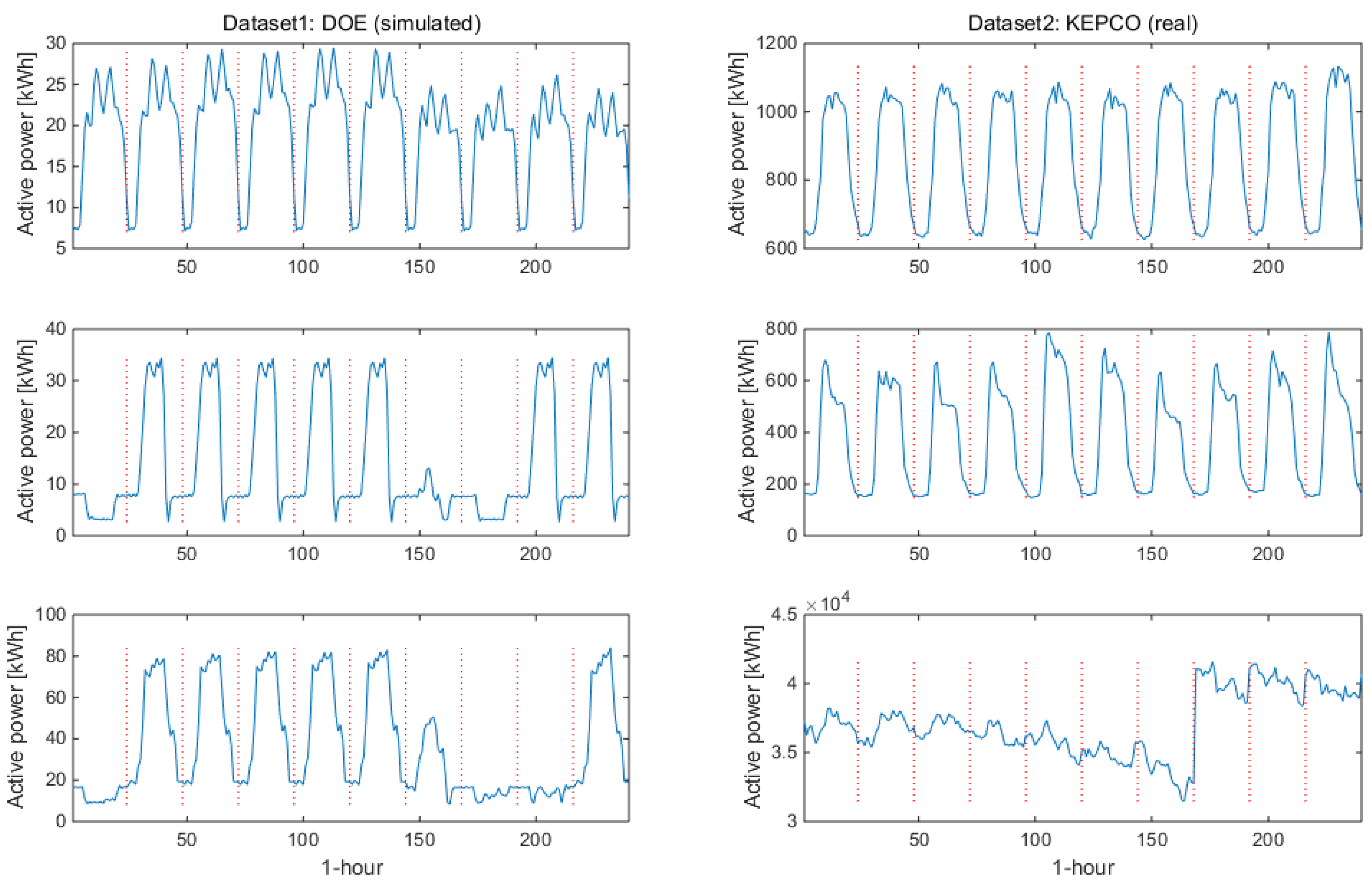
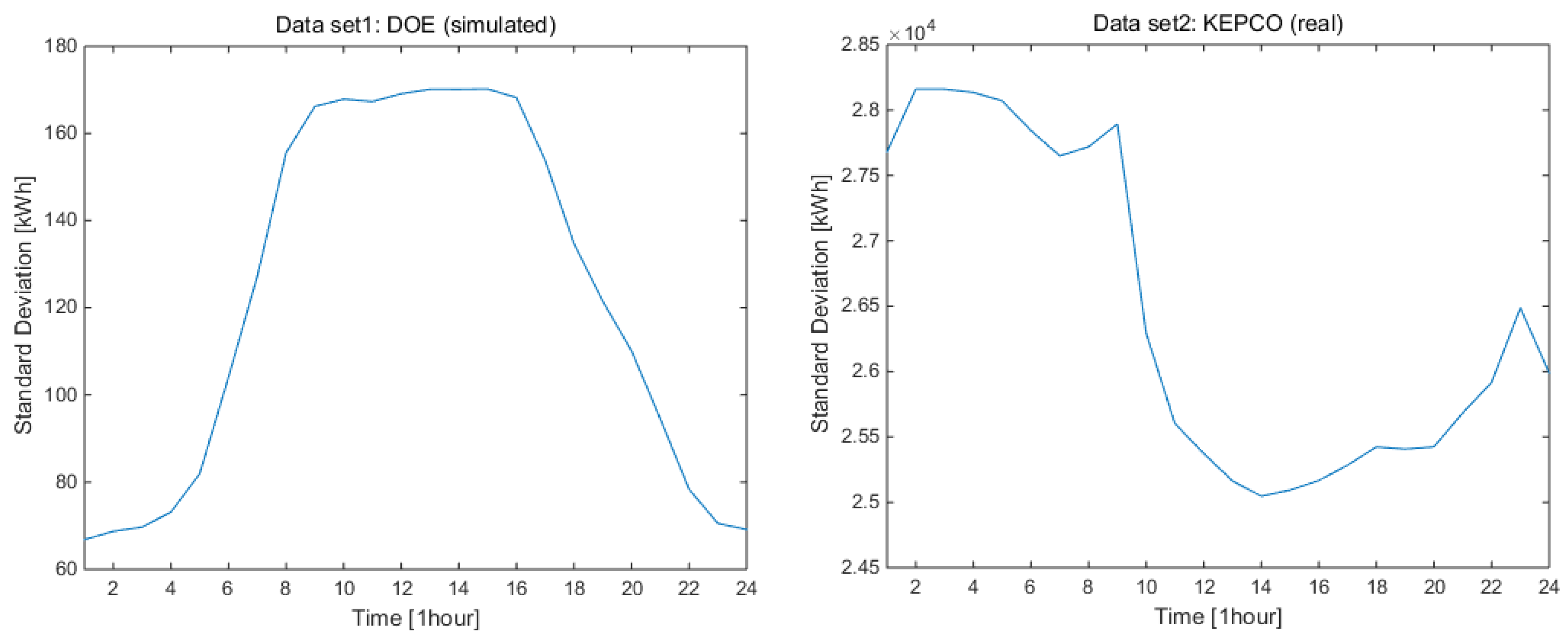
Figure 2 shows some example data from each data set. The standard deviations on each hour for both data sets are shown in Figure 3. The standard deviations of the DOE data set are much smaller than the KEPCO data set. The averages on the standard deviations of each hour are 122 kWh for DOE data set and 26,445 kWh for KEPCO data set. As the objective of this study is to extract the profiles by clustering, not assign the entire data instances into proper clusters, portions of the complete data sets are randomly selected for the performance evaluation. For both of the data sets, 10% of the data instances are used. In advance of the experiment, median filtering with a window size of 3 is applied to reduce the influence of noise on the profiles; then, the data instances are normalized.

4.3. The Result of the Performance Evaluation

The performance of clustering with SPCC distance and Euclidean distance are compared with respect to various clustering sensitivities. For Mean-Shift clustering, a hyperparameter $\alpha \in \left(0,1\right]$ is used in bandwidth control, which determines the sensitivity. The bandwidth is set to be the distance from the currently updating data instance to the kth closest data instance. The value of k is determined based on the hyperparameter $\alpha$, the ratio of selected data instance number, and the dimension of the data instances.

The bandwidth increases as $\alpha$ gets large and decreases as $\alpha$ gets small. Inversely, the clustering sensitivity increases when $\alpha$ is small and decreases when $\alpha$ is large. With high clustering sensitivity, nonparametric algorithms like Mean-Shift tend to form many small sub-clusters, which are likely to be outliers. This paper does not scope the method to handle outlying clusters, and the outliers are simply excluded for the performance evaluation. In this paper, the outlying clusters are defined to be the clusters whose data instances are less than $1\%$ of the number of the total data set.

The performance evaluation results are shown in

Table 1. $I_{SD}$ index scores of DOE (simulated) data set.

$\mathit{\alpha }$	0.1	0.2	0.3	0.4	0.5	0.6	0.7	0.8	0.9	1.0
Euclidean	$3.78\times {10}^{-3}$	$2.27\times {10}^{-3}$	$1.21\times {10}^{-3}$	$8.86\times {10}^{-4}$	$6.48\times {10}^{-4}$	$7.05\times {10}^{-4}$	$7.54\times {10}^{-4}$	$7.08\times {10}^{-4}$	$8.30\times {10}^{-4}$	$6.91\times {10}^{-4}$
SPCC	$3.55\times {10}^{-3}$	$2.24\times {10}^{-3}$	$1.14\times {10}^{-3}$	$8.68\times {10}^{-4}$	$6.34\times {10}^{-4}$	$6.91\times {10}^{-4}$	$7.43\times {10}^{-4}$	$6.63\times {10}^{-4}$	$8.21\times {10}^{-4}$	$6.81\times {10}^{-4}$

and

Table 2. $I_{SD}$ index scores of KEPCO (real) data set.

$\mathit{\alpha }$	0.1	0.2	0.3	0.4	0.5	0.6	0.7	0.8	0.9	1.0
Euclidean	$6.23\times {10}^{-3}$	$7.70\times {10}^{-3}$	$3.38\times {10}^{-3}$	$3.33\times {10}^{-3}$	$5.36\times {10}^{-3}$	$5.93\times {10}^{-3}$	$6.78\times {10}^{-3}$	$6.81\times {10}^{-3}$	$5.43\times {10}^{-3}$	$5.27\times {10}^{-3}$
SPCC	$5.58\times {10}^{-3}$	$6.57\times {10}^{-3}$	$2.67\times {10}^{-3}$	$2.64\times {10}^{-3}$	$4.04\times {10}^{-3}$	$3.76\times {10}^{-3}$	$3.31\times {10}^{-3}$	$3.49\times {10}^{-3}$	$2.82\times {10}^{-3}$	$2.74\times {10}^{-3}$

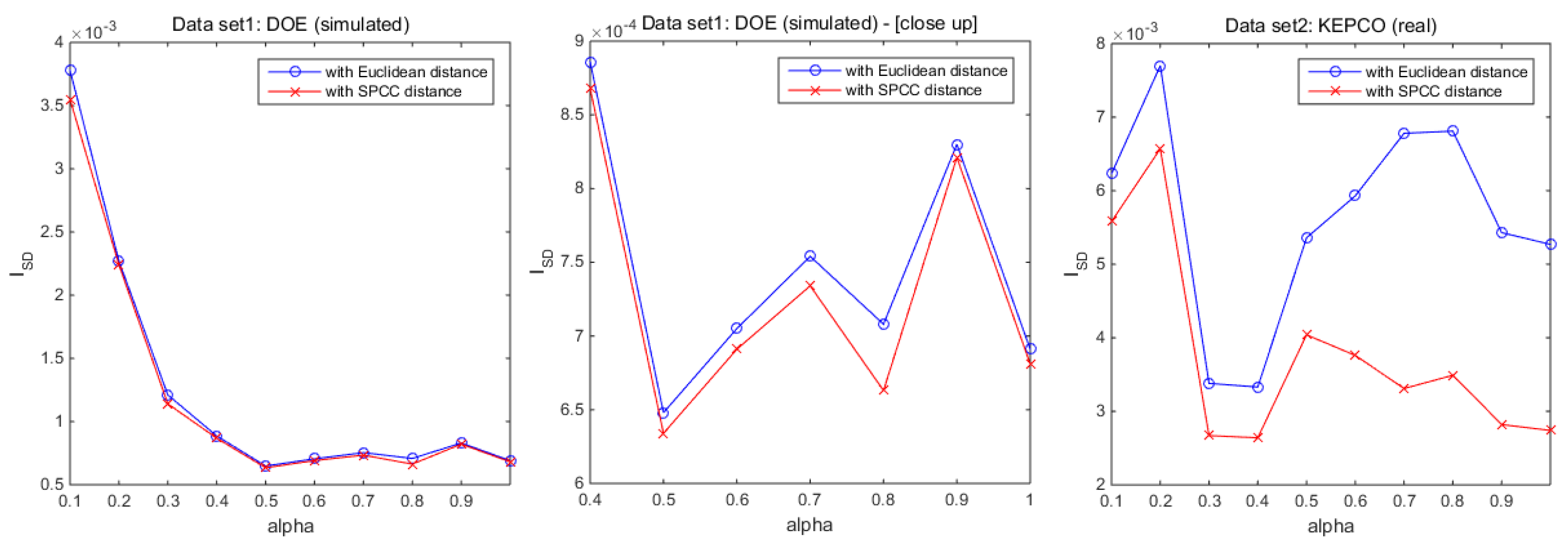
, and the results are visualized in Figure 4. The lower the $I_{SD}$ score, the better, and the graphs in Figure 4 show that the curves of the index scores with SPCC distance are under the curves of the index scores with Euclidean distance for all $\alpha$. This validates that Mean-Shift clustering with SPCC distance has shown better performance in every case compared to the clustering with Euclidean distance. 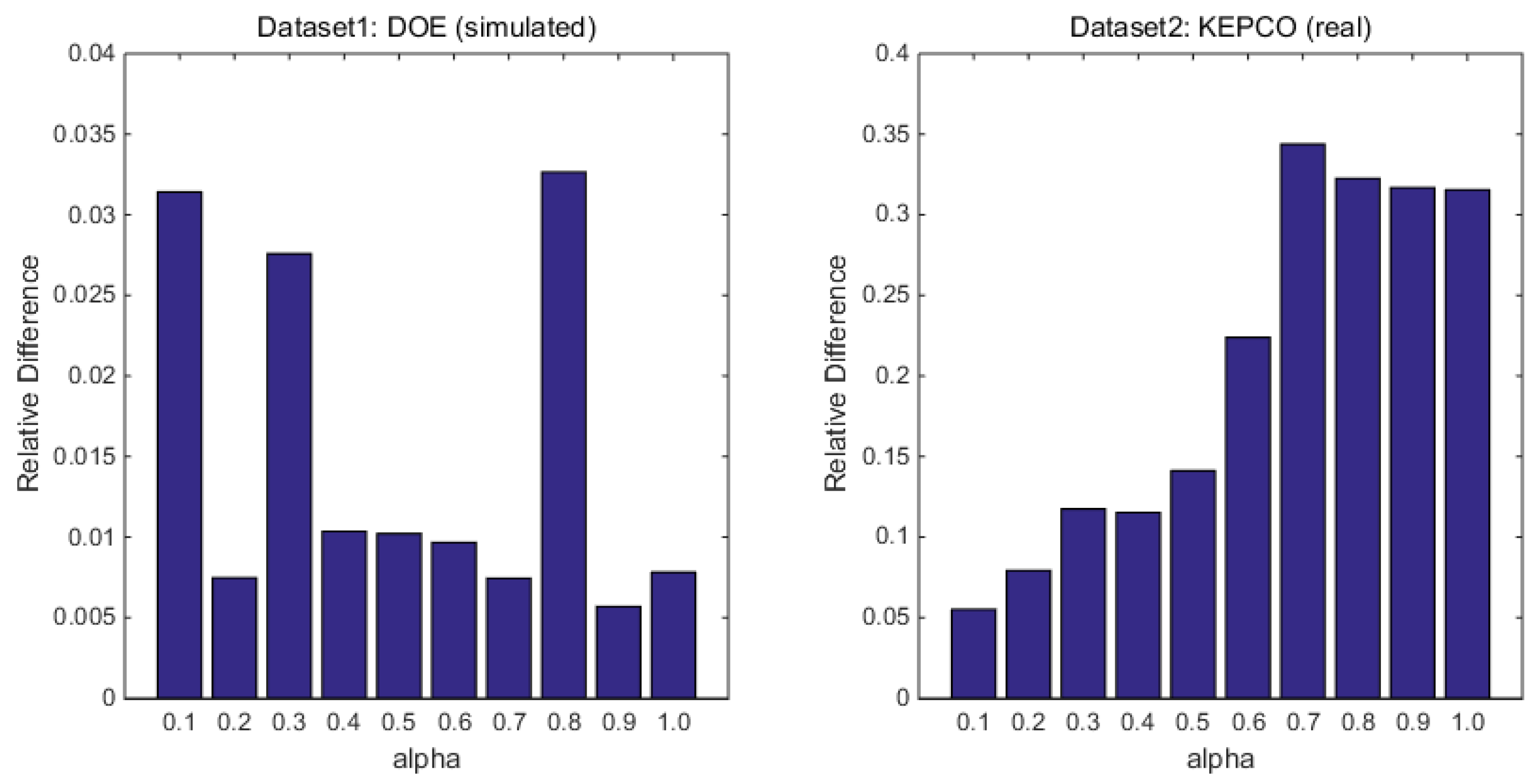The experimental results show that the most well-formed clusters are the ones clustered by SPCC distance with the hyperparameter $\alpha$ equal to 0.5 for DOE data set and 0.4 for KEPCO data set. To show the out-performance of SPCC distance more intuitively, the relative differences between $I_{SD}$ scores of the two distance methods are provided in Figure 5. The results from both the simulated and real data sets indicate the out-performance of the Mean-Shift clustering with SPCC distance over Euclidean distance regardless of the clustering sensitivity. In the case of DOE’s simulated data set, the relative difference varies from $0.55\%$ to $3.28\%$ while it varies from $5.50\%$ up to $34.39\%$ for KEPCO’s real data set. The standard deviations of the DOE data set are much smaller than the KEPCO data set. The averages on the standard deviations of each hour are 122 kWh for the DOE data set and 26,445 kWh for the KEPCO data set. This can be interpreted as the positive effects of the SPCC distance tending to stand out when the variance of electricity consumption patterns is large. Therefore, SPCC distance is preferable to Euclidean distance for real world applications.

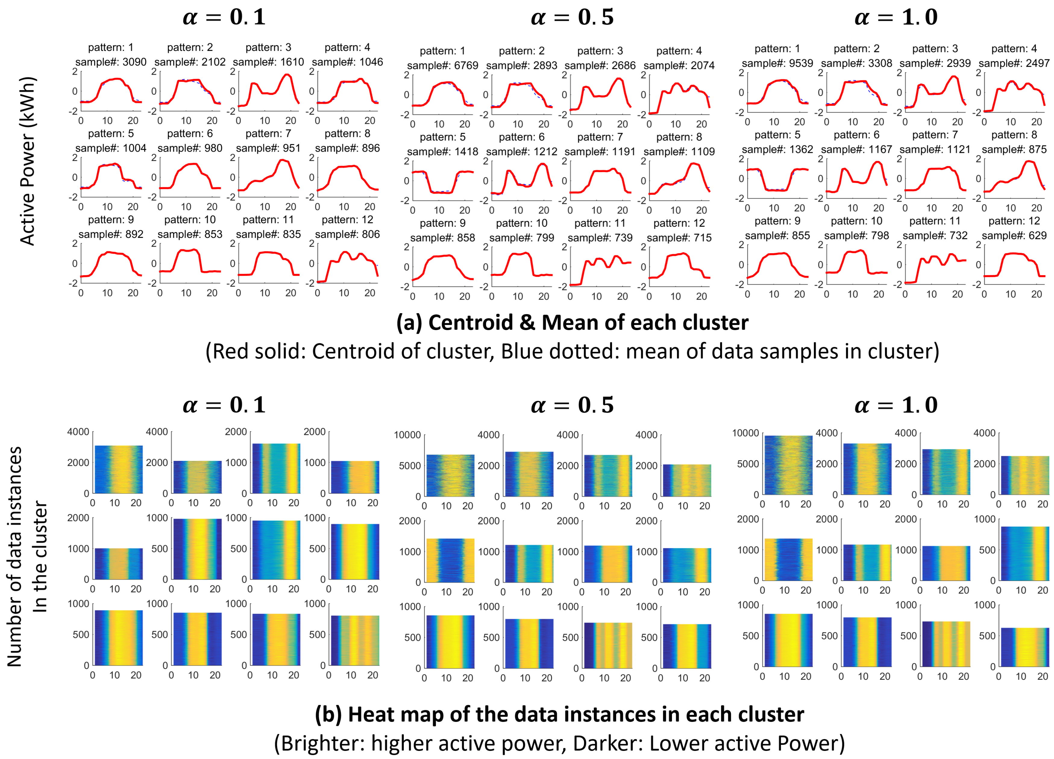
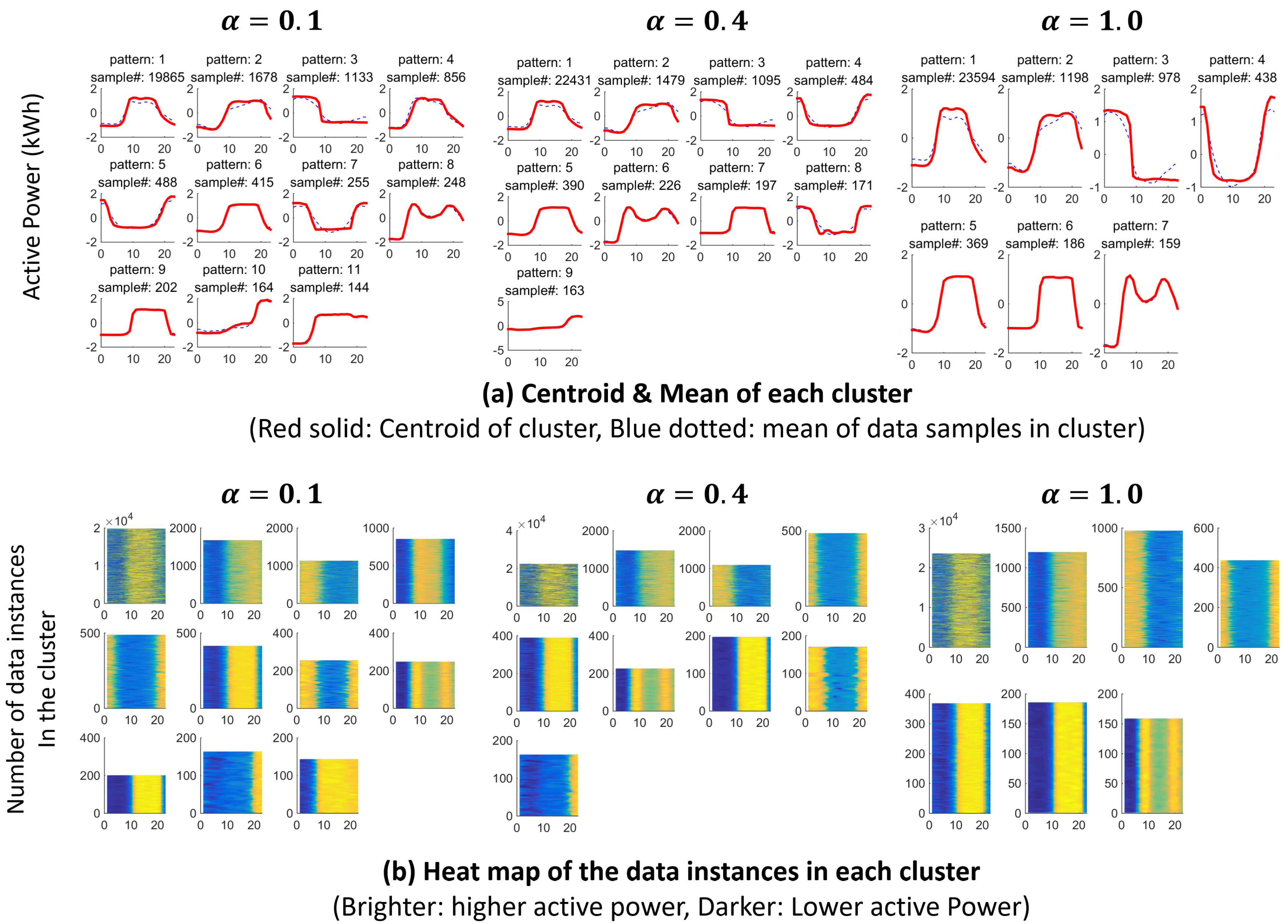
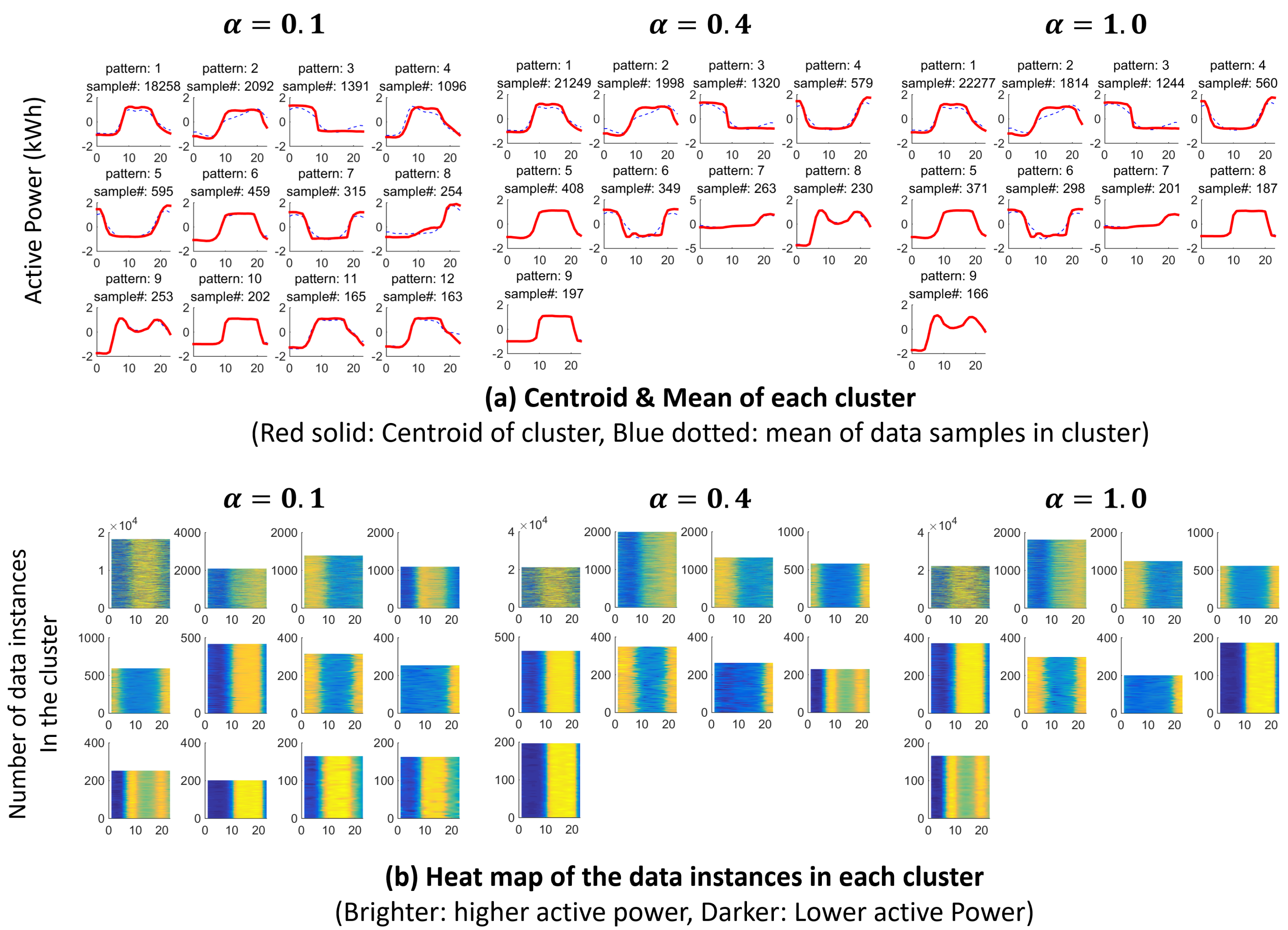
Figure 6, Figure 7, Figure 8 and Figure 9 show (a) centroids of up to the twelve largest clusters and a (b) heat-map of the data instances belonging to each cluster, respectively. (a) shows the centroids of the clusters with a red solid line and the mean of data instances belonging to the clusters with a blue dotted line. When the clusters are formed in a convex shape, the centroid and the mean tend to be similar; (b) shows the data instances’ heat-map. The yellow (light) area represents higher power load values while the blue (dark) area means power lower load values. If the color (intensity) is consistent vertically with less jitter on each hour, it indicates that the clusters are well-formed. Figure 6 is the result of a DOE data set clustered with Euclidean distance while Figure 7 with SPCC distance. Figure 8 is the result of a KEPCO data set clustered with Euclidean distance while Figure 9 with SPCC distance. For both of the data sets, cluster results with two distance measurements seem to have similar results on the centroids in their shapes, but the data instances assigned to clusters and the cluster sizes are different in each case. This indicates that distributions of data instances are interpreted differently by two distance measurements. According to the index score results, it can be concluded that SPCC distance is able to find the distribution of data instances better.

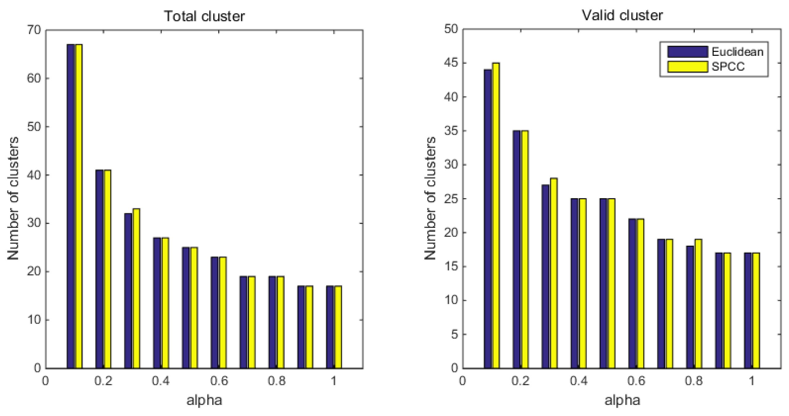
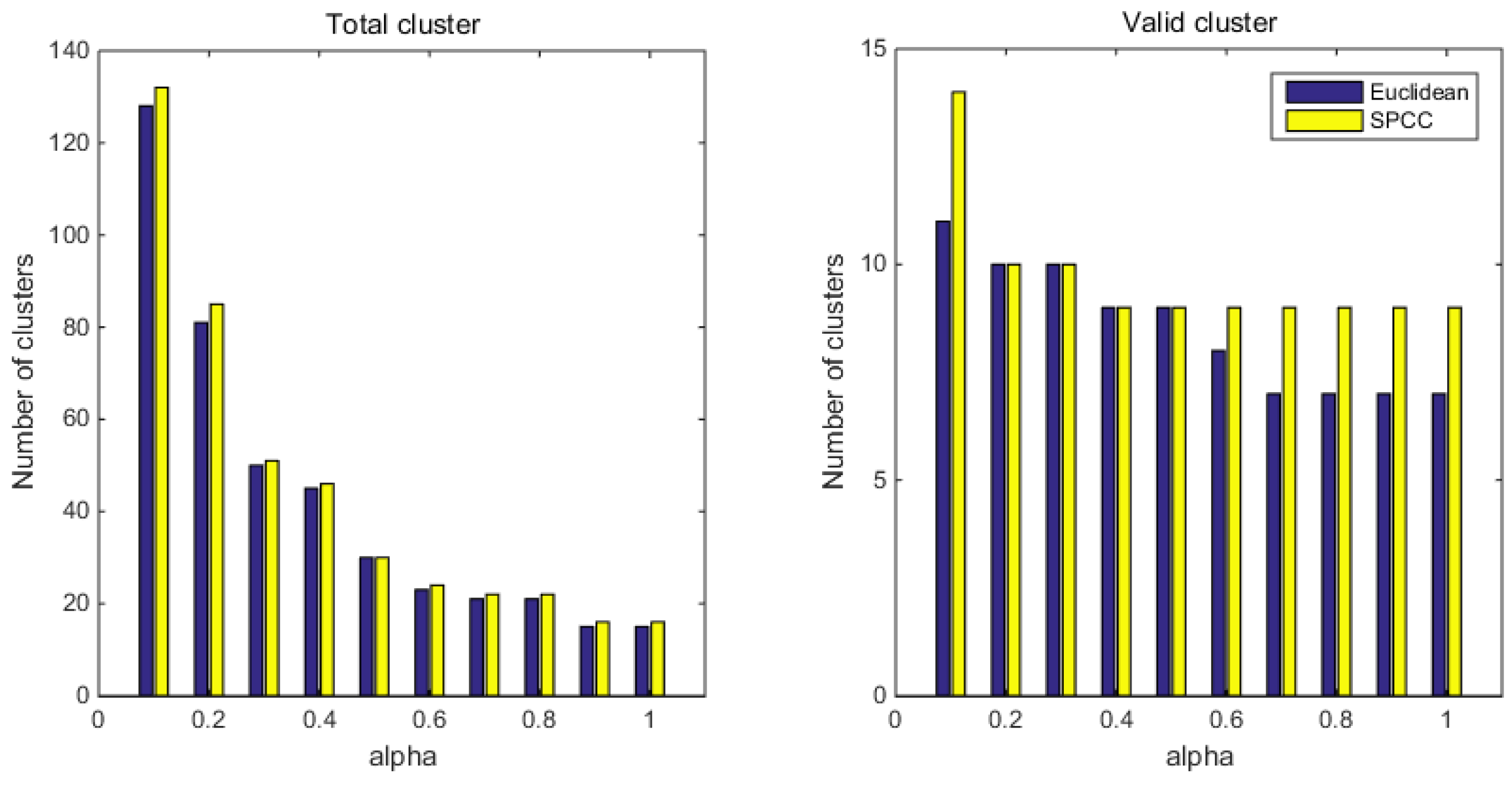
Moreover, clustering results with SPCC distance formed a greater number of clusters or at least the same compared to Euclidean distance. Figure 10 and Figure 11 show the number of clusters formed by each distance measurement. This validates that the SPCC distance based clustering is able to recognize the subtle but possibly important differences in the profiles better than Euclidean distance based clustering.

In clustering, creating clusters that are not significantly different from one another is considered to degrade the clustering quality. However, from the perspective of profiles extraction with clustering, some subtle differences can still contain important characteristics of the data sets although the clusters might have some overlaps. Accordingly, the characteristics have to be preserved to some degrees in profile extraction. In this point of view, Mean-Shift clustering with SPCC distance outperforms clustering with Euclidean distance as it extracts the typical profiles more precisely while distinguishing some subtle differences in the data clusters.

5. Discussion and Future Work

This subsection provides the implications of extracting the base load profiles cutting across various energy applications and systems. Then, related future work to deploy the proposed method into the real world systems is discussed.

As the base load profiles are extracted and validated, the profiles can be potentially used for not only further research, but also real world applications, such as load forecast, missing data imputation, differential pricing, energy system management, etc. As discussed in [32], accurate load forecasting can bring an immense amount of economic benefits. The load at a given hour depends on load values of not only the previous hours but also the same hour on previous days and weeks. According to this, the extracted base load profiles can be utilized in the load forecast. Therefore, a more precise and automated load profile extraction method will bring positive influences academically, economically, and socially. Moreover, Ref. [33] insists that one of the major challenges and opportunities arising in electric power systems is to utilize new technologies, such as sensing, computing, control, etc. The extracted load profiles can be used to summarize the large volume of data set so that can be employed by the new technologies and systems which require real-time computations and controls. Moreover, the base load profiles allow them to understand the patterns residing in the load data to discover greater values. Besides load forecast and system management, the load profiles have potentials to be applied to many research, applications, services, and systems.

For the proposed load profiles extraction method to be successfully deployed in the real world, some further analysis needs to be done. A precise and robust method to determine the sensitivity needs to be studied deeper. Outlier handling has to be accounted for. Moreover, the study on missing data imputation must be accompanied to enhance the extraction performance. On the other hand, both SPCC and Euclidean distance measurements can be utilized as well for a hybrid method in order to optimize the trade-offs between computational complexity and performance according to preference and characteristics of data sets and applications.

6. Conclusions

In this paper, a method to extract typical electricity load profiles from arbitrary data sets by clustering is discussed. This paper proposes utilizing SPCC distance for a nonparametric density-based clustering with a Mean-Shift algorithm. This method considers the electricity power load data for a day to be a single data instance, clusters the data instances based on Mean-Shift algorithm with proposed SPCC distance, and extracts centroids of the clusters as the typical load profiles of the data set. The validity of utilizing SPCC distance in Mean-Shift clustering for electricity load analysis was shown by mathematical analysis and experimental results. A density-based internal cluster quality index, $I_{SD}$, validated that the clustering with SPCC distance formed clusters better compared to the results clustered with Euclidean distance. Moreover, the proposed method to extract profiles with SPCC distance was able to recognize the profiles with subtle differences but possibly important characteristics as it detected sub-clusters better. In addition, SPCC distance based clustering with the hyperparameter, $\alpha$, equal to 0.5 and 0.4 respectively obtained the most validated results overall for both data sets. The meanings and advantages of base load extraction and the future work to deploy the proposed method into the real world applications are discussed.