A Novel Pilot Protection Principle Based on Modulus Traveling-Wave Currents for Voltage-Sourced Converter Based High Voltage Direct Current (VSC-HVDC) Transmission Lines

Abstract

Protection for transmission lines is one of crucial problems that urgently to be solved in constructing the future high-voltage and large-capacity voltage-sourced converter based high voltage direct current (VSC-HVDC) systems. In order to prevent the DC line fault from deteriorating further due to the failure of main protection, a novel pilot protection principle for VSC-HVDC transmission lines is proposed in this paper. The proposed protection principle is based on characteristics of modulus traveling-wave (TW) currents. Firstly, the protection starting-up criterion is constructed by using the absolute value of the 1-mode TW current gradient. Secondly, the fault section identification is realized by comparing the polarities of wavelet transform modulus maxima (WTMM) of 1-mode initial TW currents acquired from both terminals of the DC line. Then, the selection of fault line is actualized according to the polarity of WTMM of local 0-mode initial reverse TW current. A four-terminal VSC-based DC grid electromagnetic transient model based on the actual engineering parameters is built to assess the performance of the proposed pilot protection principle. Simulation results for different cases prove that the proposed pilot protection principle is excellent in reliability, selectivity, and robustness. Moreover, the data synchronization is not required seriously. Therefore, the proposed novel pilot protection principle can be used as a relatively perfect backup protection for VSC-HVDC transmission lines.

1. Introduction

The voltage-sourced converter based high voltage direct current (VSC-HVDC) technologies has been widely recognized as a practicable solution to implement optimal allocation, wide-area reciprocity, and flexible consumption of large-scale renewable energy over long distances [1,2]. The use of overhead transmission lines (OHLs) for power transmission is still considered to be the dominant transmission form for the future VSC-HVDC systems. However, when compared with alternating current (AC) system, serious damage to the power electronic components or a complete shutdown of the whole VSC-HVDC system will be caused by the steep rising fault current, owing to the low impedance of the short-circuit path. Moreover, temporary faults will occur with a higher probability because of the use of OHLs in unpredictable and harsh environments [3,4,5]. Consequently, protection for transmission lines is one of crucial problems that urgently to be solved in constructing the future high-voltage and large-capacity VSC-HVDC systems.

The “low inertia” characteristic of VSC-HVDC systems puts forward an extremely strict requirement on the action speed of line protection [6]. The main protection should adopt the protection principle based on single-terminal quantities [7,8,9] to obtain the fastest action speed, and therefore serious line faults can be detected and isolated as early as possible [10]. However, the main protection may be failure due to the lack of sensitivity to high impedance faults and line-terminal faults [11,12]. Therefore, in order to prevent the DC line fault from deteriorating further after the failure of the main protection, highly sensitive and selective backup protection for VSC-HVDC transmission lines should be considered.

Recently, some valuable research has been made around the backup protection for VSC-HVDC transmission lines. A novel current differential protection principle considering the frequency-dependent characteristic of cable line is proposed in [13]. The proposed protection principle can not only decrease the effect of the distributed capacitance but also improve the sensitivity of differential protection remarkably, while a larger amount of calculation and a longer time-delay are needed. Traveling-wave (TW) based differential protection schemes are proposed in [14,15]. The proposed protection principle can provide the most exact replica of the fault current, and therefore has very high reliability and selectivity. However, high sampling rate, communication speed, and the seriously synchronous current data are required. A novel pilot protection for VSC-HVDC transmission lines based on parameter identification is proposed in [16]. S-transform is utilized to extract the high-frequency component and then the sudden change value of the fault current high-frequency components is used to distinguish the internal fault. However, not only a high sampling frequency is required, but also a matching faulty pole selection is not given in the proposed method. A traveling-wave-based fault location scheme for MMC-based multi-terminal DC grids is proposed in [17]. Continuous wavelet transform (CWT) is utilized to extract and quantify the first arrival current traveling wave and then the fault location is realized with the corresponding TW characteristics. While, the amount of calculation in faulty pole identification is increased. Moreover, CWT is not easy to realize in an engineering application. A fast directional pilot protection scheme for the MMC-based MTDC grid is proposed in [18]. Features of fault voltages on both sides of the DC reactor are extracted by discrete wavelet transform, then the faulty line selection is realized with the amplitude ratio of their detail coefficients. However, the action speed will be affected by the data window of 3 ms to a certain extent.

In this paper, a novel pilot protection principle based on modulus traveling wave currents for VSC-HVDC transmission lines is proposed. Propagation characteristics of modulus TWs on DC transmission lines based on frequency-dependent model are firstly analyzed. Then the proposed novel pilot protection principle composed of protection starting-up criterion, fault section identification, and faulty line selection is realized on basis of characteristics of the modulus TW currents.

The remainder of this paper is arranged as follows. In Section 2, directional current TWs, modulus extraction and wavelet analysis theory are introduced, which are the theoretical analysis basis of the proposed pilot protection principle. Propagation characteristics of modulus TWs on DC transmission lines based on frequency-dependent model are analyzed in Section 3, the results of which is utilized to determine the decomposition scale of wavelet transform when extracting fault characteristics. In Section 4, the detail pilot protection principle is presented, including protection starting-up criterion, fault section identification and faulty line selection. Extensive simulations are conducted to evaluate the effectives of the proposed pilot protection in Section 5. Finally, some valuable conclusions are summarized in Section 6.

2. Basic Principles

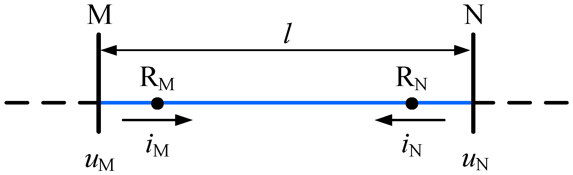
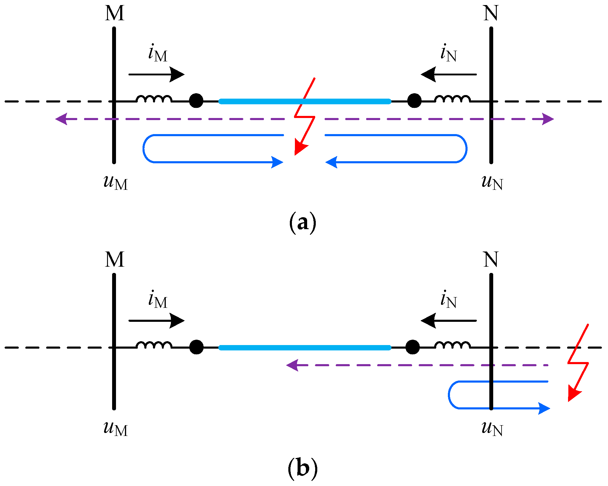
2.1. Directional Current Traveling Waves

The distributed parameter model of a uniform transmission line with a length of Δx is shown in Figure 1. The voltage u(x, t) and current i(x, t) at any position on the line are functions of distance and time [19].

Assuming that the line parameters do not vary with frequency, the voltage and current on this line satisfy the wave equations shown in Equation (1).

$$\{\begin{array}{l}-\frac{\partial u(x,t)}{\partial x}=r_{0}i(x,t)+l_0\frac{\partial i(x,t)}{\partial t}\\ -\frac{\partial i(x,t)}{\partial x}=g_{0}u(x,t)+c_0\frac{\partial u(x,t)}{\partial t}\end{array}$$

(1)

where r₀, l₀, g₀, and c₀ are the resistance, inductance, conductance, and capacitance in per unit length, respectively.

The frequency-domain form of the above wave equations can be expressed as:

$$\{\begin{array}{l}-\frac{\mathrm{d}U(x,\omega )}{\mathrm{d}x}=(r_0+j\omega l_0)I(x,\omega )\\ -\frac{\mathrm{d}I(x,\omega )}{\mathrm{d}x}=(g_0+j\omega c_0)U(x,\omega )\end{array}$$

(2)

The general solution form of Equation (2) is:

$$\{\begin{array}{l}U(x,\omega )=u_f(x,\omega )e^{-\gamma (\omega )x}+u_r(x,\omega )e^{\gamma (\omega )x}\\ I(x,\omega )=\frac{1}{Z_c(\omega )}(u_f(x,\omega )e^{-\gamma (\omega )x}-u_r(x,\omega )e^{\gamma (\omega )x})\end{array}$$

(3)

According to Equation (3), the forward voltage TW (FVTW) u_f (x, ω) and reverse voltage TW (RVTW) u_r(x, ω) can be calculated as:

$$\{\begin{array}{l}{u}_f(x,\omega )=\frac{1}{2}\left[U(x,\omega )+Z_c(\omega )I(x,\omega )\right]e^{\gamma (\omega )x}\\ u_r(x,\omega )=\frac{1}{2}\left[U(x,\omega )-Z_c(\omega )I(x,\omega )\right]e^{-\gamma (\omega )x}\end{array}$$

(4)

where Z_c(ω) and γ are the line wave impedance and the corresponding TW propagation coefficient, respectively, which can be expressed as:

$$\{\begin{array}{l}{Z}_c(\omega )=\sqrt{\frac{R+j\omega L}{G+j\omega C}}\\ \gamma (\omega )=\sqrt{(R+j\omega L)(G+j\omega C)}\end{array}$$

(5)

A uniform transmission line based on the distributed parameter model can be shown in Figure 2, the direction from bus bar to the line is defined as the reference direction for current. For convenience, the direction from bus bar M to bus bar N is defined as the reference direction for forward current TW (FCTW) at relaying point R_M and R_N, and the reference direction for reverse current TW (RCTW) is opposite.

Based on the reference direction, the voltages and currents of both the terminals satisfy boundary condition shown in Equation (6).

$$\{\begin{array}{l}{U}_M(\omega )=U(0,\omega )\\ U_N(\omega )=U(l,\omega )\\ I_M(\omega )=I(0,\omega )\\ I_N(\omega )=-I(l,\omega )\end{array}$$

(6)

Directional current TWs can be obtained by solving Equations (4) and (6) simultaneously:

$$\{\begin{array}{l}{I}_{Mf}(\omega )=0.5[U_M(\omega )/Z_c(\omega )+I_M(\omega )]\\ I_{Mr}(\omega )=0.5[U_M(\omega )/Z_c(\omega )-I_M(\omega )]\\ I_{Nf}(\omega )=0.5[U_N(\omega )/Z_c(\omega )-I_N(\omega )]\\ I_{Nr}(\omega )=0.5[U_N(\omega )/Z_c(\omega )+I_N(\omega )]\end{array}$$

(7)

where I_Mf(ω) and I_Mr(ω) are FCTW and RCTW flowing through relaying point R_M at bus bar M. I_Nf(ω) and I_Nr(ω) are FCTW and RCTW flowing through relaying point R_N at bus bar N, respectively.

2.2. Modulus Extraction

For a bipolar VSC-HVDC system, the wave equations with mutual coupling of the line are [20]:

$$\{\begin{array}{l}\frac{\partial \mathit{u}}{\partial x}=-\mathit{R}\mathit{i}-\mathit{L}\frac{\partial \mathit{i}}{\partial t}\\ \frac{\partial \mathit{i}}{\partial x}=-\mathit{G}\mathit{u}-\mathit{C}\frac{\partial \mathit{u}}{\partial t}\end{array}$$

(8)

where

$$\begin{array}{cc}\mathit{u}=\left[\begin{array}{l}{u}_p\\ u_n\end{array}\right]& \mathit{i}=\left[\begin{array}{l}{i}_p\\ i_n\end{array}\right]\\ \mathit{R}=\left[\begin{array}{cc}{R}_s& R_m\\ R_m& R_s\end{array}\right]& \mathit{L}=\left[\begin{array}{cc}{L}_s& L_m\\ L_m& L_s\end{array}\right]\\ \mathit{G}=\left[\begin{array}{cc}{G}_s& G_m\\ G_m& G_s\end{array}\right]& \mathit{C}=\left[\begin{array}{cc}{C}_s& C_m\\ C_m& C_s\end{array}\right]\end{array}$$

u_p and u_n are positive-pole and negative-pole line voltages. i_p and i_n are positive-pole and negative-pole line currents. R_s and R_m are the self-resistance and mutual-resistance. L_s and L_m are the self-inductance and mutual-inductance. G_s and G_m are the self-conductance and mutual-conductance. C_s and C_m are the self-capacitance and mutual-capacitance of the line.

For wave Equation (8), a decoupling phase-mode transform matrix can be given as:

$$\mathit{S}=\frac{1}{\sqrt{2}}\left[\begin{array}{cc}1& 1\\ -1& 1\end{array}\right]$$

(9)

By using the decoupling matrix, Equation (9) can be deduced to:

$$\{\begin{array}{l}\frac{\partial {\mathit{u}}_{\mathrm{m}}}{\partial x}=-{\mathit{S}}^{-1}\mathit{R}\mathit{S}{\mathit{i}}_{\mathrm{m}}-{\mathit{S}}^{-1}\mathit{L}\mathit{S}\frac{\partial {\mathit{i}}_{\mathrm{m}}}{\partial t}\\ \frac{\partial {\mathit{i}}_{\mathrm{m}}}{\partial x}=-{\mathit{S}}^{-1}\mathit{G}\mathit{S}{\mathit{u}}_{\mathrm{m}}-{\mathit{S}}^{-1}\mathit{C}\mathit{S}\frac{\partial {\mathit{u}}_{\mathrm{m}}}{\partial t}\end{array}$$

(10)

where

$$\begin{array}{cc}{\mathit{u}}_{\mathrm{m}}={\mathit{S}}^{-1}\mathit{u}=\left[\begin{array}{l}{u}_1\\ u_0\end{array}\right]& {\mathit{i}}_{\mathrm{m}}={\mathit{S}}^{-1}\mathit{i}=\left[\begin{array}{l}{i}_1\\ i_0\end{array}\right]\end{array}$$

$$\begin{array}{l}{\mathit{S}}^{-1}\mathit{R}\mathit{S}=\left[\begin{array}{l}{R}_1\\ R_0\end{array}\right]=\left[\begin{array}{cc}{R}_s-R_m& 0\\ 0& R_s+R_m\end{array}\right]\\ {\mathit{S}}^{-1}\mathit{L}\mathit{S}=\left[\begin{array}{l}{L}_1\\ L_0\end{array}\right]=\left[\begin{array}{cc}{L}_s-L_m& 0\\ 0& L_s+L_m\end{array}\right]\\ {\mathit{S}}^{-1}\mathit{G}\mathit{S}=\left[\begin{array}{l}{G}_1\\ G_0\end{array}\right]=\left[\begin{array}{cc}{G}_0+2G_m& 0\\ 0& G_0\end{array}\right]\\ {\mathit{S}}^{-1}\mathit{C}\mathit{S}=\left[\begin{array}{l}{C}_1\\ C_0\end{array}\right]=\left[\begin{array}{cc}{C}_0+2C_m& 0\\ 0& C_0\end{array}\right]\end{array}$$

u₁ and u₀ are 1-mode and 0-mode voltages. i₁ and i₀ are 1-mode and 0-mode currents. R_j, L_j, G_j, and C_j are j-mode (j = 0,1) resistance, inductance, conductance, and capacitance, respectively.

2.3. Wavelet Analysis Theory

Wavelet transform has been recognized as an effective tool to detect the local abrupt changes in transient signals [21,22,23], so it is very suitable for analyzing and extracting features of non-stationary high-frequency fault TW signals. Dyadic wavelet transform (DWT) is proverbially utilized to extract TW wave fronts in virtue of its significant characteristic of translation invariance with respect to time. Among the wavelet functions corresponding to the DWT, the derivative of the cubic B-spline function is symmetrical and compactly supported, which implies that perfect time and frequency resolution can be achieved [24,25].

When DWT is employed to a discrete signal f₀(n), the corresponding low-frequency approximation and high-frequency detail coefficients can be expressed as:

$$\{\begin{array}{l}{A}_{2^j}{f}_0(n)={\displaystyle \sum _k{h}_k{A}_{2^{j-1}}{f}_0(n-2^{j-1}k)}\\ W_{2^j}{f}_0(n)={\displaystyle \sum _k{g}_k{A}_{2^{j-1}}{f}_0(n-2^{j-1}k)}\end{array}$$

(11)

where $A_{2^j}{f}_0(n)$ and $W_{2^j}{f}_0(n)$ are the approximation coefficients and detail coefficients in scale 2^j. h_k and g_k are the low-pass and high-pass filter coefficients with regard to the aforementioned mother wavelet function, respectively.

When the derivative of the cubic B-spline function is chosen as the mother wavelet function, the corresponding filter coefficients h_k and g_k can be given as:

$$\{\begin{array}{l}{h}_k=\left\{0.125,0.375,0.375,0.125\right\}(k=-1,0,1,2)\\ g_k=\left\{2,-2\right\}\hspace{1em}\hspace{1em}\hspace{1em}\hspace{1em}\hspace{1em}\hspace{1em}\hspace{1em}(k=0,1)\end{array}$$

(12)

For a discrete signal containing frequencies from 0 to f_n, DWT decomposes the frequency band into two parts in half. The approximation coefficients are located in the frequency band 0 to f_n/2, and the detail coefficients are located in the frequency band f_n/2 to f_n. The decomposition can be repeated to achieve multi-resolution analysis for the input signal, as shown in Figure 3.

Wavelet transform modulus maxima (WTMM) is defined as the local maximum of the high-frequency detail coefficients. The translation invariance of DWT and singularity detection theory show that the WTMM points are one-to-one corresponding to the local abrupt changed points of the signal. Therefore, WTMM is employed to extract the polarities of fault current TW fronts in this paper.

3. Modulus Traveling-Wave Propagation Characteristics

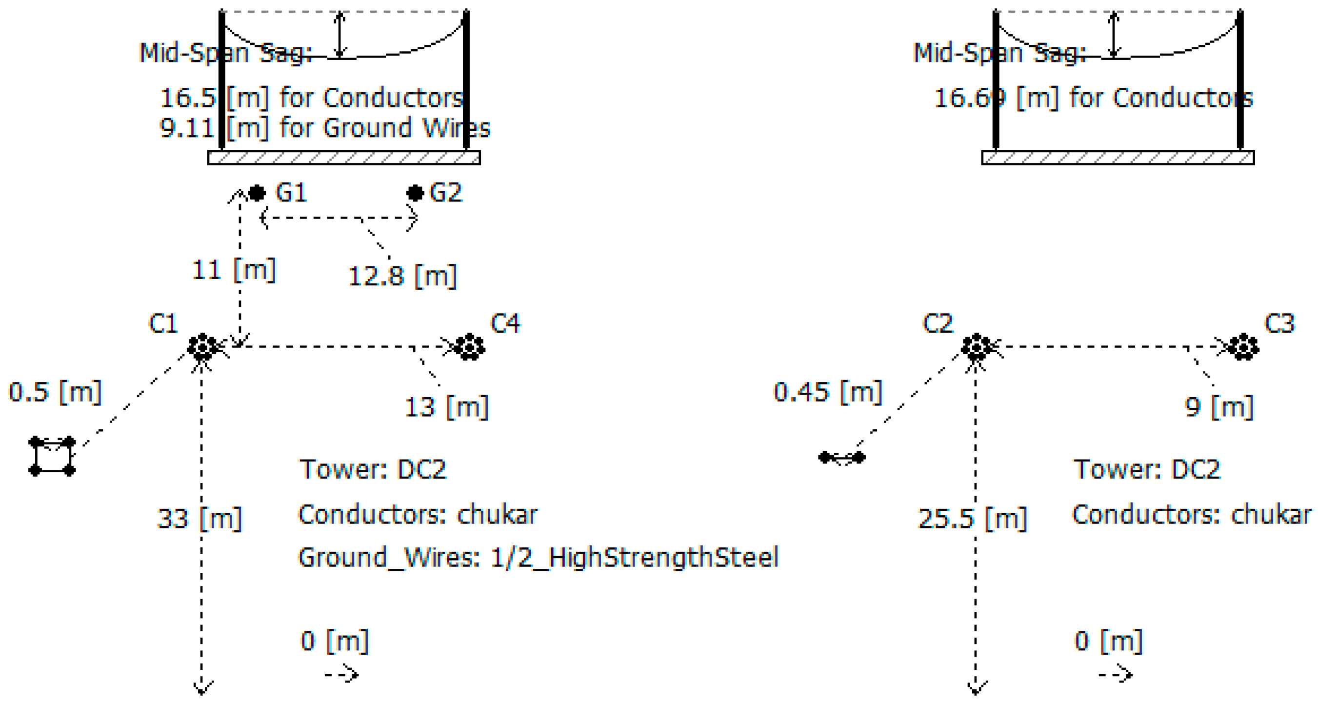
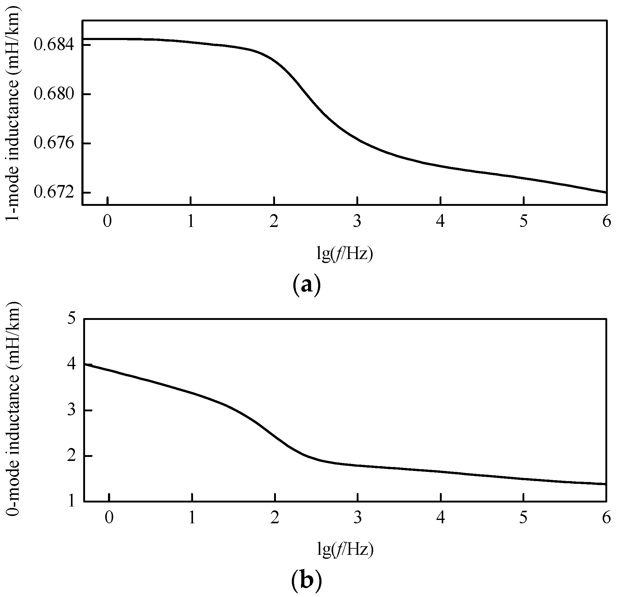
3.1. Frequency-Dependent Characteristics of DC Transmission Line Parameters

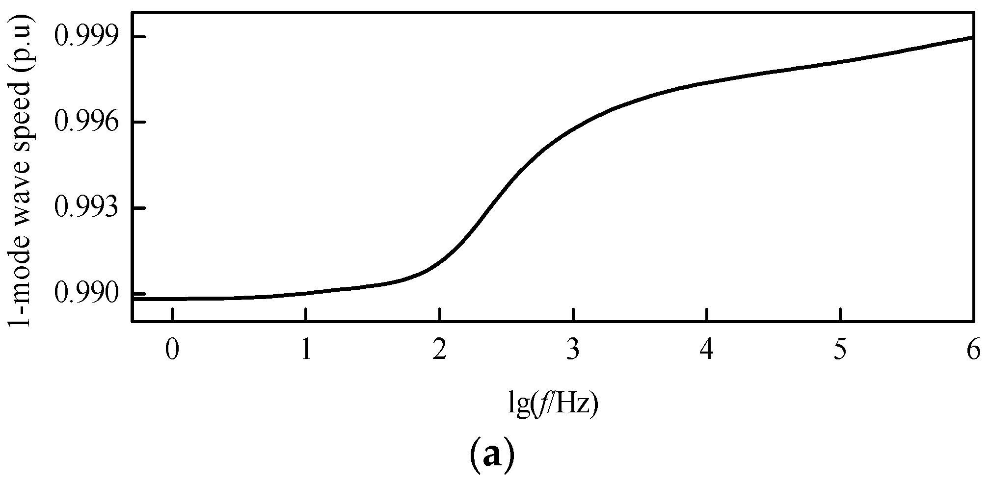
In general, the conductance of transmission line parameters can be ignored and the capacitance of which does not vary with frequency. However, the resistance and inductance vary greatly with the frequency due to the skin effect.

Configuration of a 500 kV DC transmission line is shown in Figure 4, and the modulus resistance characteristic curves after decoupling can be revealed by Figure 5. As shown in Figure 5, there is no obvious change in both the 1-mode and 0-mode resistances in per unit length within the frequency band below 10 kHz. While, with the increase of frequency, both the 1-mode and 0-mode resistances in per unit length in the frequency band above 10 kHz increase rapidly. In addition, the 0-mode resistance in per unit length is larger than the 1-mode resistance in per unit length at the same frequency.

The modulus inductance characteristic curves after decoupling can be revealed by Figure 6. In the frequency band from 1 Hz to 1 MHz, both the 1-mode and 0-mode inductances in per unit length decrease with the increase of frequency. The 1-mode inductance is only slightly reduced, while the 0-mode inductance decreases greatly. Besides, the 0-mode inductance in per unit length is larger than the 1-mode inductance in per unit length at the same frequency.

3.2. Wave Impedance

According to Equation (5), the frequency-domain form of wave impedance can be expressed as:

$$Z_c(\omega )=\sqrt{\frac{R(\omega )+j\omega L(\omega )}{G(\omega )+j\omega C(\omega )}}$$

(13)

Based on the frequency-dependent characteristics of DC transmission line parameters that are mentioned above, the modulus wave impedance characteristic curves after decoupling can be revealed by Figure 7. In the frequency band from 1 Hz to 1 MHz, the 1-mode wave impedance is approximately constant, while the 0-mode wave impedance varies greatly.

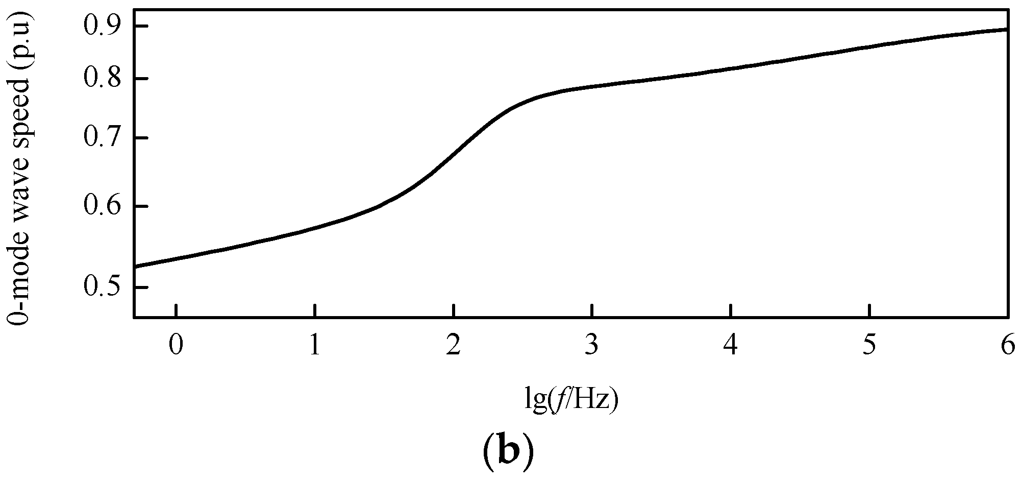
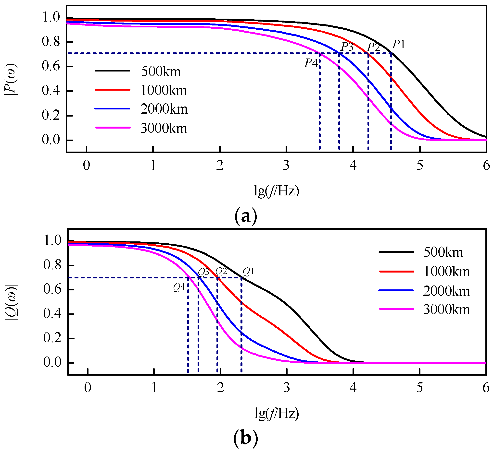
3.3. Propagation Functions

The frequency-domain form of TW wave speed can be expressed as:

$$v(\omega )=\frac{1}{\sqrt{L(\omega )C}}$$

(14)

Based on the frequency-dependent characteristics of the DC transmission line parameters mentioned above, the modulus TW wave speed characteristic curves after decoupling can be revealed by Figure 8. In the frequency band from 1 Hz to 1 MHz, the wave speed of the 1-mode TW is close to that of light in a vacuum, while the wave speed of the 0-mode TW is obviously smaller than that of the 1-mode TW.

According to Equation (5), the frequency-domain form of TW propagation coefficient can be expressed as:

$$\gamma (\omega )=\sqrt{\left[R(\omega )+j\omega L(\omega )\right]\left[G(\omega )+j\omega C(\omega )\right]}$$

(15)

The TW propagation function can be defined as:

$$\eta (\omega )={\mathrm{e}}^{-\gamma (\omega )x}$$

(16)

where x is the TW propagation distance.

The characteristic curves of the modulus TW propagation functions after decoupling at different distances can be shown in Figure 9. At the same frequency, the longer the propagation distance, the more serious the TW attenuation. At the same propagation distance, the higher the TW frequency, the more serious the TW attenuation. Besides, at the same frequency and propagation distance, the attenuation of 0-mode TWs are more serious.

The cut-off frequencies for which the modulus TW attenuating to 0.7 times of its original value are shown in

Table 1. Cut-off frequencies of modulus TWs with different distances.

Distances/km	Cut-off Frequencies
	P(ω)/kHz	Q(ω)/Hz
200	128.8	1380.4
500	39.8	213.8
1000	16.9	89.1
2000	6.3	47.9
3000	3.2	33.88

. At the same propagation distance, the cut-off frequency of 1-mode TW is much higher than that of 0-mode TW. Moreover, the cut-off frequencies of modulus TWs gradually decrease with the increase of propagation distance. On basis of the cut-off frequencies of modulus TWs at different distances that are shown in Table 1, the scale of wavelet transform can be determined for a signal with known sampling frequency.

4. Protection Scheme

As shown in Figure 10, when a fault f occurs on the DC transmission line, according to the TW theory, it is equivalent to superimposing an additional DC voltage source u_f (t) at the fault point. With the influence of the additional DC voltage source, high-frequency voltage and current TWs are generated and hereafter propagate along the DC transmission line from the fault point to both terminals.

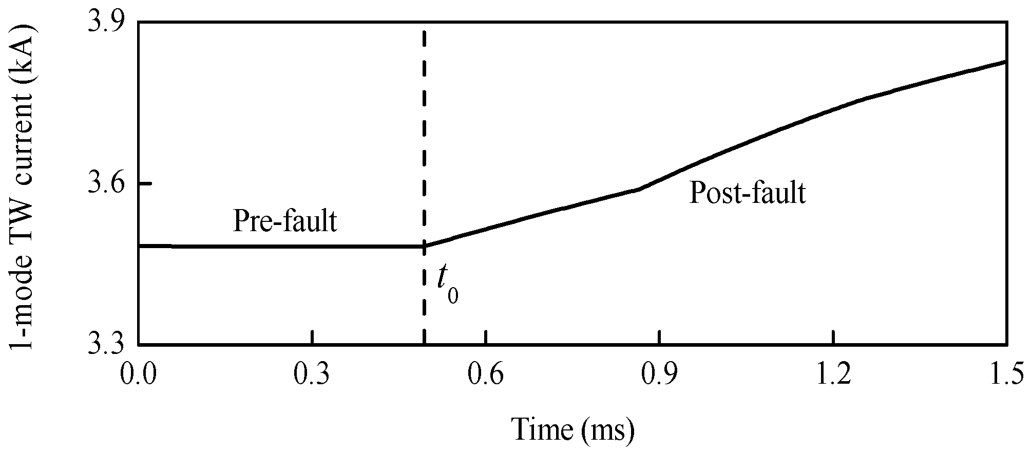
4.1. Starting-Up Element

Define the absolute value of 1-mode TW current gradient as:

$$d{i}_1(k)=\left|\frac{i_1(k)-i_1(k-1)}{\Delta t}\right|$$

(17)

where i₁(k) denotes the 1-mode TW current data at this moment, and Δt is the sampling time interval.

When there is no fault on the line, the fluctuation of 1-mode TW current i₁ is small when considering the measurement error, and therefore the absolute value of its gradient di₁ is also small correspondingly. However, once a fault occurs on the line, the 1-mode TW current i₁ will change drastically, and as a result the absolute value of its gradient di₁ increases rapidly. Consequently, the protection starting-up criterion can be set as:

$$d{i}_1(k)>{\Delta }_1$$

(18)

where Δ₁ is the threshold value of the starting-up criterion, which should be greater the normal operating maximum value of di₁(k).

To ensure the reliability, if two consecutive values di₁(k) and di₁(k + 1) exceed the threshold value Δ₁, a starting-up signal will be given out.

4.2. Fault Section Identification

In general, DC reactors are installed at both terminals of the line in VSC-HVDC systems. The DC reactors can not only limit the development of fault currents, but also provide natural boundary conditions for line protection. When a fault occurs on the line, the refraction and reflection will occur at the DC reactor for the generated fault TWs. As shown in Figure 11, the purple dotted line denotes the refracted TW, and the blue solid is the reflected TW. Because of the discontinuous wave impedance presented by the DC reactor, an abrupt change will occur when the TW propagate along the transmission line to the DC reactor. When an internal fault occurs for the line MN, the abrupt change polarities of initial 1-mode TW currents detected at both terminals of the line MN are the same. However, when an external fault occurs for the line MN, the abrupt change polarities of initial 1-mode TW currents detected at both terminals of the line MN are opposite.

Supposing that WTMM(i_M1) and WTMM(i_N1) are the WTMMs of the initial 1-mode TW currents detected at terminal M and terminal N, respectively. The result of sign function 1 denotes that the abrupt change polarity of the initial 1-mode TW current is positive and -1 represents a negative abrupt change polarity. According to the abrupt change polarities of initial 1-mode TW currents detected at both terminals of the line, fault section identification criterion can be designed.

If

$$sign\left[\mathrm{WTMM}\left(i_{\mathrm{M}1}\right)\right]\times sign\left[\mathrm{WTMM}\left(i_{\mathrm{N}1}\right)\right]=1$$

(19)

is satisfied, the fault can be identified as an internal fault for the line. Otherwise, the fault is identified as an external fault.

4.3. Faulty Line Selection

For a bipolar VSC-HVDC system, when a positive pole-to-ground short-circuit fault occurs, the fault superimposed network can be shown in Figure 12.

According to the boundary conditions, the following equations can be given as:

$$\{\begin{array}{l}{u}_{\mathrm{p}}=u_{\mathrm{pf}}-2i_{\mathrm{p}}{R}_{\mathrm{f}}\\ u_{\mathrm{pf}}=-U_{\mathrm{dc}}\\ i_{\mathrm{n}}=0\end{array}$$

(20)

where u_pf is the additional DC voltage source, and R_f denotes the fault transition resistance.

Substituting the modulus resistance into Equation (20), the initial TW voltages for both poles can be derived as:

$$\{\begin{array}{c}{u}_{\mathrm{p}}=-\frac{U_{\mathrm{dc}}(Z_0+Z_1)}{Z_0+Z_1+4R_{\mathrm{f}}}\\ u_{\mathrm{n}}=-\frac{U_{\mathrm{dc}}(Z_0-Z_1)}{Z_0+Z_1+4R_{\mathrm{f}}}\end{array}$$

(21)

Appling the phase-mode transform matrix shown in Equations (9)–(21), the initial modulus TW voltages can be given as:

$$\{\begin{array}{c}{u}_1=-\frac{\sqrt{2}{U}_{\mathrm{dc}}{Z}_1}{Z_0+Z_1+4R_{\mathrm{f}}}\\ u_0=-\frac{\sqrt{2}{U}_{\mathrm{dc}}{Z}_0}{Z_0+Z_1+4R_{\mathrm{f}}}\end{array}$$

(22)

Furthermore, the corresponding initial modulus TW currents can be obtained:

$$\{\begin{array}{c}{i}_1=-\frac{\sqrt{2}{U}_{\mathrm{dc}}}{Z_0+Z_1+4R_{\mathrm{f}}}\\ i_0=-\frac{\sqrt{2}{U}_{\mathrm{dc}}}{Z_0+Z_1+4R_{\mathrm{f}}}\end{array}$$

(23)

where i₁ is the 1-mode TW current, and i₀ denotes the 0-mode TW current.

In the same manner, when a negative pole-to-ground short-circuit fault occurs, the corresponding initial modulus TW currents can be given as:

$$\{\begin{array}{l}{i}_1=-\frac{\sqrt{2}{U}_{\mathrm{dc}}}{Z_0+Z_1+4R_{\mathrm{f}}}\\ i_0=\frac{\sqrt{2}{U}_{\mathrm{dc}}}{Z_0+Z_1+4R_{\mathrm{f}}}\end{array}$$

(24)

Similarly, for a pole-to-pole short-circuit fault, the initial modulus TW can be expressed as:

$$\{\begin{array}{l}{i}_1=-\frac{\sqrt{2}{U}_{\mathrm{dc}}}{Z_1+R_f}\\ i_0=0\end{array}$$

(25)

Based on the theoretical analysis mentioned above, the faulty line selection criterion can be designed as:

$$f=\{\begin{array}{l}\mathrm{positive}\mathrm{pole}-\mathrm{to}-\mathrm{ground}\mathrm{fault},\mathrm{WTMM}\left(i_{r0}\right)<-{\Delta }_2\\ \mathrm{negative}\mathrm{pole}-\mathrm{to}-\mathrm{ground}\mathrm{fault},\mathrm{WTMM}\left(i_{r0}\right)>{\Delta }_2\\ \mathrm{pole}-\mathrm{to}-\mathrm{pole}\mathrm{fault},\hspace{1em}\hspace{1em}\hspace{1em}\hspace{1em}\hspace{1em}\hspace{1em}\hspace{1em}\mathrm{others}\end{array}$$

(26)

where i_r0 is the 0-mode reverse TW current, and Δ₂ is the threshold value of the faulty line selection criterion.

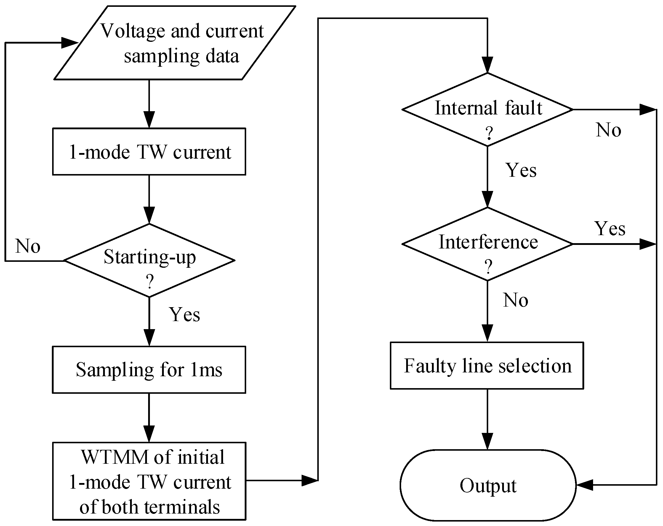
4.4. Flow Chart of Protection Scheme

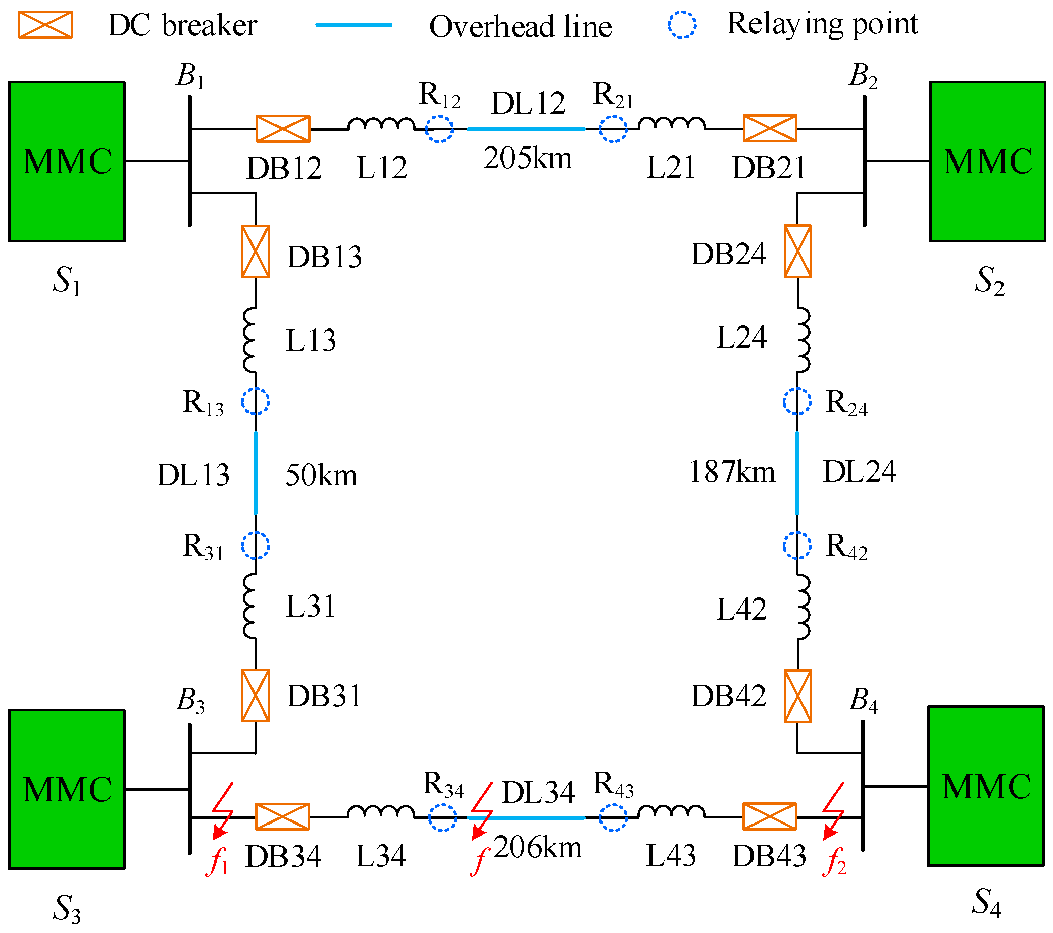
The flow chart of the protection scheme is shown in Figure 13. The voltage and current data of positive-pole and negative-pole lines are sampled and stored, and the 1-mode TW current is extracted in real time. If the starting-up condition is satisfied, data will still be sampled for 1 ms. With the data 0.5 ms before starting-up, the data of 1.5 ms data window is constituted. Then the phase-mode transform is employed and the directional 1-mode and 0-mode TW currents are calculated. Thereafter, wavelet transform is implemented to extract the WTMMs of the initial directional 1-mode and 0-mode TW currents. Next, WTMMs of the initial directional 1-mode TW currents are exchanged with the other terminal. If an internal fault is determined, according to Equation (19), then the interference identification is also needed prevent the protection from malfunction. Finally, for an internal fault, faulty line selection on the basis of Equation (26) will be executed for tripping.

5. Simulations

In order to verify the validity of the proposed protection principle, an electromagnetic transient simulation model of ±500 kV four-terminal bipolar VSC-based DC grid shown in Figure 14 is established in PSCAD/EMTDC. The DC voltage of station S₂ and the active power of other stations are the reference values for their corresponding control objects. The frequency-dependent transmission line of which the configuration is shown in Figure 4 is utilized here and the sampling frequency is 200 kHz.

Without a loss of generality, research around the line DL34 is conducted in this paper. For convenience, faults occurring on the line DL34 are internal faults, while faults occurring on other positions are defined as external faults. Moreover, based on the cut-off frequencies of modulus TWs at different distances shown in Table 1, the initial WTMM in scale 2⁴ (7.813–15.625 kHz) is extracted for fault characteristic analysis.

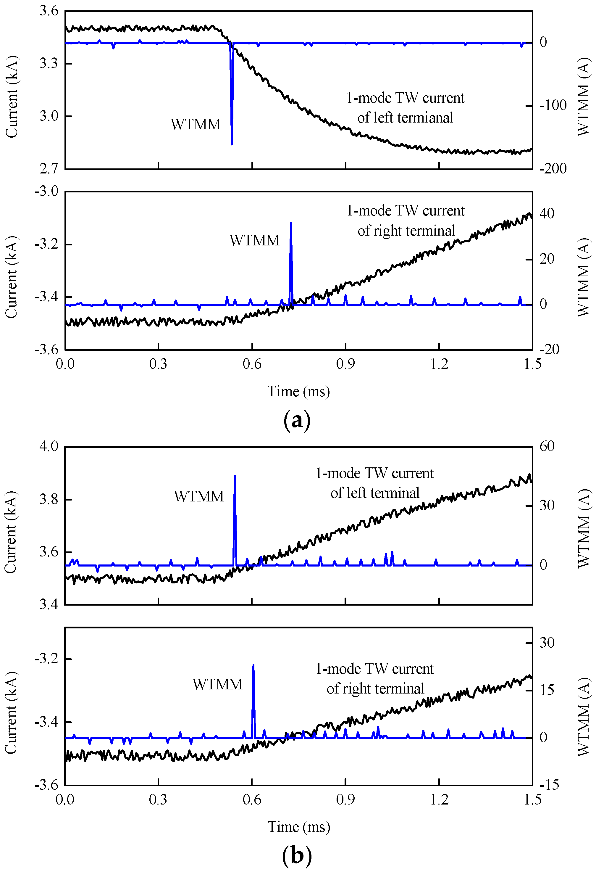
5.1. Performance of the Starting-Up Element

A positive pole-to-ground fault with 300 Ω transition resistance is set at 205.5 km away from station S₃, and the corresponding time-domain waveform of 1-mode TW current that is detected by R₃₄ is shown in Figure 15. Before the fault, the amplitude of 1-mode TW current has no obvious change. However, that of the 1-mode TW current increases rapidly after the fault.

Results of the protection starting-up element at different distances and different transition resistances is shown in

Table 2. Result of the protection starting-up element.

Distance/km	Resistance/Ω	di1
		di1(k − 1)	di1(k)	di1(k + 1)
0.5	0	3.71	863	842
	100	3.76	524	420
	200	3.83	378	309
	300	3.79	297	255
75	0	3.97	635	932
	100	3.39	386	569
	200	3.29	278	410
	300	3.18	218	320
150	0	3.34	533	893
	100	3.53	319	538
	200	3.45	226	383
	300	3.35	261	300
205.5	0	3.59	812	1012
	100	3.88	523	748
	200	3.77	385	602
	300	3.81	305	503

. Before the fault, the absolute value of the 1-mode TW current gradient is small. However, that of the 1-mode TW current gradient is much larger after the fault. Therefore, the performance of the designed protection starting-up element is reliable.

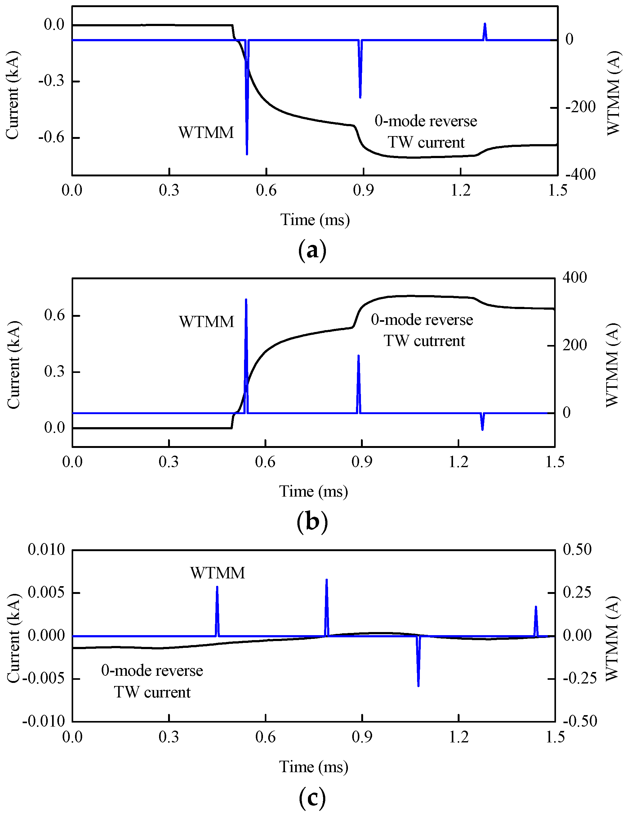
5.2. Performance of Fault Section Identification

As shown in Figure 14, metallic external positive pole-to-ground faults f₁ and f₂ are set on the lines between bus bars and DBs, and internal positive pole-to-ground faults with different transition resistances are set at 205.5 km away from station S₃. According to results that are shown in Figure 16 and

Table 3. WTMMs of 1-mode TW currents.

Location	Resistances/Ω	WTMM(i1)/A		Result
		S3 Side	S4 Side
f1	0	−165.5	37.29	External fault
f2	0	56.67	−171.5
DL34	0	82.87	43.17	Internal fault
	100	60.84	31.69
	200	48.2	25.11
	300	40.01	20.87

, the WTMMs of 1-mode TW currents at both terminals are the same for the internal fault, while those are opposite for the external fault. As a result, it is can be concluded that the performance for fault section identification is accurate and reliable for external faults nearby and internal faults with transition resistance of at least 300 Ω.

5.3. Performance of Faulty Line Selection

5.3.1. Different Fault Types

Three typical faults, namely positive pole-to-ground fault, negative pole-to-ground fault, and pole-to-pole fault are simulated to test the performance of the proposed protection. These faults with 200 Ω transition resistance are set at 150 km away from station S₃ respectively. As shown in Figure 17, WTMMs of the 0-mode initial reverse TW current for the positive pole-to-ground fault is a negative value. However, that for the negative pole-to-ground fault is a positive value. Moreover, that for the pole-to-pole fault is 0 when considering measurement error.

5.3.2. Different Transition Resistances

The same three typical faults with different transition resistances are set at 150 km away from station S₃ respectively. As shown in

Table 4. WTMMs of 0-mode initial reverse TW current under different fault resistances.

Types	Resistance/Ω	WTMM(ir0)/A	Result
1	0	−761.08	Positive pole-to-ground fault
	100	−467.51
	200	−337.33
	300	−263.84
2	0	761.24	Negative pole-to-ground fault
	100	467.59
	200	337.38
	300	263.88
3	0	0.341	Pole-to-pole fault
	100	0.328
	200	0.328
	300	0.329

, WTMMs of the 0-mode initial reverse TW current for positive pole-to-ground faults are always negative. However, those for negative pole-to-ground faults are always positive. Moreover, those for pole-to-pole faults are always 0 when considering measurement error.

5.3.3. Different Fault Distances

The same three typical faults are set at 0.5 km, 75 km, 150 km, and 205.5 km away from station S₃, respectively. The results at different fault distances are shown in

Table 5. WTMMs of 0-mode initial reverse TW current under different fault distances.

Types	Distances/km	WTMM(ir0)/A	Result
1	0.5	−424.4	Positive pole-to-ground fault
	75	−395.2
	150	−263.8
	205.5	−270.2
2	0.5	425.9	Negative pole-to-ground fault
	75	396.8
	150	263.9
	205.5	270.6
3	0.5	0.28	Pole-to-pole fault
	75	0.32
	150	0.26
	205.5	−0.35

. As expected, WTMMs of the 0-mode initial reverse TW current are always negative for positive pole-to-ground faults. While, those are always positive for negative pole-to-ground faults. Moreover, those are always 0 for pole-to-pole faults considering measurement error.

5.4. Performance Under Noise Disturbance

5.4.1. Fault Section Identification Under Noise Disturbance

Metallic external positive pole-to-ground fault f₁ is set on the line between bus bar B₃ and DB34, and a positive pole-to-ground fault with 300 Ω transition resistance is set at 205.5 km away from station S₃, respectively. 20dB Gauss white noise is added into the 1-mode TW currents that were acquired by R₃₄ and R₄₃, respectively. As shown in Figure 18, WTMMs of 1-mode TW currents at both terminals are opposite for the external fault, and those are still the same for the internal fault.

5.4.2. Faulty Line Selection Under Noise Disturbance

Under the same internal fault, 20 dB Gauss white noise is added into the 0-mode reverse TW current collected by R₃₄. As shown in Figure 19, WTMM of the 0-mode initial reverse TW current is still a larger negative value, which indicates that an internal positive pole-to-ground fault occurs on the line.

6. Conclusions

The paper proposes a novel pilot protection principle for VSC-HVDC transmission lines based on modulus TW currents. The absolute value of the 1-mode TW current gradient is constructed for protection starting-up element. The wavelet transform is employed to extract the WTMMs of modulus TW currents. The fault section identification is realized by comparing the polarities of WTMMs of 1-mode initial TW currents acquired from both terminals of the DC line. The polarity of WTMM of local 0-mode initial reverse traveling-wave current is utilized for faulty line selection. The simulation results prove the excellent performance of the proposed protection under different conditions. Moreover, the requirement of protection selectivity and sensitivity is satisfied, and the data synchronization is not required seriously. Therefore, the proposed novel pilot protection principle can be used as a relatively perfect backup protection for VSC-HVDC transmission lines.

The sequential coordination between the main protection and backup protection for VSC-HVDC transmission lines will be conducted in the future research.

References

1. Flourentzou, N.; Agelidis, V.G.; Demetriades, G.D. VSC-based HVDC power transmission systems: An overview. IEEE Trans. Power Electron. 2009, 24, 592–602. [Google Scholar] [CrossRef]
2. Nami, A.; Liang, J.; Dijkhuizen, F.; Demetriades, G.D. Modular multilevel converters for HVDC applications: Review on converter cells and functionalities. IEEE Trans. Power Electron. 2015, 30, 18–36. [Google Scholar] [CrossRef]
3. Liu, J.; Tai, N.; Fan, C. Transient-voltage-based protection scheme for DC line faults in the multiterminal VSC-HVDC system. IEEE Trans. Power Deliv. 2017, 32, 1483–1494. [Google Scholar] [CrossRef]
4. Li, S.; Chen, W.; Yin, X.; Chen, D. Protection scheme for VSC-HVDC transmission lines based on transverse differential current. IET Gener. Transm. Dist. 2017, 11, 2805–2813. [Google Scholar] [CrossRef]
5. Li, X.; Song, Q.; Liu, W.; Rao, H.; Xu, S.; Li, L. Protection of nonpermanent faults on DC overhead lines in MMC-based HVDC systems. IEEE Trans. Power Deliv. 2013, 28, 483–490. [Google Scholar] [CrossRef]
6. Xue, S.; Lian, J.; Qi, J.; Fan, B. Pole-to-ground fault analysis and fast protection scheme for HVDC based on overhead transmission lines. Energies 2017, 10, 1059. [Google Scholar] [CrossRef]
7. Zhang, B.; Zhang, S.; You, M.; Cao, R. Research on transient-based protection for HVDC lines. Power Syst. Prot. Control 2010, 38, 18–23. (In Chinese) [Google Scholar]
8. Zhang, M.; He, J.; Luo, G.; Wang, X. Local information-based fault location method for multi-terminal flexible DC grid. Electr. Power Autom. Equip. 2018, 38, 155–161. (In Chinese) [Google Scholar]
9. Yu, X.; Xiao, L.; Lin, L.; Qiu, Q.; Zhang, Z. Single-ended Fast Fault Detection Scheme for MMC-based HVDC. High Volt. Eng. 2018, 44, 440–447. (In Chinese) [Google Scholar]
10. Dong, X.; Tang, L.; Shi, S.; Qiu, Y.; Kong, M.; Pang, H. Configuration scheme of transmission line protection for flexible HVDC grid. Power Syst. Technol. 2018, 42, 1752–1759. (In Chinese) [Google Scholar]
11. Gibo, N.; Takenaka, K.; Verma, S.C.; Sugimoto, S.; Ogawa, S. Protection scheme of voltage sourced converters based HVDC system under DC fault. IEEE/PES Transm. Distrib. Conf. Exhib. 2002, 2, 1320–1325. [Google Scholar]
12. Xing, L.; Chen, Q.; Gao, Z.; Fu, Z. A new protection principle for HVDC transmission lines based on fault component of voltage and current. In Proceedings of the 2011 IEEE Power and Energy Society General Meeting, Detroit, MI, USA, 24–29 July 2011; pp. 1–6. [Google Scholar]
13. Song, G.; Cai, X.; Gao, S.; Suonan, J.; Li, G. Novel current differential protection principle of VSC-HVDC considering frequency-dependent characteristic of cable line. Proc. CSEE 2011, 31, 105–111. (In Chinese) [Google Scholar]
14. Ha, H.X.; Yu, Y.; Yi, R.P.; Bo, Z.Q.; Chen, B. Novel scheme of travelling wave based differential protection for bipolar HVDC transmission lines. In Proceedings of the 2010 International Conference on Power System Technology, Hangzhou, China, 24–28 October 2010. [Google Scholar]
15. Wang, L.; Chen, Q.; Xi, C. Study on the travelling wave differential protection and the improvement scheme for VSC-HVDC transmission lines. In Proceedings of the 2016 IEEE PES Asia-Pacific Power and Energy Engineering Conference (APPEEC), Xi’an, China, 25–28 October 2016. [Google Scholar]
16. Zhao, P.; Chen, Q.; Sun, K. A novel protection method for VSC-MTDC cable based on the transient DC current using the S transform. Int. J. Electr. Power Energy Syst. 2018, 97, 299–308. [Google Scholar] [CrossRef]
17. Zhang, S.; Zou, G.; Huang, Q.; Gao, H. A traveling-wave-based fault location scheme for MMC-based multi-Terminal DC grids. Energies 2018, 11, 401. [Google Scholar] [CrossRef]
18. He, J.; Li, B.; Li, Y.; Qiu, H.; Wang, C.; Dai, D. A fast directional pilot protection scheme for the MMC-based MTDC grid. Proc. CSEE 2017, 37, 6878–6887. (In Chinese) [Google Scholar]
19. Tang, L.; Dong, X. Study on the characteristic of travelling wave differential current on half-wave-length AC transmission lines. Proc. CSEE 2017, 37, 2261–2269. (In Chinese) [Google Scholar]
20. Suonan, J.; Gao, S.; Song, G.; Jiao, Z.; Kang, X. A Novel Fault-Location Method for HVDC Transmission Lines. IEEE Trans. Power Deliv. 2010, 25, 1203–1209. [Google Scholar] [CrossRef]
21. Lei, A.; Dong, X.; Shi, S.; Wang, B.; Terzija, V. Equivalent traveling waves based current differential protection of EHV/UHV transmission lines. Int. J. Electr. Power Energy Syst. 2018, 97, 282–289. [Google Scholar] [CrossRef]
22. Glowacz, A. DC motor fault analysis with the use of acoustic signals, Coiflet wavelet transform, and K-nearest neighbor classifier. Arch. Acoust. 2015, 40, 321–327. [Google Scholar] [CrossRef]
23. Glowacz, A. Diagnostics of direct current machine based on analysis of acoustic signals with the use of symlet wavelet transform and modified classifier based on words. Maint. Reliab. 2014, 16, 554–558. [Google Scholar]
24. Tang, L.; Dong, X.; Luo, S.; Shi, S.; Wang, B. A New Differential Protection of Transmission Line Based on Equivalent Travelling Wave. IEEE Trans. Power Deliv. 2017, 32, 1359–1369. [Google Scholar] [CrossRef]
25. Dong, X.; Luo, S.; Shi, S.; Wang, B.; Wang, S.; Ren, L.; Xu, F. Implementation and Application of Practical Traveling-Wave-Based Directional Protection in UHV Transmission Lines. IEEE Trans. Power Deliv. 2016, 31, 294–302. [Google Scholar] [CrossRef]
Figure 1. The distributed parameter model.
Energies 11 02395 g001
Figure 2. A uniform transmission line.
Energies 11 02395 g002
Figure 3. Multi-resolution Analysis by Dyadic wavelet transform (DWT).
Energies 11 02395 g003
Figure 4. Configuration of a 500 kV DC transmission line.
Energies 11 02395 g004
Figure 5. Modulus resistance characteristic curves: (a) 1-mode resistance; (b) 0-mode resistance.
Energies 11 02395 g005
Figure 6. Modulus inductance characteristic curves: (a) 1-mode inductance; (b) 0-mode inductance.
Energies 11 02395 g006
Figure 7. Modulus wave impedance characteristic curves: (a) 1-mode wave impedance; (b) 0-mode wave impedance.
Energies 11 02395 g007
Figure 8. Modulus wave speed characteristic curves: (a) 1-mode wave speed; (b) 0-mode wave speed.
Energies 11 02395 g008aEnergies 11 02395 g008b
Figure 9. Characteristic curves of modulus traveling-wave (TW) propagation functions: (a) 1-mode propagation function; (b) 0-mode propagation function.
Energies 11 02395 g009
Figure 10. Diagram of fault network decomposition: (a) A fault f on the line; (b) Fault superimposed network.
Energies 11 02395 g010
Figure 11. Fault section identification: (a) Fault TW for internal fault; (b) Fault TW for external fault.
Energies 11 02395 g011
Figure 12. Positive pole-to-ground fault.
Energies 11 02395 g012
Figure 13. Flow chart of protection scheme.
Energies 11 02395 g013
Figure 14. ± 500 kV four-terminal voltage-sourced converter (VSC)-based DC grid.
Energies 11 02395 g014
Figure 15. 1-mode TW current.
Energies 11 02395 g015
Figure 16. WTMMs of 1-mode TW current for different fault sections: (a) wavelet transform modulus maxima (WTMM) for internal fault; (b) WTMM for external fault.
Energies 11 02395 g016
Figure 17. WTMMs of 0-mode reverse TW current for different fault types: (a) WTMM for positive pole-to-ground fault; (b) WTMM for negative pole-to-ground fault; (c) WTMM for pole-to-pole fault.
Energies 11 02395 g017
Figure 18. Fault section identification under noise disturbance: (a) Noise disturbance for the external fault; (b) Noise disturbance for the internal fault.
Energies 11 02395 g018
Figure 19. Faulty line selection under noise disturbance.
Energies 11 02395 g019