Article

Analysis and Design of Broadband Simultaneous Wireless Information and Power Transfer (SWIPT) System Considering Rectifier Effect

by
Mehdi Shirichian
1,
Somayyeh Chamaani
1,*,
Alireza Akbarpour
1 and
Giovanni Del Galdo
2,3
1
Faculty of Electrical Engineering, K. N. Toosi University of Technology, Tehran 16317, Iran
2
Electronic Measurements and Signal Processing Group, Technische Universität Ilmenau, 98693 Ilmenau, Germany
3
Fraunhofer Institute for Integrated Circuits IIS, 98693 Ilmenau, Germany
*
Author to whom correspondence should be addressed.
Energies 2018, 11(9), 2387; https://doi.org/10.3390/en11092387
Submission received: 10 July 2018 / Revised: 10 August 2018 / Accepted: 14 August 2018 / Published: 11 September 2018
(This article belongs to the Special Issue Wireless Power Transfer 2018)

Abstract

:
The deployment of internet of things (IOT) devices in several applications is limited by their need of having batteries as a power source. This has led many researchers to make efforts on simultaneous wireless information and power transfer (SWIPT) systems design. Increasing the bandwidth provides higher capacity; however, due to the narrowband response of conventional power transfer subsystems, power delivery is decreased. In order to design an optimum wideband SWIPT system, first, a realistic model of the system, including antennas and rectifier, should be developed. Then, proper methods to increase the bandwidth of subsystems for optimum power delivery can be proposed. In this paper, a wideband SWIPT system (300 MHz bandwidth at the center frequency of 1.44 GHz) while considering realistic limitations of antennas and rectifiers is designed. To optimize the system performance, a novel power allocation method is proposed. Using this algorithm, Pareto fronts of Shannon channel capacity versus power delivery in three scenarios (broadband antennas without considering rectifier, broadband antennas with narrowband rectifier and broadband antennas with broadband rectifier) are compared. The results show that, without considering the realistic behaviour of the subsystems, the performance is largely overestimated. Furthermore, this model allows for designers to optimize each subsystem directly and assess its effect on the overall SWIPT system performance.

1. Introduction

Promising applications of Internet of Things (IOT) and its demand for low power consumption have directed many researchers to study and design Simultaneous Wireless Information and Power Transfer (SWIPT) systems [1,2,3]. SWIPT systems have been recently used in many applications, such as Radio-Frequency Identification (RFID) [4,5], wireless sensors [6,7,8,9], and Multi Input Multi output (MIMO) technology [10,11,12,13]. In these applications, the goal of wireless power transfer (WPT) is providing the required energy for transferring the information. The receiver of these SWIPT systems consists of a rectifier to detect information and store the energy [14]. The rectifier converts the input RF power to DC power, and its conversion efficiency, ratio of output DC power to input RF power, should be optimized in power allocation.
Two figures of merit characterizing SWIPT systems are channel capacity and power delivery. Regarding to these parameters, higher channel capacity is provided by a wider bandwidth. Depending on the transmission techniques in SWIPT systems [14], power could be transmitted in narrow or wideband spectrum. The latter solution allows for us to use similar channels for information and power transfer, which may lead to simpler (i.e., cheaper) implementation. However, the power transfer efficiency in its basic form for a single-stage rectifier is a concave function, which has maximum at only one frequency. Therefore, transferring the power in a wide frequency band normally decreases the rectifier efficiency. So, there is a trade-off between the channel capacity and power delivery. In [15], this compromise has been analyzed for two dipole antennas as transmitter and receiver using the Shannon channel capacity and water-filling algorithm for power allocation. The effect of broadband matching on channel capacity and power delivery has been presented in [16].
In this paper, we propose an optimum broadband SWIPT system. This setup includes a broadband circularly polarized (CP) transmitter antenna (to provide polarization diversity), a wideband linearly polarized (LP) receiver antenna, and a broadband rectifier. In order to consider the effect of rectifier that its characteristics change by frequency and input power, an iterative procedure using water-filling algorithm is proposed to allot the transmission power. In addition, to verify the performance of the proposed system, a comparison with narrowband setup that includes two dipole antennas and a narrowband rectifier is performed.
When compared to [16], the proposed set up is more efficient because it is suitable for mobile targets thanks to using CP transmitter and LP receiver antennas. Also, the proposed antennas are wideband and an external active broadband matching network which forces additional loss is not necessary. Although the conversion efficiency of the rectifier is considered in [17], it is assumed that the conversion efficiency is fixed over frequency and input power level; however, it is not a correct assumption for a real rectifier. The iterative algorithm proposed here for power allocation considers the conversion efficiency of the rectifier as a function of input power and frequency.
The reminder of this article is structured as follows: Section 2 defines the problem, and Section 3 describes the SWIPT system design. Next, the transmitter, the receiver antennas and the rectifier are presented. In Section 5, the iterative algorithm and the results of broadband SWIPT system are presented, and finally, Section 6 concludes the article.

2. Problem Statement

In a SWIPT system, the power of the receiver is provided from own received signal. Therefore, the demand is harvesting maximum energy over time without loss of link. Since these systems are usually mobile where the orientation of receiver usually varies in time and the polarization mismatch results in fading in the case of linear polarization of transceiver antennas, the best solution for this issue concerning maximum energy transfer over time is using circular polarization in one side and linear polarization in other side. This set up is more robust against fading. Therefore, according to space limitation in portable receivers, a wireless system with a CP antenna as a transmitter and a rectenna (a linearly polarized antenna plus a rectifying circuit) as a receiver was selected for simultaneous wireless information and power transfer. Furthermore, because of requiring more data rate in these systems, the proposed system is broadband. The configuration of proposed setup is illustrated in Figure 1.
As shown in Figure 1, in the receiver front end, a rectifying circuit converts RF received power into DC output voltage. The Dynamic Power Splitter (DPS) is a device, which can separate the energy signal and information signal. Various types of DPS are explained in [14]. For the sake of simplicity, we consider the static power splitter (SPS), which is a special type of DPS and simply divides the total received power with a constant ratio between information and energy receivers [14]. It worth noting that we ignored the fading effect here. However, due to multipath, reflection, movement, etc., fading should be accounted in realistic scenarios whether SPS or DPS is used. There are some papers considering fading effect and the ignoring rectifier effect [18]. Our main target; however, is to consider rectifier effect in wideband SWIPT systems. Therefore, as the first step, we ignore fading and suppose only the additive white Gaussian noise (AWGN) channel. When considering fading in addition to rectifier could be a topic of future researches.
The figure of merit for system performance is the ratio of the received to transmitted power of proposed set up, which can be written as:
P r P t = V d c 2 ( f ) R L o a d   P t ,
where V d c is the DC output voltage, P t is the transmitted power, and R l o a d is the load, as defined in Figure 1.
The goal of SWIPT systems is to increase the power delivery and the channel capacity, simultaneously. The method of achieving this aim is explained in the next section.

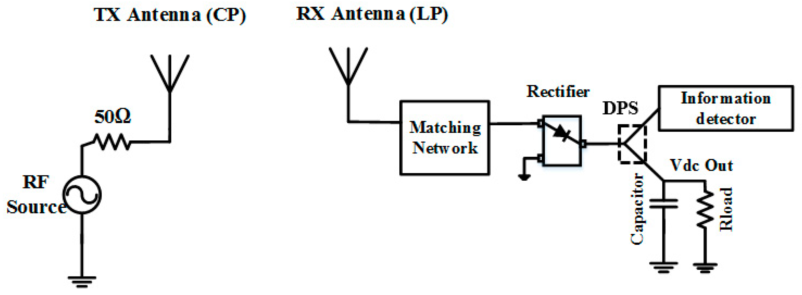
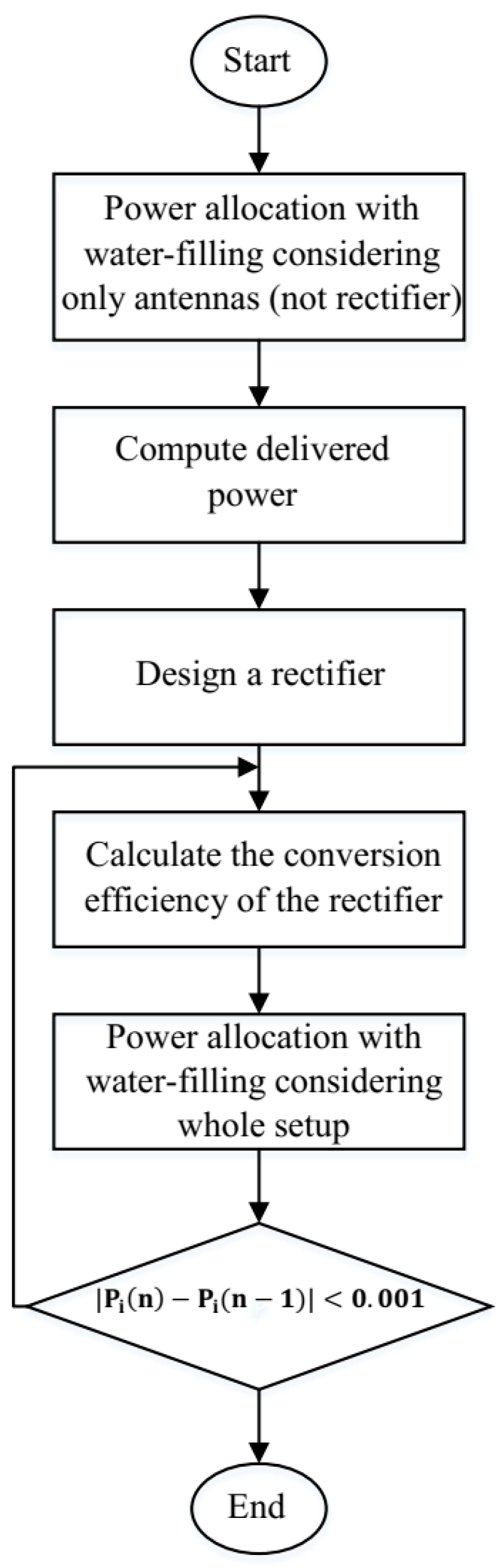
3. SWIPT System Design

One of the important parameters is the channel capacity in communication systems. The channel capacity represents the maximum achievable data rate for a communication channel. We use the unconstrained Shannon capacity formula for the AWGN channel [19]. It should be noted that this is an overestimation not only due to ignoring the modulation effect, but also due to ignoring the rectifier effect on noise. Since the rectifier is a nonlinear component, the whiteness assumption for noise is not fulfilled [20]. Notwithstanding, for the sake of simplicity, we use this well-known metric as an unreachable upper bound. The Shannon channel capacity for AWGN channel C s is a function of signal-to-noise ratio. It can be calculated per bandwidth segment, as follows [21]:
C s Δ B = log 2 ( 1 + P r P N ) ,
where Δ B is the bandwidth, P r is the received power, and P N is the noise power, which is assumed to be constant over the bandwidth. For M channels with equal bandwidth, the total channel capacity is as follows [21]:
C s = Δ B × m = 1 M log 2 ( 1 + P r ( f m ) P N )
where
P r ( f m ) = η p ( f m ) P i ( f m ) ,
where η p ( f m ) and P i ( f m ) are the ratio of delivered power to transmitted power ( P r P t ) and input power at the mth channel, respectively.
Based on Equation (3), higher bandwidths lead to a higher channel capacity. However, the power delivery trend is opposite, as the power transfer efficiency for single-stage rectennas has maximum at only one frequency. In order to increase the power delivery and channel capacity simultaneously, it is necessary to optimize power allocation, so the water-filling algorithm is used in this paper. Based on Lagrange optimization, the allotted power to maximize the Shannon channel capacity for the mth channel is as follows [15]:
P i ( f m ) = ( 1.44 λ P N η p ( f m ) )
where λ is the wavelength. Notice that only positive values of P i ( f m ) are acceptable. Negative values are converted to zero power. This formula is obtained with this assumption that the summation of the allotted power is equal to total transmitted power:
m = 1 M P i ( f m ) = P a v ,
At the receiver, the total amount of received power is defined, as follows:
P r = m = 1 M P r ( f m ) = m = 1 M P i ( f m ) η p ( f m ) ,
When the SWIPT receiver is a rectenna, it is essential to consider the efficiency of the rectifier in the water-filling algorithm. The conversion efficiency of the rectifier depends on both the frequency and input power. To consider this dependency in the water-filling algorithm, the flowchart of Figure 2 is proposed.
According to Figure 2, at the first step, it is assumed that the system does not include the rectifier and it consists of only two antennas. The allotted power to each channel using water-filling algorithm is calculated based on gain of the transmitter antenna, free space path loss, and gain of the receiver antenna. At the second step, a rectifier is designed regarding to the received power at the center frequency of bandwidth. Then, the efficiency of the rectifier is calculated for all the channels (according to output DC voltage and received power of each channel). Next, the ratio of delivered power (output DC power) to transmitted power while considering the conversion efficiency of the rectifier is calculated by Equation (1), then the water-filling algorithm is used to allot transmission power of each channel. Putting the rectifier design in the loop increases design complexity and risk of divergence. Therefore, it is constant during the power allocation. Iterations continue until the criterion P i ( n ) P i ( n 1 ) < 0.001   W is met where n and i refer to the iteration and the channel number, respectively. This condition means that the difference of two consecutive power transfers by the water-filling algorithm is too low, which does not affect the power delivery.
In the following, first, the narrowband set up is presented to demonstrate the algorithm, then the wideband set up is explained. It is assumed that the noise power P n = 10 8   W is fixed over the frequency where the power density in 300 MHz bandwidth is 135   dBm / Hz . This value is smaller comparison with the results in [16], this value is chosen. The total transmitted power is considered as P a v = 1   W .

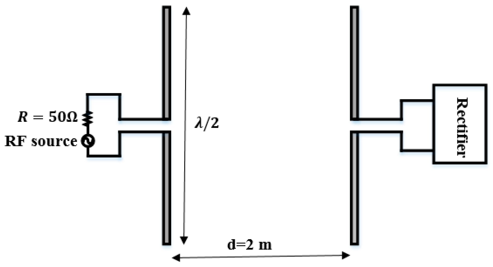
3.1. A SWIPT System Using Two Dipoles and a Narrow Band Rectifier

For the first step, two dipole antennas and a rectifier are assumed for a SWIPT system (Figure 3). As shown in Figure 3, two half wavelength dipoles at 1.44 GHz are separated by 2 m, where the length of each dipole is 9.15 cm. The impedance of source is 50 Ω and the bandwidth of the proposed setup is 300 MHz with 16 channels by the center frequency of 1.44 GHz. The simulated S 11 and the antenna realized gain are illustrated in Figure 4.
According to Friis’ transmission equation, the ratio of delivered power to transmitted power for two antennas separated by R meter can be calculated as follows:
P r P t = G t ( θ t , ϕ t ) G r ( θ t , ϕ t ) ( λ 4 π R ) 2 ( 1 | Γ t | ) 2 ( 1 | Γ r | ) 2 | a t . a r * | 2 e α R ,
where G t is the gain of transmitter antenna, G r is the gain of receiver antenna, Γ t is the reflection coefficient of transmitter, Γ r is the reflection coefficient of receiver, a t   and   a r are the polarization vectors of antennas, * is Hermitian transpose operator, and α is the absorption coefficient of the medium ( α = 0 for free space).
Based on Equation (8), the ratio ( P r P t ) of the two parallel dipole antennas with two meters distance is shown in Figure 5.
Now, we can calculate power of each channel based on proposed flow chart. After calculating the power of channels, the delivered power of RX for each channel is computed by Equation (8). The delivered power to RX antenna is the input power of the rectifier. Then, a rectifier is designed at the input power of center frequency (1.44 GHz), because the P r P t is maximum at the center frequency. For the sake of integrity, the design of rectifier is explained in the next section.
After calculating the conversion efficiency of the rectifier for each channel again, the transmission power is calculated by the water-filling algorithm and the condition is checked. If it is not satisfied, then the conversion efficiency of the rectifier is recalculated (based on new delivered power). This procedure continues iteratively until the condition is satisfied. For this configuration, after seven iterations, the condition is satisfied. The input power of the rectifier and the conversion efficiency of the rectifier for the first iteration are illustrated in Figure 6.
As shown in Figure 6, the highest efficiency occurs at 1.44 GHz where the input power is 22.8 dBm and the efficiency is 33%.
The channel capacity versus power delivery based on Equation (3) is shown in Figure 7. This Pareto front is plotted for 16 channels with 20 MHz bandwidth. As shown in Figure 7, when the set up includes just two dipole antennas, for one channel (center frequency) the channel capacity is 0.3 Gbit/s and the power delivery is 85   μ W . Also, for 16 channels, the power delivery is 63 μ W and the Shannon channel capacity is 2.74 Gbit/s. Therefore, when the number of channels increases, the power delivery decreases and the channel capacity jumps to the highest point.
After adding the designed rectifier, in the first iteration, the values P i for three channels are negative and these channels are deleted. It means that the setup with the assumption of 16 channels and P a v = 1   W cannot be realized and the number of channels should be decreased in order to allocate the transmitted power. So, for 13 channels, the power delivery is 7.2 μ W and the channel capacity is 1.05 Gbit/s. By increasing the number of iterations, after seven iterations, three more channels are also deleted and for the remaining 10 channels, the power delivery is increased to 10.8 μ W and the Shannon channel capacity reaches 1.15 Gbit/s, so both power delivery and the Shannon channel capacity are increased when compared to the first iteration. Therefore, the proposed algorithm not only considers the rectifier conversion efficiency, but also optimizes the SWIPT system and increases both channel capacity and power delivery.
In order to compare presented power allocation method (iterative water-filling algorithm) with the equal power allocation, the Pareto fronts of Shannon capacity versus power delivery are drawn in Figure 7. As shown in Figure 7, when the set up contains two dipole antennas, for the first 10 channels in which S 11 < 10   dB , there is no difference between water-filling algorithm and the equal power allocation. It is obvious that when the number of channels increases, the water-filling algorithm has a better result, because in the water-filling algorithm, the allotted power is determined with the respect of P r P t , but the equal power allocation does not consider P r P t . The difference of power delivery and channel capacity for water-filling algorithm compared with the equal power allocation are 10.5   μ W and 0.9   Gbit / s , respectively. As illustrated in Figure 7, the power delivery of equal power scenario is less than the water-filling set up.
As observed, using a narrowband subsystem reduces the number of channels and therefore capacity. Using wideband subsystems allows to use more channels efficiently, which will be shown in Section 5 (Figure 26).

4. Component Design

As it is mentioned in Section 2, the proposed set up in this article includes a broadband CP antenna as a transmitter, a broadband LP antenna, and a rectifier as a receiver. Designing the rectifier, the transmitter antenna and the receiver antenna are expressed in the following.

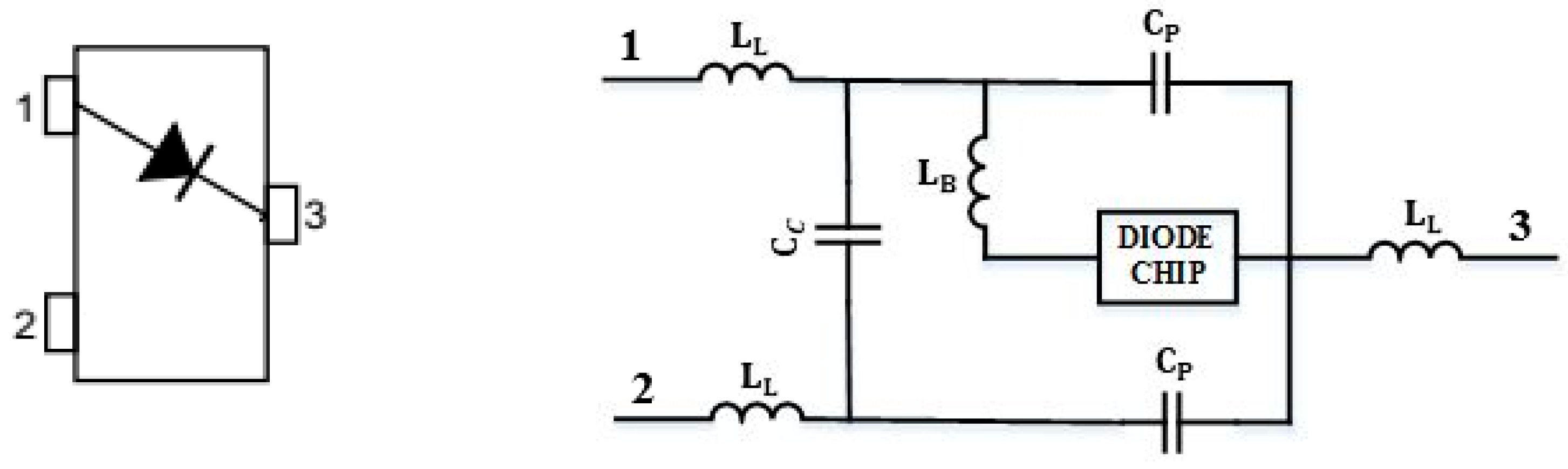
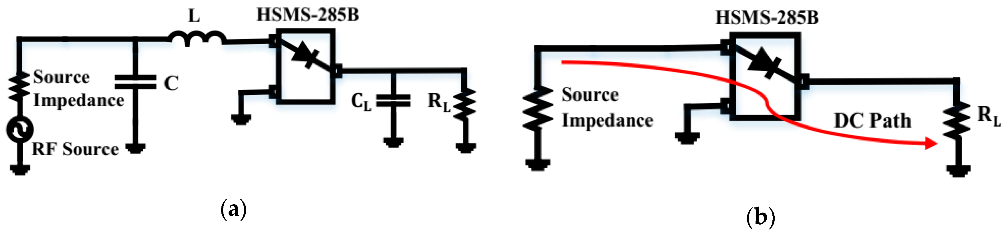
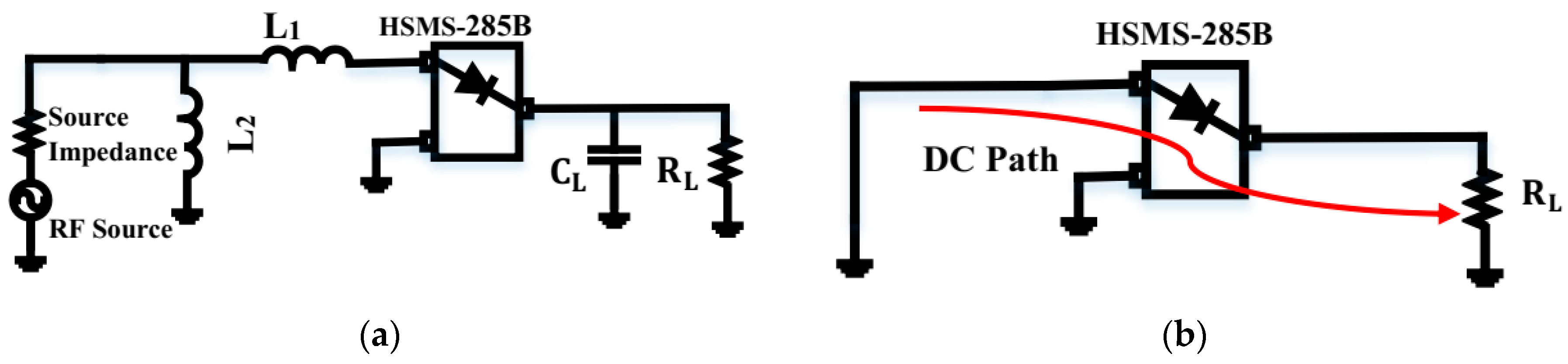
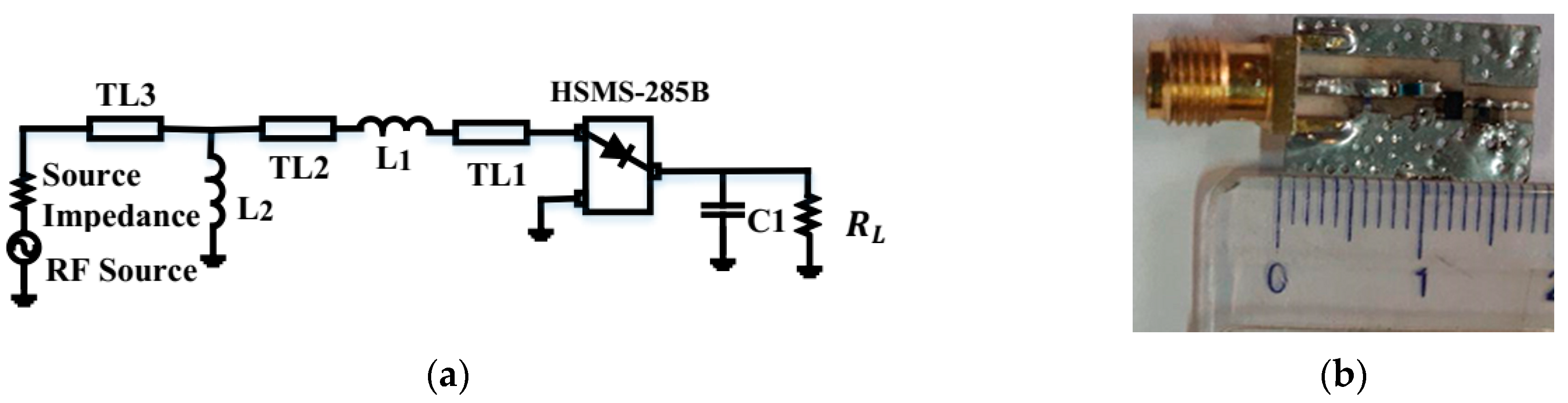
4.1. Rectifier Circuit

Rectifying circuits work on the base of nonlinear properties of semiconductor devices (diodes). These circuits convert unmodulated RF input signal to DC voltage. Their operations in time and frequency domain are shown in Figure 8.
A representative parameter showing the rectifier performance is conversion efficiency. In this study, a zero bias schottky diode, HSMS-285B in SOT 323 package [22], is used. In order to simulate the circuit, the equivalent linear models for diode [23] is used. It should be noted that the library model of conventional CAD software (ADS) is not accurate for design. Not only that models consider a parallel capacitance in each terminal to ground, but also the value of the presented elements in [23], which is used in ADS, are different. The SOT-323 package is illustrated in Figure 9. The L L is the leadfarm inductance, C P is the package capacitance, C c is the coupling capacitance between pin 1 and 2, and L B is bondwire inductance. The Spice parameters of diode chip are Rs = 25 Ω, Cj0 = 0.18 pF, EG = 0.69 V, and VB = 3.8 V [22]. The measured input impedance of the diode versus frequency when the input power is −30 dBm and the load resistance is 1   M Ω has been reported in [24]. The value of package parameters obtained in [24] is illustrated in Table 1.
According to [22], when the input power is higher than −20 dBm, diodes work in the large-signal regime, so the input impedance not only depends on frequency but also depends on input power [25]. It is also worth noting that surface mount assembly profile during assembly process must be applied [22] to function the diode properly and track the simulation results.
As mentioned in Section 3.1, the center frequency is 1.44 GHz and the input power of the rectifier is −22.8 dBm in this frequency. The load resistance in this work has been obtained through simulation with various load resistances and comparing with [26]. The input impedance of the rectifier is 6.9 169   j when the load resistance is 20 K Ω and C L = 100   pF , so the matching network should include a series inductance and a parallel capacitance.
It should be noted that designing a matching network is so important to properly operate the circuit, because the rectifier works in two modes. One mode is the fundamental frequency mode and the other one is the DC mode. In DC mode, the DC current path should be closed. If it is simulated in CAD, like Figure 10a, the current DC path would be like Figure 10b, but this circuit does not work in reality because our source is an antenna and it is not like a 50 ohm series resistance in DC mode. Therefore, the matching should be changed and it includes a series and a parallel inductance (Figure 11a), which the DC path is illustrated in Figure 11b. In consequence, the modified design for rectifier is illustrated in Figure 11b.
The elements of matching network are as follows: L1 is 32 nH and L2 is 2.2 nH.

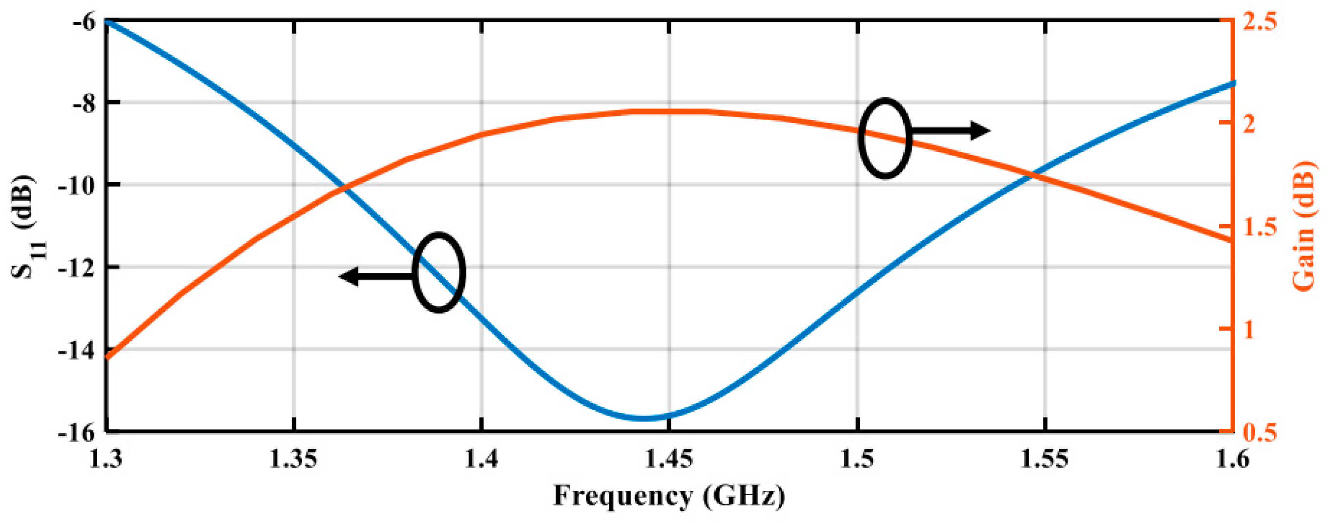
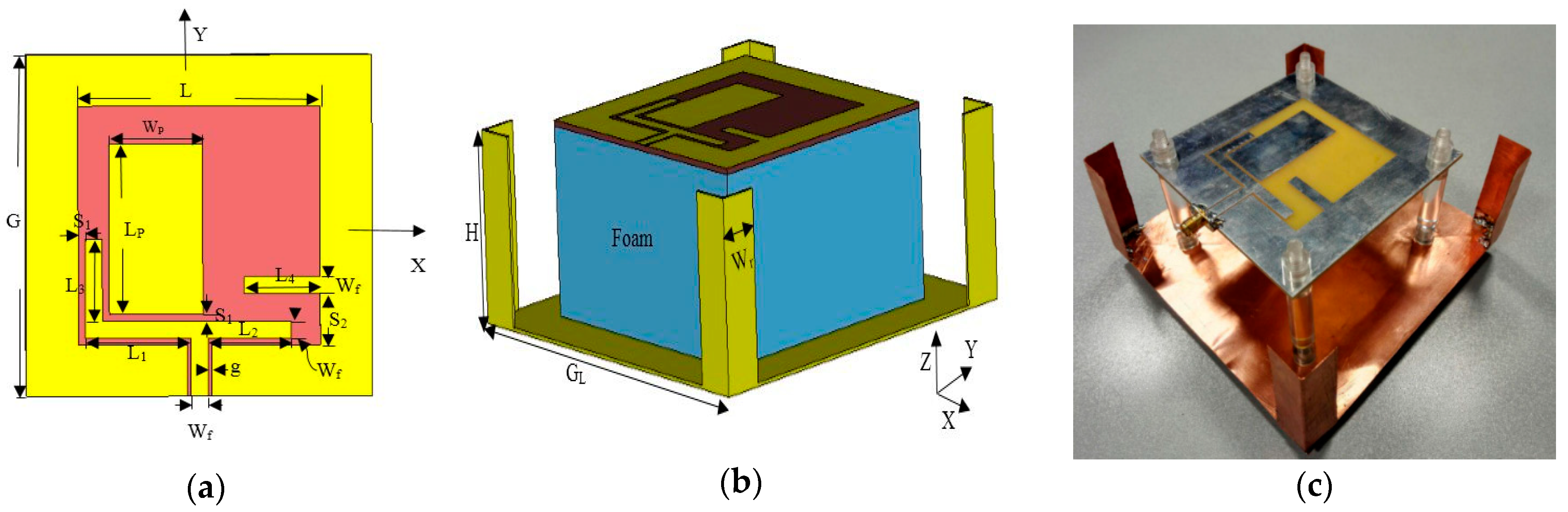
4.2. Transmitter (TX) Antenna

As mentioned in the introduction, using CP antenna in one side of link, mitigates the fading resulted from random alignment of target. Since the wideband CP antenna in this frequency needs a more complicated structure, we put it at the transmitter, and used simpler LP antenna at the receiver. The challenge of designing TX antenna is a broadband axial ratio. In order to have a broadband CP antenna, square slot antennas with coplanar waveguide (CPW) fed is recommended [27,28,29]. Not only do these structures enhance the axial ratio bandwidth, but also the impedance bandwidth would be increased. Based on [27], a broadband CP slot antenna is designed and illustrated in Figure 12. It is fabricated on FR-4 substrates with ε r = 4.3 , tan δ = 0.02 , and thickness (h) of 1.6 mm.
As shown in Figure 12a, the antenna is fed with a CPW line. w f and g provide 50 ohm CPW transmission line. The CPW line is connected to L-shaped metal. The length of this L-shaped metal and the asymmetric shape of it are consequential to obtain CP operation. The rectangular metal patch with the dimension of L P × W P extends axial-ratio bandwidth. In addition, the stub with the length of L 4 and width of W f with the height of S 2 from lower edge is added to enhance impedance bandwidth and reduce the size. In order to increase the gain of the antenna, a square metal reflector with the length of G L is located at λ 0 / 4 below the patch, where λ 0 is the free-space wavelength at the center frequency, so the reflected backward waves from the reflector have the same phase and polarization with the forward radiated waves [27]. All of the required dimensions of the antenna with reflector are presented in Table 2.
Figure 13 and Figure 14 show the simulated and measured S 11 and the axial ratio of the TX antennas versus frequency, respectively.
As shown in Figure 13, the impedance bandwidth of the antenna is 45% in the center frequency of 1.44 GHz (1.1–1.75 GHz). As illustrated in Figure 14, the axial-ratio bandwidth is 25% in the center frequency of 1.44 GHz (1.25–1.6 GHz). This makes it suitable for using as transmitter in the SWIPT system.
The simulated and measured radiation pattern in two different planes (phi = 0 and phi = 90) at 1.44 GHz are shown in Figure 15.
As shown in Figure 15a,b, using the reflector has resulted in 10 dB front to back ratio.

4.3. Receiver (RX) Antenna

As mentioned in Section 2, the receiver antenna should be broadband and has linearly polarized radiation. Generally, there are some methods to increase impedance bandwidth, such as U-shaped slot, stacked structures, cutting the ground of the structure, like ultra wide band (UWB) antennas, and etc. [30]. The first two methods cannot support the recommended bandwidth (1.3–1.6 GHz), so the method that provides this bandwidth is an UWB antenna. Therefore, a broadband linearly polarized patch antenna is designed based on [31]. Figure 16 shows the configuration of the antenna. It is fabricated on FR-4 substrates with ε r = 4.4 , tan δ = 0.02 , and thickness (h) of 1.6 mm.
The antenna is a printed CPW-fed half elliptical monopole. CPW-fed is 50 ohm. According to simulation, the surface current of the patch on the bottom apex and along the margin of the patch is maximum and in center of patch is zero. It means that the center of the half elliptical patch does not affect the radiation (it is shown in Figure 17), so we can cut half of the metal of the patch and reduce the metal surface without impacting on the antenna performance. The antenna dimensions are presented in Table 3. As a rule of thumb in printed UWB monopole antenna design, at the lowest resonance frequency, R1 must be around λ 0 4 , which mimics a quarter wavelength monopole antenna [32]. However, again similar to monopole antennas, width of radiating part (R3) also affects the resonant frequency. The final antenna dimensions are listed in Table 3.
The simulated and measured reflection coefficient of RX antenna is plotted in Figure 18. As can be seen, there is an upper shift in measurement, which is probably due to uncertainty of the applied FR4 dielectric constant. However, the impedance bandwidth of the antenna is still 720 MHz and covers our system requirements that are described in Section 2.
The simulated and measured radiation pattern in two different planes (phi = 0 and phi = 90) at 1.44 GHz are illustrated in Figure 19.
The discrepancy between measurement and simulation might be due to uncertainty of our anechoic chamber, which is not perfect below 2 GHz. However, since the TX antenna radiates CP, and the link was designed with the assumption of a movable RX, the RX pattern rotation is not very important in practice. In the next section, the result of involving these component in the final system will be presented.

5. Proposed Broadband SWIPT Setup

In this section, the broadband SWIPT system and its performance are analyzed. For this purpose, three different scenarios are considered. First, two broadband antennas are considered, then it is assumed that the receiver contains a narrowband rectenna (the broadband LP antenna and a narrowband rectifier), and finally, the broadband rectenna is considered as a receiver. The channel capacity versus the power delivery of these configurations are compared and discussed.

5.1. A SWIPT System Using Two Broadband Antennas

As mentioned, the transmitter is a broadband CP antenna and the receiver is a broadband linearly polarized antenna. The broadside realized gain of the TX and RX antennas versus frequency are shown in Figure 20.
The ratio of ( P r P t ) for two supposed antennas with 2 m distance based on Equation (9) is illustrated in Figure 21.
As shown in Figure 21, the ratio of ( P r / P t ) is decreased by increasing the frequency due to free space loss. According to the ratio of ( P r / P t ) , the Pareto front of the channel capacity versus power delivery will be illustrated in Figure 26. However, for wireless power transmission realization, a rectifier is necessary. Introducing the rectifier in the link degrades the performance; but the proper design of it can alleviate this degradation. Two cases of narrowband and wideband rectifiers will be compared in the next subsections.

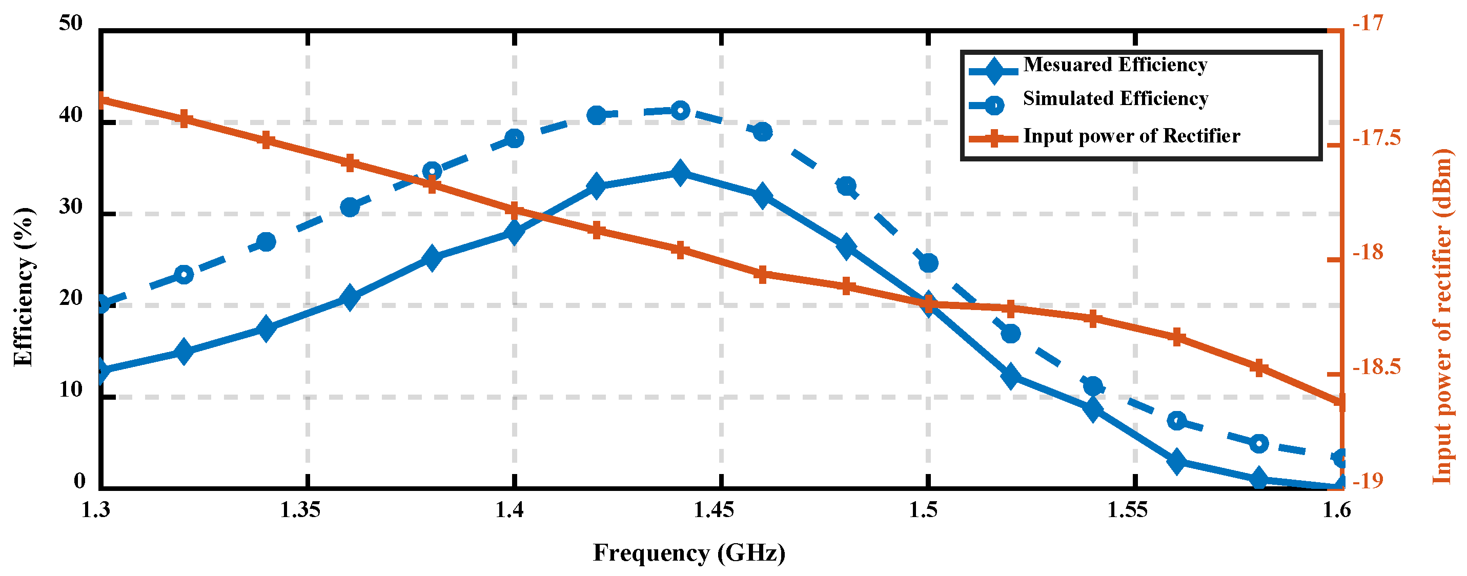
5.2. A SWIPT System Using Two Broadband Antennas and a Narrowband Rectifier

The ratio of ( P r / P t ) for two broadband antennas was calculated in pervious section, and in this part, it is assumed that the receiver also has a rectifier. Based on the proposed flow chart in Figure 2, after calculating the allotted power according to the water-filling algorithm with assumption P a v = 1   W and P N = 10 8   W , at the second step, the input power of the rectifier from Equation (4) is calculated. In the center frequency (1.44 GHz), the input power of the rectifier is −17.59 dBm. A narrowband rectifier, like Section 4.1 at 1.44 GHz with the input power −17.59 dBm, is designed. With this input power, the input impedance of the rectifier at 1.44 GHz is 5.09 j 169.87   Ω . The configuration of the simulated and implemented rectifier is shown in Figure 22. It was fabricated on RO4003 with ε r = 3.38 . The load resistance is 20K Ω , C1 is 100 PF and the matching network consist of a series inductance (L1 = 18 nH) and a parallel inductance (L2 = 2.2 nH). The TL1 and TL2 microstrip lines are used to mount the pins of diode and smd inductor, respectively. TL3 microstrip line is 50 ohm and it is added to mount the SMA (Sub Miniature version A) connector.
After designing the rectifier, its conversion efficiency is considered in the power allocation algorithm (water-filling) and the allotted power is calculated for each channel. Again, the conversion efficiency of the rectifier based on new input power is calculated, and it continuous until the stop condition is satisfied (here after two iterations). At the end, the results of simulation and measurement of the conversion efficiency of rectifiers after two steps of the iteration algorithm for 16 channels with different input power are illustrated in Figure 23. It is observed that, when the antennas are broadband, the number of iterations decrease and the algorithm converges rapidly.
The simulated conversion efficiency of the rectifier is 41% when the input power is −17.95 dBm at 1.44 GHz, and this value is acceptable when compared with [26,33]. The measured efficiency at this frequency and input power is 34.5% and the DC output voltage is 0.331 V. The corresponding diagram of the channel capacity versus power delivery will be plotted in Figure 26.

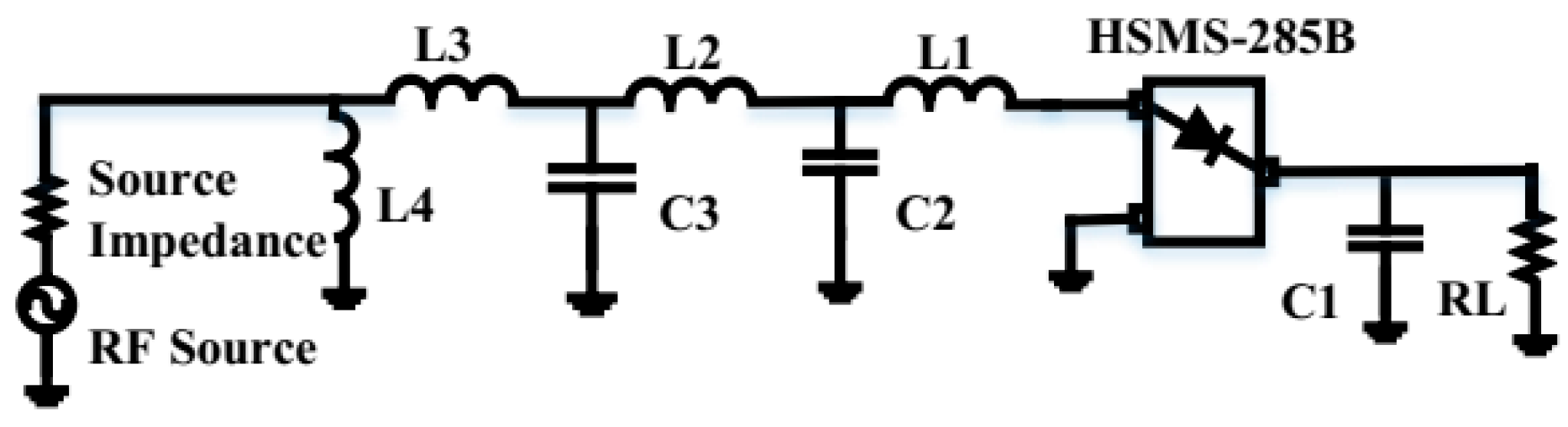
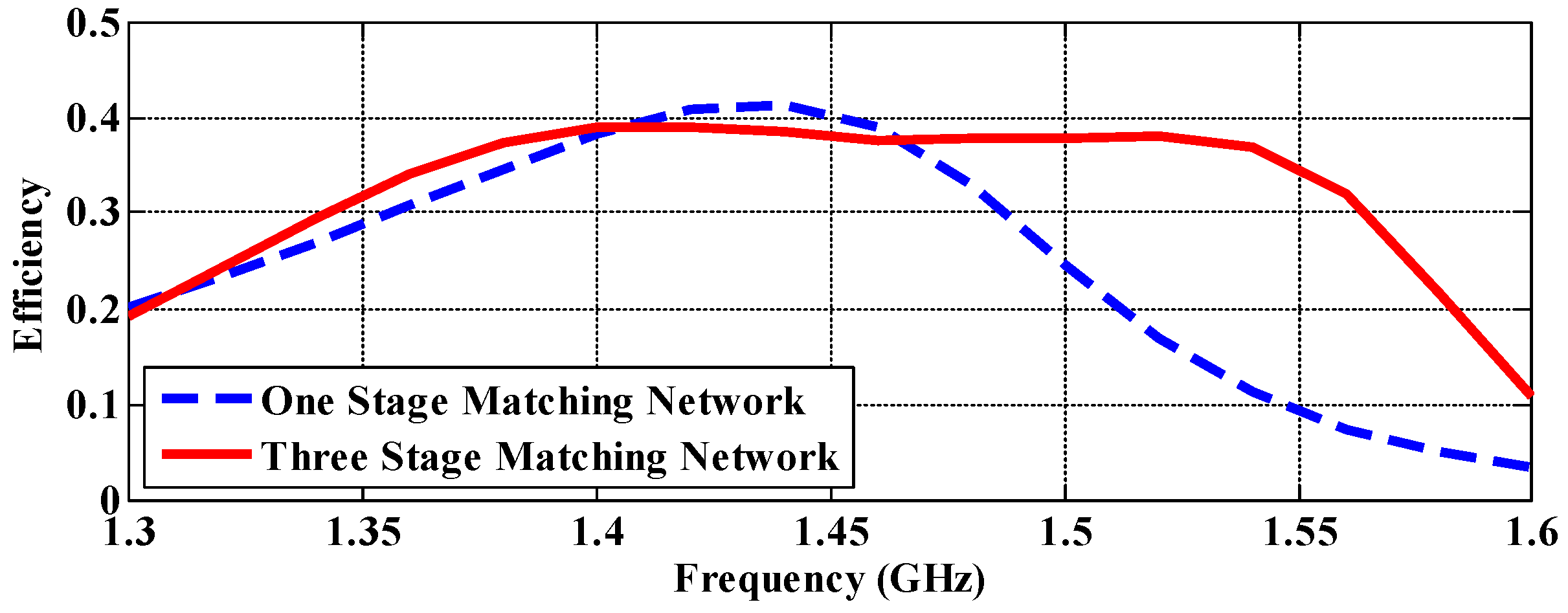
5.3. A SWIPT System Using Two Broadband Antennas and a Broadband Rectifier

In previous section, the matching network of rectifier was narrowband. In order to increase the bandwidth of the matching network, two stages are added to the matching network. The target is flatting the conversion efficiency over the frequency in different input powers. The configuration of designed matching network is shown in Figure 24. Using the ADS software optimization tool, the values listed in Table 4 were obtained.
The conversion efficiency diagram of the broad band rectifier in comparison to the narrowband rectifier is shown in Figure 25. As can be seen, the conversion efficiency of narrowband rectifier is higher than 30 percent for six channels. However, the conversion efficiency of broadband rectifier is higher than 30 percent for 13 channels.
The Pareto front of the channel capacity versus power delivery based on the proposed power allocation algorithm for three different cases (two broadband antennas without considering rectifier, broadband antennas and narrowband rectifier, and broadband antennas with broadband rectifier) is shown in Figure 26.
As shown in Figure 26, when the set up contains two broadband antennas (which means inefficiency of rectifier has been ignored), the power delivery is 260 μ W and the channel capacity is 3.45 Gbit/s for 16 channels. Adding narrowband rectifier to system model reduced power delivery and channel capacity to 35 μ W and 2.16 Gbit/s, respectively. When the rectifier is broadband, the maximum conversion efficiency decreases, but it is more than 30% for more channels when compared with the narrowband rectifier. This causes the broadband rectifier to have less power delivery for one channel, but when the number of channels increases it overpasses the narrowband rectifier i.e., the channel capacity and the power delivery for broadband rectifier increase in compression with the narrowband one. For broadband setup, the power delivery is 79 μ W and the channel capacity is 2.86 Gbit/s for 16 channels. It is obvious that the channel capacity and the power delivery of broadband system is increased to 0.7 Gbit/s and 44 μ W , respectively, when compared to narrowband rectifier. Therefore, as can be seen from Figure 26, to properly design a SWIPT system, the rectifier should be considered.
Similar to Section 3.1, to compare the equal power allocation with presented allocation power in this article, the channel capacity versus power delivery for three different types are drawn in Figure 26. It is illustrated that when the set up includes wideband antennas, the power allocation method does not influence on power delivery and channel capacity. However, if the set up contains WB antennas and a narrowband rectifier, the performance of power allocation appears for higher channels. For 16 channels, the power delivery and channel capacity that were obtained by water-filling algorithm are 3   μ W and 0.03   Gbit / s higher than the equal power allocation. Finally, for wideband antennas and wideband rectifier these differences are too low ( 0.03   μ W and less than 0.001   Gbit / s ), which can be neglected.

6. Conclusions

In this paper, a broadband SWIPT system was implemented and analyzed. To consider the random change of antenna directions, the transmitter was broadband CP antenna and the receiver includes broadband LP antenna and rectifier. In addition, an iterative algorithm for SWIPT systems when the receiver includes rectenna was proposed. To explain the concept, three different SWIPT scenarios consist of two broadband antennas, two broadband antennas with narrowband rectifier, and finally, two broadband antennas with broadband rectifier are considered. The results show that ignoring the rectifier in the model overestimates channel capacity and power delivery capabilities. Considering the rectifier provides weaker but more reliable Pareto fronts. According to the Pareto fronts, including rectifier, when the rectifier is broadband, the Shannon channel capacity and power delivery increases 0.7 Gbit/s and 44 μ W , respectively, as compared to narrowband one.

Author Contributions

Investigation, M.S., and A.A.; Supervision, S.C.; Project administration, A.A.; Validation, G.D.G., Original draft preparation, M.S., and A.A.; Review and editing of the final manuscript, S.C., and G.D.G.

Funding

This research received no external funding.

Conflicts of Interest

The authors declare no conflict of interest.

References

  1. Perera, T.D.P.; Jayakody, D.N.K.; Sharma, S.K.; Chatzinotas, S.; Li, J. Simultaneous Wireless Information and Power Transfer (SWIPT): Recent Advances and Future Challenges. IEEE Commun. Surv. Tutor. 2017, 20, 264–302. [Google Scholar] [CrossRef]
  2. Xu, Y.; Ding, Z.; Sun, X.; Yan, S.; Zhu, G.; Zhong, Z. Joint Beamforming and Power-Splitting Control in Downlink Cooperative SWIPT NOMA Systems. IEEE Trans. Signal Process. 2017, 65, 4874–4886. [Google Scholar] [CrossRef] [Green Version]
  3. Boshkovska, E.; Kwan Ng, D.W.; Zlatanov, N.; Schober, R. Practical Non-Linear Energy Harvesting Model and Resource Allocation for SWIPT systems. IEEE Commun. Lett. 2015, 19, 2082–2085. [Google Scholar] [CrossRef]
  4. Yao, Y.; Wu, J.; Shi, Y.; Dai, F.F. A fully integrated 900-MHz passive RFID transponder front end with novel zero-threshold RF-DC rectifier. IEEE Trans. Ind. Electron. 2009, 56, 2317–2325. [Google Scholar] [CrossRef]
  5. Kim, Y.; Lee, T.J.; Kim, D.I. Joint Information and Power Transfer in SWIPT-enabled CRFID Networks. IEEE Wirel. Commun. Lett. 2017, 2337, 186–189. [Google Scholar] [CrossRef]
  6. Popovic, Z.; Falkenstein, E.A.; Costinett, D.; Zane, R. Low-power far-field wireless powering for wireless sensors. Proc. IEEE 2013, 101, 1397–1409. [Google Scholar] [CrossRef]
  7. Nishimoto, H.; Kawahara, Y.; Asami, T. Prototype implementation of ambient RF energy harvesting wireless sensor networks: A review. Renew. Sustain. Energy Rev. 2015, 45, 769–784. [Google Scholar] [CrossRef]
  8. Akyildiz, I.F.; Melodia, T.; Chowdhury, K.R. A survey on wireless multimedia sensor networks. Comput. Netw. 2007, 51, 921–960. [Google Scholar] [CrossRef] [Green Version]
  9. Kim, S.; Vyas, R.; Bito, J.; Niotaki, K.; Collado, A.; Gerogiadis, A.; Tentzris, M.M. Ambient RF energy-harvesting technologies for self-sustainable standalone wireless sensor platforms. Proc. IEEE 2014, 102, 1649–1666. [Google Scholar] [CrossRef]
  10. Chen, H.H.; Li, Y.; Jiang, Y.; Ma, Y.; Vucetic, B. Distributed Power Spilitting for SWIPT in Relay Interference Channels Using Game Theory. IEEE Trans. Wirel. Commun. 2015, 14, 410–420. [Google Scholar] [CrossRef]
  11. Zhang, J.; Yuen, C.; Wen, C.K.; Jin, S.; Wong, K.K.; Zhu, H. Large system secrecy rate analysis for SWIPT MIMO wiretap channels. IEEE Trans. Inf. Forensics Secur. 2016, 11, 74–85. [Google Scholar] [CrossRef]
  12. Zhang, R.; Ho, C.K. MIMO broadcasting for simultaneous wireless information and power transfer. IEEE Trans. Wirel. Commun. 2013, 12, 1989–2001. [Google Scholar] [CrossRef]
  13. Krikidis, I.; Sasaki, S.; Timotheou, S.; Ding, Z. A low complexity antenna switching for joint wireless information and energy transfer in MIMO relay channels. IEEE Trans. Commun. 2014, 62, 1577–1587. [Google Scholar] [CrossRef]
  14. Zhou, X.; Zhang, R.; Ho, C.K. Wireless Information and Power Transfer: Architecture Design and Rate-Energy Tradeoff. IEEE Trans. Commun. 2013, 61, 4754–4767. [Google Scholar] [CrossRef]
  15. Caspers, E.P.; Yeung, S.H.; Sarkar, T.K.; Lamperez, A.G. Analysis of Information and Power Transfer in Wireless Communications. IEEE Antenna Propag. Mag. 2013, 55, 82–95. [Google Scholar] [CrossRef]
  16. Yeung, S.H.; Sarkar, T.K.; Salazar-Palma, M.; Lagunas, M.A.; Perez-Neira, A.I. Broadband Matching in Simultaneous Information and Power Transfer. IEEE Antenna Propag. Mag. 2015, 57, 192–203. [Google Scholar] [CrossRef]
  17. Krikidis, I.; Timotheou, S.; Nikolaou, S.; Zheng, G.; Ng, D.W.K.; Schober, R. Simultaneous Wireless Information and Power Transfer in modern communication systems. IEEE Commun. Mag. 2014, 52, 104–110. [Google Scholar] [CrossRef]
  18. Liu, L.; Zhang, R.; Chua, K.C. Wireless Information and Power Transfer: A Dynamic Power Splitting Approach. IEEE Trans. Commun. 2013, 61, 3990–4001. [Google Scholar] [CrossRef] [Green Version]
  19. Forney, G.D.; Ungerboeck, G. Modulation and Coding for Linear Gaussian Channels. IEEE Trans. Inf. Theory 1998, 44, 1807–1813. [Google Scholar] [CrossRef]
  20. Wolf, M.; Cheema, S.A.; Haardt, M. PAM-transmission with optimal detection for dispersive optical channels with intensity modulation and direct detection. In Proceedings of the Transparent Optical Networks (ICTON), Girona, Spain, 2–6 July 2017. [Google Scholar] [CrossRef]
  21. Shannon, C.E. Communication in the Presence of Noise. Proc. IEEE 1998, 68, 447–457. [Google Scholar] [CrossRef]
  22. HSMS-285x Surface Mount RF Schottky Barrier Diodes, Data Sheet; Avago Technologies: San Jose, CA, USA, 2004.
  23. Linear Models for Diode Surface Mount Packages, Application Note 1124; Hewlett Packard: Palo Alto, CA, USA, 1997.
  24. Nimo, A.; Grgić, D.; Reindl, L.M. Optimization of Passive Low Power Wireless Electromagnetic Energy Harvesters. Sensors 2012, 12, 13636–13663. [Google Scholar] [CrossRef] [PubMed] [Green Version]
  25. Maas, S.A. Nonlinear Microwave and RF Circuits, 2nd ed.; Artech House: Londan, UK, 2003; pp. 115–211. ISBN 978–1580534840. [Google Scholar]
  26. Visser, H.J.; Keyrouz, S.; Smolders, A.B. Optimized rectenna design. Wirel. Power Transf. 2012, 2, 44–50. [Google Scholar] [CrossRef]
  27. Sze, J.Y.; Chang, C.C. Circularly polarized square slot antenna with a pair of inverted-L grounded strips. IEEE Antennas Wirel. Propag. Lett. 2008, 7, 149–151. [Google Scholar] [CrossRef]
  28. Chen, Y.B.; Liu, X.F.; Jiao, Y.C.; Zhang, F.S.; Edition, S. CPW-fed broadband circularly polarised square slot antenna. Electron. Lett. 2006, 42, 1074–1075. [Google Scholar] [CrossRef]
  29. Pan, S.P.; Sze, J.Y.; Tu, P.J. Circularly polarized square slot antenna with a largely enhanced axial-ratio bandwidth. IEEE Antennas Wirel. Propag. Lett. 2012, 11, 969–972. [Google Scholar] [CrossRef]
  30. Allen, B.; Dohler, M.; Okan, E.E.; Malik, W.Q.; Brown, A.K.; Edwards, D.J.; Adatia, N. Theory of UWB Antenna Elements. In Ultra-Wideband Antennas and Propagation for Communication, Radar and Imaging; Wiley: London, UK, 2007; ISBN 978–0-470-03255-8. [Google Scholar]
  31. Ding, W.; Liu, S.; Zhan, B.; Wang, G. A miniaturized ultra-wideband CPW-fed antenna. In Proceedings of the 2015 IEEE MTT-S International Conference on Numerical Electromagnetic and Multiphysics Modeling and Optimization (NEMO), Ottawa, ON, Canada, 11–14 August 2015. [Google Scholar] [CrossRef]
  32. Fereidoony, F.; Chamaani, S.; Mirtaheri, S.A. Systematic Design of UWB Monopole Antennas with Stable Omnidirectional Radiation Pattern. IEEE Antenna Wirel. Propag. Lett. 2015, 11, 725–755. [Google Scholar] [CrossRef]
  33. De Donno, D.; Catarinucci, L.; Tarricone, L. An UHF RFID energy-harvesting system enhanced by a DC-DC charge pump in silicon-on-insulator technology. IEEE Microw. Wirel. Compon. Lett. 2013, 23, 315–317. [Google Scholar] [CrossRef]
Figure 1. Proposed set up.
Energies 11 02387 g001
Figure 2. Iterative algorithm flow chart includes water-filling algorithm.
Energies 11 02387 g002
Figure 3. Configuration of two dipoles.
Energies 11 02387 g003
Figure 4. Simulated S 11 and gain for dipole antenna.
Energies 11 02387 g004
Figure 5. P r / P t of two dipole antennas.
Energies 11 02387 g005
Figure 6. Input power and conversion efficiency of rectifier for first iteration.
Energies 11 02387 g006
Figure 7. Pareto fronts of Shannon capacity versus power delivery in different cases.
Energies 11 02387 g007
Figure 8. The operations of rectifiers in time and frequency domain.
Energies 11 02387 g008
Figure 9. Linear model of HSMS-285B [23].
Energies 11 02387 g009
Figure 10. (a) First design for rectifier; (b) DC path for this design.
Energies 11 02387 g010
Figure 11. (a) Modified design for rectifier; (b) DC path of designed rectifier.
Energies 11 02387 g011
Figure 12. Configuration of presented circularly polarized (CP) square slot antenna; (a) slot patch antenna top view; (b) antenna with reflector; and, (c) implemented antenna.
Energies 11 02387 g012
Figure 13. Simulated and measured return loss of the TX Antenna.
Energies 11 02387 g013
Figure 14. Simulated and measured the axial-ratio of the TX Antenna.
Energies 11 02387 g014
Figure 15. Simulated (dashed line) and measured (solid line) radiation pattern (a) ϕ = 0 ° ; (b) ϕ = 90 ° .
Energies 11 02387 g015
Figure 16. (a) Top view of receiver (RX) antenna; (b) fabricated printed CPW-fed half elliptical monopole.
Energies 11 02387 g016
Figure 17. (a) The current density for complete antenna; (b) the current density for half elliptical antenna.
Energies 11 02387 g017
Figure 18. Measured and simulated S 11 of the RX antenna.
Energies 11 02387 g018
Figure 19. Simulated (dashed line) and measured (solid line) radiation pattern (a) ϕ = 0 ° ; (b) ϕ = 90 ° .
Energies 11 02387 g019
Figure 20. Realized gain of transmitted and received antenna versus frequency.
Energies 11 02387 g020
Figure 21. The ratio of P r / P t of broadband antennas without rectifier.
Energies 11 02387 g021
Figure 22. (a) Simulated rectifier; (b) implemented rectifier.
Energies 11 02387 g022
Figure 23. Measured and simulated efficiency of the rectifier and its input power.
Energies 11 02387 g023
Figure 24. The configuration of simulated broadband rectifier.
Energies 11 02387 g024
Figure 25. Simulated conversion efficiency of broadband rectifier (solid) and narrowband rectifier (dashed).
Energies 11 02387 g025
Figure 26. Pareto front of the Shannon capacity versus power delivery for different cases with different power allocation methods.
Energies 11 02387 g026
Table 1. Value of diode elements.
Element C C C P L L L B
Value 0.214   pF 0.184   pF 0.5   nH 0.7   nH
Table 2. Dimensions of the Tx antenna based on Figure 12 (unit: mm).
GLL1L2L3L4WfgWPLPS1S2GLHWr
1006026.520182250.523461151405015
Table 3. Dimensions of RX antenna (unit: mm).
LWWfgdR1R2R3R4
11511040.510101527025
Table 4. The values of matching network in Figure 24.
RLC1L1L2L3L4C2C3
20   K Ω 100 (pF)22 (nH)2.53 (nH)4.5 (nH)2.2 (nH)7.34 (pF)2.27 (pF)

