Simulation of a Fluidized Bed Dryer for the Drying of Sago Waste

Abstract

The large amount of sago waste produced by sago processing industries can cause serious environmental problems. When dried, these residues usually have a high starch content (around 58%) and have many potential applications. In this study, the drying of sago waste using a fluidized bed dryer (FBD), which offers more advantages than other drying methods, is analyzed via computational fluid dynamics (CFD) modeling. A two-dimensional (2D) FBD model is also developed and a mesh independency test is conducted immediately afterwards. A fine mesh is selected for the CFD model and a simulation is conducted using ANSYS Fluent 17.1 software (Ansys Inc., version 17.1, Canonsburg, PA, USA). The governing and discretized algebraic equations are solved by applying the phase-coupled semi-implicit method for pressure-linked equations. Both the Eulerian–Eulerian multiphase model approach and the turbulence model are applied in the simulation due to the turbulent flow in the dryer. A velocity of 1.30 m/s and temperature of 50 °C are selected as boundary conditions based on the optimum parameter values from previous experiments. The final moisture content that we aim to achieve is 10% or a moisture ratio of 0.25 in sago waste for the purpose of animal feed, so as to prevent bacterial growth and for packaging purposes based on common industrial practice. Both the drying rate and fluidization profile are examined at air velocities of 0.6, 1.0, 1.3, 1.8, and 2.2 m/s. Based on the results, the velocity range of 1.0 m/s to 2.2 m/s is deemed suitable for the fluidization and drying of sago waste with a particle size of 2000 μm for a drying simulation of 1 h. The drying rate is further examined at air temperatures of 50 °C, 60 °C, 70 °C, and 80 °C, whereas the fluidization profile is examined at particle sizes of 200, 500, 1000, and 2000 μm. The results reveal excellent fluidization at a particle size range of 500 μm to 2000 μm and a velocity of 1.3 m/s.

1. Introduction

Sago palm (Metroxylon spp.) is a tropical plant that can adapt well in wet growing conditions [1]. Malaysia, especially Sarawak, is the largest sago exporter in the world and currently has nine sago processing industries that operate actively and export around 25,000 to 40,000 tons of sago products to Peninsular Malaysia, Japan, Taiwan, Singapore, and other countries [2]. However, the extraction of starch and the large-scale production of sago also generate sago waste or pith residues. Sarawak, especially its towns Sibu and Mukah, produces a large amount (at least 50 to 110 tons) of sago waste every day from their sago processing industries. These residues comprise 58% starch, 23% cellulose, 9.2% hemicellulose, and 4% lignin [3] and have many potential functions, such as in the manufacturing of textile printing materials [4]. Several studies have investigated other usages of sago waste, including their adsorption of lead and copper [5] as well as their use in the production of bioethanol [6].

Sago waste is usually mixed with wastewater and either discharged into streams or deposited in factory compounds. Each tone of extracted sago starch produces and dumps approximately one tone of sago waste into the nearby rivers. Data from the Malaysian Department of Statistics reveal that the country produced approximately 52,000 tons of sago starch in 2011. Nearly the same amount of sago waste was dumped in nearby rivers [7], thereby causing serious environmental problems such as water pollution. The high demand for biological oxygen (approximately 5820 mg/L) and chemical oxygen (approximately 10,220 mg/L) [1] in wastewater affects the marine life and water quality via microbiological degradation and by consuming the dissolved oxygen in the water. Some factories in Malaysia have started to burn these residues after realizing the negative effects of discharging these wastes into nearby streams. However, the combustion of sago can contribute to air pollution and wastage, considering of the reuse potential of sago waste [4].

Before reusing these materials, the moisture content of sago waste must be reduced by drying. Drying is a well-known method that is used in many industries, such as in the food industry, in order to inhibit bacteria and microorganism growth [8,9]. It is important to maintain the product quality such as color, textural attributes, and retained total polyphenol content (TPC) [10]. Several conventional drying methods are currently being applied, including sun- and oven-drying [11]. However, these methods consume much energy and may expose the dried waste to a dirty and dusty environment [12].

The most famous practical method for drying solid particles is the use of a fluidized bed dryer (FBD), which offers several advantages over other dryers (i.e., spray and cabinet dryers), including the high mass and heat transfer between the gas and solid phases, good mixing of solids, lower capital costs, and ease of operation and maintenance [8,13].

Drying via computational fluid dynamics (CFD) simulation is more beneficial than conducting experiments, given the lack of information regarding the requirements for achieving an optimum operation condition in the drying process. Many factors and parameters can affect the operation conditions. Firstly, achieving an optimum drying condition during the initial stages of the experiment entails a high cost and a long drying time. Secondly, some apparatuses, such as FBD, are also necessary. Thirdly, some problems may hinder the accurate measurement of the parameters and ultimately affect the drying process.

CFD generates discrete solutions for real-world fluid flow problems and uses various software tools to predict fluid flow, heat and mass transfer, chemical reaction, and other related phenomena at a low cost. Some studies have dried solids by conducting a CFD simulation. Mortier et al. [14] analyzed the application of FBD in drying wet granules in pharmaceutical processes. Several models have also been proposed, such as models in CFD tools and the population balance model, to describe the distribution of particle properties. These studies reveal that CFD modeling can improve the scientific understanding and optimize the drying process to a certain extent.

Mortier et al. [15] applied CFD to examine the heat and mass transfer process in the drying of wheat grains in an FBD. They also applied the Eulerian–Eulerian two-fluid model coupled with kinetic theory in the simulation of gas–solid flow to predict the temperature distribution and moisture of solids at various drying times. Several parameters were considered, including inlet gas velocity, inlet gas temperature, particle size, and initial solid moisture. Their findings showed that the FBD is highly sensitive to particle size, inlet gas temperature, and initial solid moisture, while the air velocity can shorten the drying time.

P. Sahoo and A. Sahoo [16] examined the fluidization of coarse and fine particles in a fluidized bed by conducting a simulation in ANSYS Fluent 13.0. They employed the Gidaspow drag model in the simulation to compare with the experimental study for pressure drop variations and bed height changes. It was found that the simulation and experimental outcome showed a close approximation.

2. Methodology

Numerical simulation required the type of model, properties of parameters on each boundary, and the operating conditions. Several assumptions were made and the governing equations in the modeling process were formulated. Meshing analysis was then performed and the results were validated by comparing them with the experimental data. The simulation was conducted using ANSYS Fluent 17.1 installed on a computer with an Intel Core i5 processor, 8.00 GB RAM, and a Windows 8 64-bit operating system.

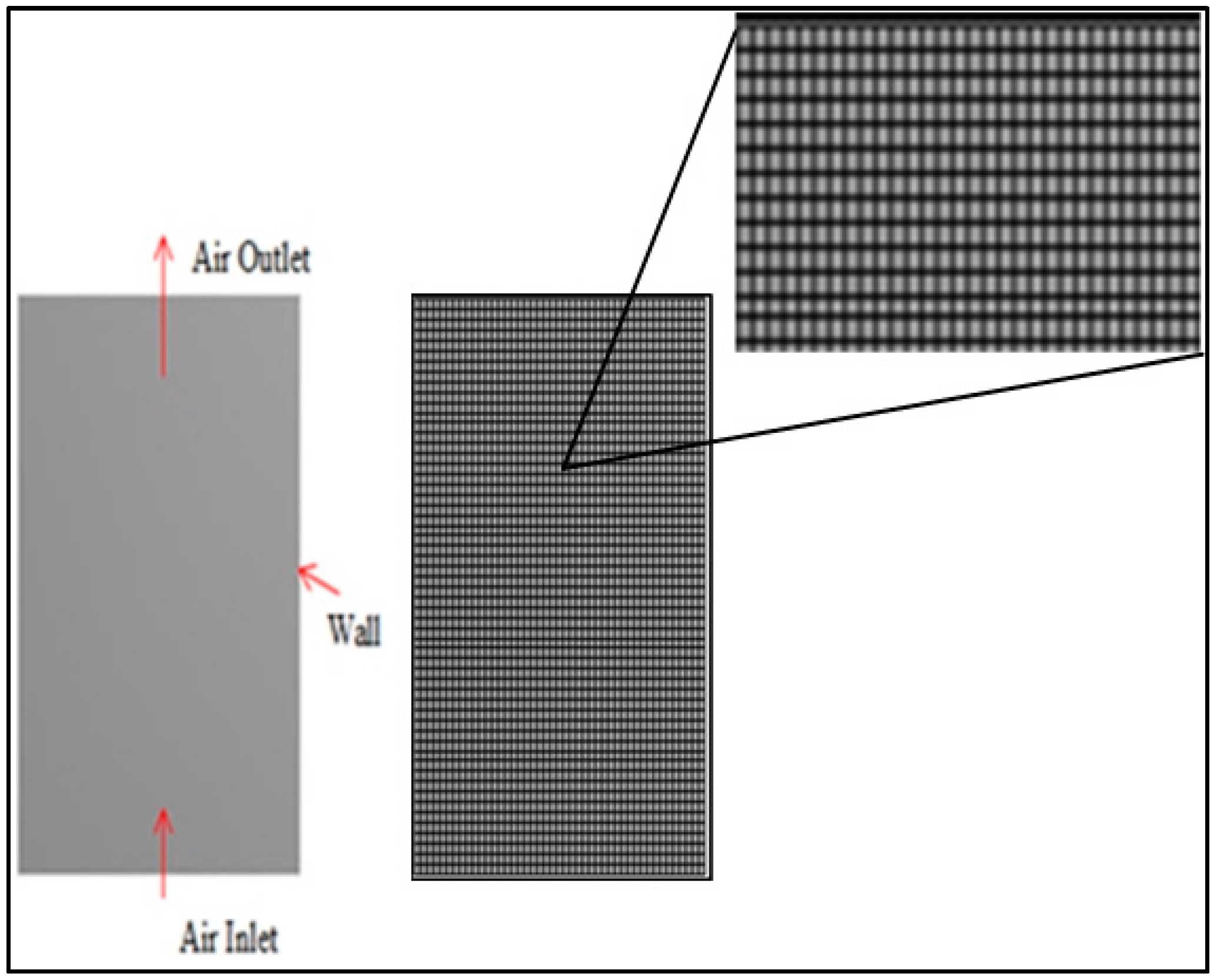
2.1. Development of Geometry and Mesh

The geometry dimensions for this work (0.22 m in height and 0.18 m in diameter) were borrowed from Ho [17] and constructed using ANSYS DesignModeler 17.1 (Ansys Inc., version 17.1, Canonsburg, PA, USA). The sago waste particles that were used as bed materials in the dryer had a height of 0.02283 m, which was calculated based on the density (1033 kg/m³) and mass (600 g) of sago waste in the experimental study.

A mesh independency test was conducted after developing the geometry. A fine mesh with 5141 elements and a minimum size of 0.039672 mm was used. Figure 1 shows the result of the meshing process.

2.2. Assumptions

Some assumptions were made for the simulation:

• No chemical reaction takes place in the drying process.
• The gas and solid are well-mixed.
• No slip conditions are set.
• The sago waste has an initial moisture content of 40%, as this is the suitable range of moisture content inlet for drying in a fluidized bed dryer.
• The sago waste does not agglomerate at a moisture content of 40%.
• The desired final moisture content of sago waste at the fluidized bed dryer outlet is selected to be 10% to preserve the nutrients of the sago waste [18].
• Particle size is not reduced with drying time and the different particle sizes are classified based on Geldart theory.
• The thermal properties of sago are assumed to be the same as those of cassava.

2.3. Modeling

The Eulerian–Eulerian multiphase model is used in this study because this tool requires less computational effort and is widely used in FBDs for CFD modeling. This model is composed of the air as the gas phase and sago waste as the solid phase. The heat transfer model is activated to analyze the heat transfer at the gas and solid regions in the model. A turbulence model is also employed due to the turbulent flow in the dryer. The standard k-ε model is also activated due to its simplicity and minimal computational requirements. In order to obtain the moisture ratio, model two-term exponential is inserted as a user-defined function.

2.4. Governing Equation

The conservations of mass and momentum are the main equations considered in the multiphase model. The conservation of energy and the equations in the turbulence model must also be considered for the heat transfer and the turbulence flow.

Conservation of mass [19]:

$$\frac{\partial }{\partial t}\left({\alpha }_q{p}_q\right)+\nabla \cdot \left({\alpha }_q{p}_q{\overrightarrow{v}}_q\right)={\displaystyle \sum _{p=1}^{\mathrm{n}}}\left({\dot{\mathrm{m}}}_{pq}-{\dot{\mathrm{m}}}_{qp}\right)+Sq$$

(1)

where:

• ${\overrightarrow{v}}_q$ = velocity of q phase;
• ${\dot{\mathrm{m}}}_{pq}$ = mass transfer from p^th phase to q^th phase;
• ${\dot{\mathrm{m}}}_{qp}$ = mass transfer from q^th phase to p^th phase.

Conservation of momentum [19]:

$$\begin{array}{l}\frac{\partial }{\partial \mathrm{t}} \left({\alpha }_q{p}_q{\overrightarrow{v}}_q\right)+ \nabla \cdot \left({\alpha }_q{p}_q{\overrightarrow{v}}_q{\overrightarrow{v}}_q\right)\\ =-{\alpha }_q\nabla p+\nabla \cdot {\stackrel{=}{\tau }}_q+{\alpha }_q{p}_q\overrightarrow{g}+{\displaystyle \sum _{p=1}^n}({\overrightarrow{R}}_{pq}+{\dot{\mathrm{m}}}_{pq}{\overrightarrow{v}}_{pq}-{\dot{\mathrm{m}}}_{qp}{\overrightarrow{v}}_{qp})+({\overrightarrow{F}}_q\\ +{\overrightarrow{F}}_{lift,q}+{\overrightarrow{F}}_{wl,q}+{\overrightarrow{F}}_{vm,q}+{\overrightarrow{F}}_{td,q})\end{array}$$

(2)

$${\stackrel{=}{\tau }}_q={\alpha }_q{𝓊}_q\left(\nabla {\overrightarrow{v}}_q+\nabla {\overrightarrow{v}}_q^T\right)+{\alpha }_q\left({\lambda }_q-\frac{3}{2}{𝓊}_q\right)\nabla \cdot {\overrightarrow{v}}_q\stackrel{=}{I}$$

(3)

where:

• ${\stackrel{=}{\tau }}_q$ = q^th phase shear stress tensor;
• ${𝓊}_q$ = shear viscosity of q phase;
• ${\mathsf{\lambda }}_q$ = bulk viscosity of q phase;
• ${\overrightarrow{ F}}_q$ = external body forces;
• ${\overrightarrow{F}}_{lift,q}$ = lift forces;
• ${\overrightarrow{F}}_{wl,q}$ = wall lubrication forces;
• ${\overrightarrow{F}}_{td,q}$ = virtual mass and turbulent dispersion forces;
• ${\overrightarrow{R}}_{pq}$ = interaction force between phases;
• p = pressure shared by all phases.

Conservation of energy [19]

$$\begin{array}{l}\frac{\partial }{\partial t} \left({\alpha }_q{p}_q{h}_q\right)+\nabla .\left({\alpha }_q{p}_q{\overrightarrow{u}}_q{h}_q\right)\\ = {\alpha }_q\frac{\partial p_q}{\partial t}+{\stackrel{=}{\tau }}_q:\nabla {\overrightarrow{u}}_q-\nabla .{\overrightarrow{q}}_q+S_q+{\displaystyle \sum _{p=1}^n}(Q_{pq}+{\dot{\mathrm{m}}}_{pq}{h}_{pq}-{\dot{\mathrm{m}}}_{qp}{h}_{qp})\end{array}$$

(4)

where:

• $h_q$ = specific enthalpy of q^th phase;
• ${\overrightarrow{q}}_q$ = heat flux;
• S_q = source of enthalpy;
• $Q_{pq}$ = intensity of heat exchange between p^th and q^th phases;
• $h_{pq}$ = interphase enthalpy.

Transport equation [19]:

$$\frac{\partial }{\partial t}\left(\rho k\right)+\frac{\partial }{\partial x_i}\left(\rho k{u}_i\right)=\frac{\partial }{\partial x_j}\left[(u+\frac{u_t}{{\sigma }_k})\frac{\partial k}{\partial x_j}\right]+G_k+G_b-\rho ϵ-Y_M+S_k$$

(5)

$$\frac{\partial }{\partial t}\left(\rho ϵ\right)+\frac{\partial }{\partial x_i}\left(\rho ϵu_i\right)=\frac{\partial }{\partial x_j}\left[(u+\frac{u_t}{{\sigma }_{ϵ}})\frac{\partial ϵ}{\partial x_j}\right]C_{1ϵ}\frac{ϵ}{k}\left(G_k+C_{3ϵ}{G}_b\right)-C_{2ϵ}\rho \frac{{ϵ}^2}{k}+S_{ϵ}$$

(6)

where:

• $G_k$ = generation of turbulence kinetic energy due to mean velocity gradients;
• $G_b$= generation of turbulence kinetic energy due to buoyancy;
• $Y_M$ = contribution of the fluctuating dilatation in compressible turbulence to overall rate;
• $C_{1ϵ}$, $C_{2ϵ}$, and $C_{3ϵ}$ = constants;
• $S_{ϵ}$, $S_k$= user source term.

Model two-term exponential:

$$MR=\mathrm{aexp}\left(-kt\right)+\left(1-a\right)\exp \left(-kat\right)$$

(7)

$$k=4.882\times {10}^{-4}T+1.506\times {10}^{-3}v-2.23\times {10}^{-3}$$

(8)

where;

• MR = moisture ratio;
• k = drying constant;
• T = air temperature;
• $v$ = air velocity;
• t = drying time (min);
• a = constant = 2.0888 [17].

2.5. Operating and Boundary Conditions

The gravitational acceleration was set to 9.81 m/s for the operating condition. Moreover, the inlet velocity of 1.30 m/s, temperature of 50 °C, and particle size of 2000 μm were used as boundary conditions. The inlet velocity of solid was set to 0 m/s to fix the bed in its original position. A no-slip condition was also set for the wall. The solid used in the simulation had a volume fraction of 0.45 [13]. The pressure outlet was also selected to reduce the reversed flow during the simulation.

2.6. Solution Procedure

The governing equations were solved by choosing the appropriate boundary conditions. The first-order implicit was selected; this is considered sufficient for the transient formulation in most problems. The first-order upwind was used in the spatial discretization for the convective terms except for the momentum, whilst the second-order upwind was used to improve the convergence. The phase-coupled semi-implicit method for pressure-linked equations (SIMPLE) was used for pressure velocity coupling in the multiphase model. A time step value of 0.075 s was also used to guarantee the stability of each simulation. Each simulation was run for 1 h with 48,000 time steps.

3. Results and Discussion

3.1. Validation of the Model

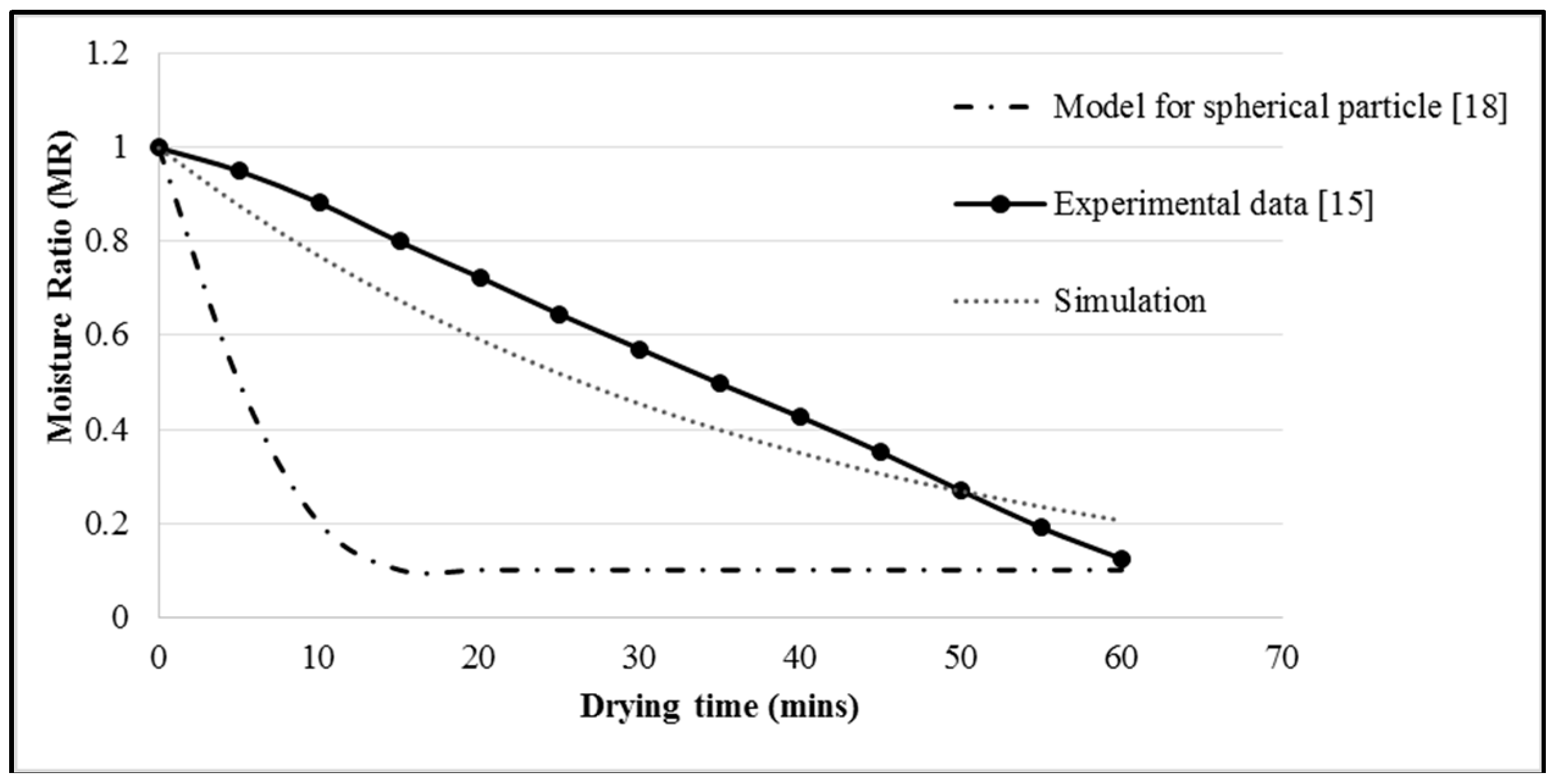
The model was validated by comparing the simulation results with the experimental findings of Ho (2016) [17] at an inlet air velocity of 1.30 m/s, inlet air temperature of 50 °C, and particle size of 2000 μm. The simulation results of this two-term exponential model were also compared with the simulation results of Zahir (2016) [20], as shown in Figure 2. Both the simulation and experimental data curve showed a diverse trend with the spherical particle data due to the different utilizations of the tool and model by the researcher. The simulation curve exhibited the same trend as the experimental data, thereby generating a minimal number of errors in the comparison. This simulation work also showed an improved prediction of the drying profile for sago waste compared to the simulation work performed by Zahir using a model of spherical particles.

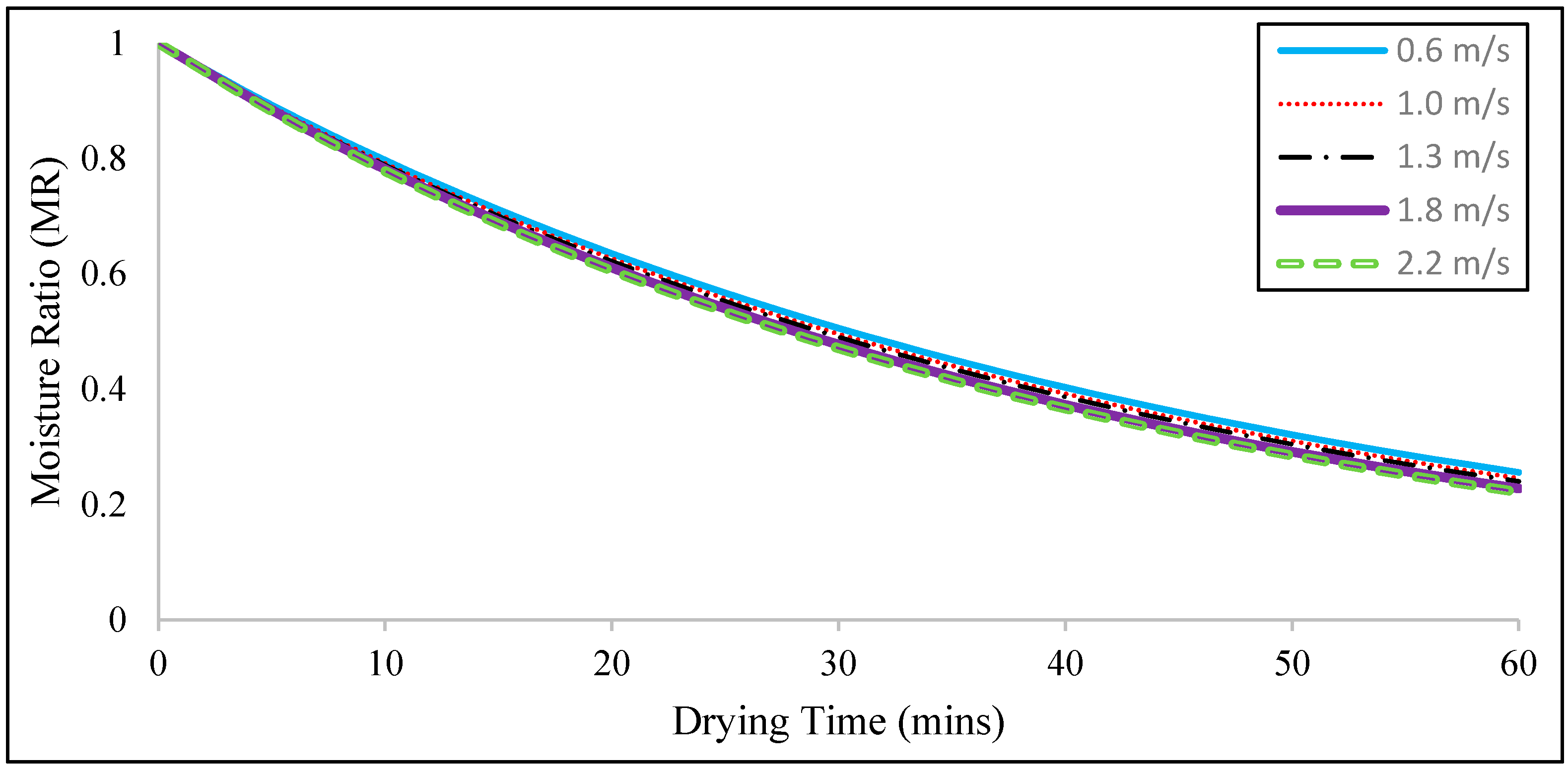
3.2. Effect of Air Velocity on CFD Modeling Performance

Figure 3 shows that the moisture ratio curve continuously decreases with time. Meanwhile, the drying time it takes to achieve a final moisture ratio of 0.25 decreases along with increasing air velocity. The shortest required drying time (56 min) is recorded at a peak velocity of 2.2 m/s but exceeds 1 h at a velocity of 0.6 m/s. This finding can be ascribed to the fact that a higher heat transfer rate is recorded at higher velocities. Specifically, the drying time reaches 59, 58, and 57 min at velocities of 1.0, 1.3, and 1.8 m/s, respectively. These results clearly indicate that velocity does not have any significant effect on the moisture ratio curve because the differences amongst the drying times recorded at velocities of 1.0, 1.3, 1.8, and 2.2 m/s are only 1 min at most. This finding may be attributed to the fact that the considered velocity range is not large enough to produce an obvious effect.

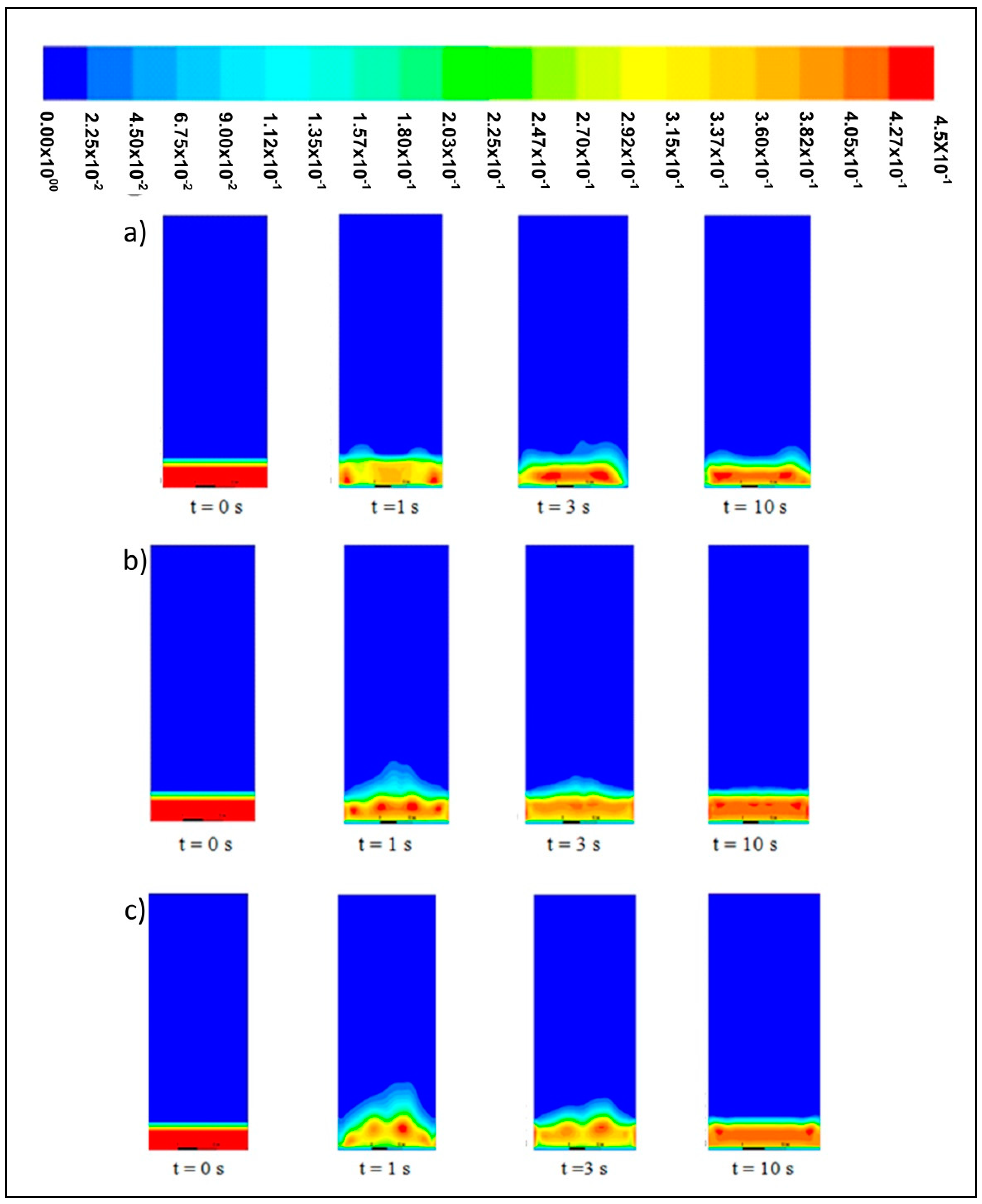
Figure 4 shows the solid volume fraction contour at different velocities. These contours exhibit the same trends across different bed heights in a simulation time range of 0 s to 10 s.

At 0 s, the solid bed is fixed at a height of 0.02283 m with a velocity of 0 m/s. This bed starts to fluidize at 1 s and demonstrates a fluid-like behavior when the inlet upward-flowing gas interacts with the particle bed. The drag force, which refers to the frictional force imposed by the inlet air and downward gravitational force, is addressed. At the initial stage, the bed expands rapidly until reaching its maximum height. At a velocity of 0.6 m/s, both fluidization and bed expansion are kept at minimal levels, whereas the recorded bed height is almost the same as its initial level.

The particles with a size of 2000 μm undergo bubbling fluidization at velocities of 1.0, 1.3, 1.8, and 2.2 m/s. At 1 s, these particles move upwards along with inlet gas in the central position of the bed. Afterwards, the bed rapidly expands because the movement of bubbles from the bottom to the top of the bed will distribute the particles along the bed height. At velocities of 1.0 m/s and 1.3 m/s, a small bubbling fluidization is observed at the initial stage, whilst at velocities of 1.8 m/s and 2.2 m/s, a large bubbling fluidization is observed and results in the further expansion of the bed.

At 3 s, the bed region is flattened as the bed height decreases from the level recorded at 1 s. According to Verma et al. [21], the reduction in bed height before the flattening of the bed region could be ascribed to the formation of huge bubbles at 1 s.

At 10 s, the bed region is flattened at each velocity and remains in its flat state despite the increase in bed height.

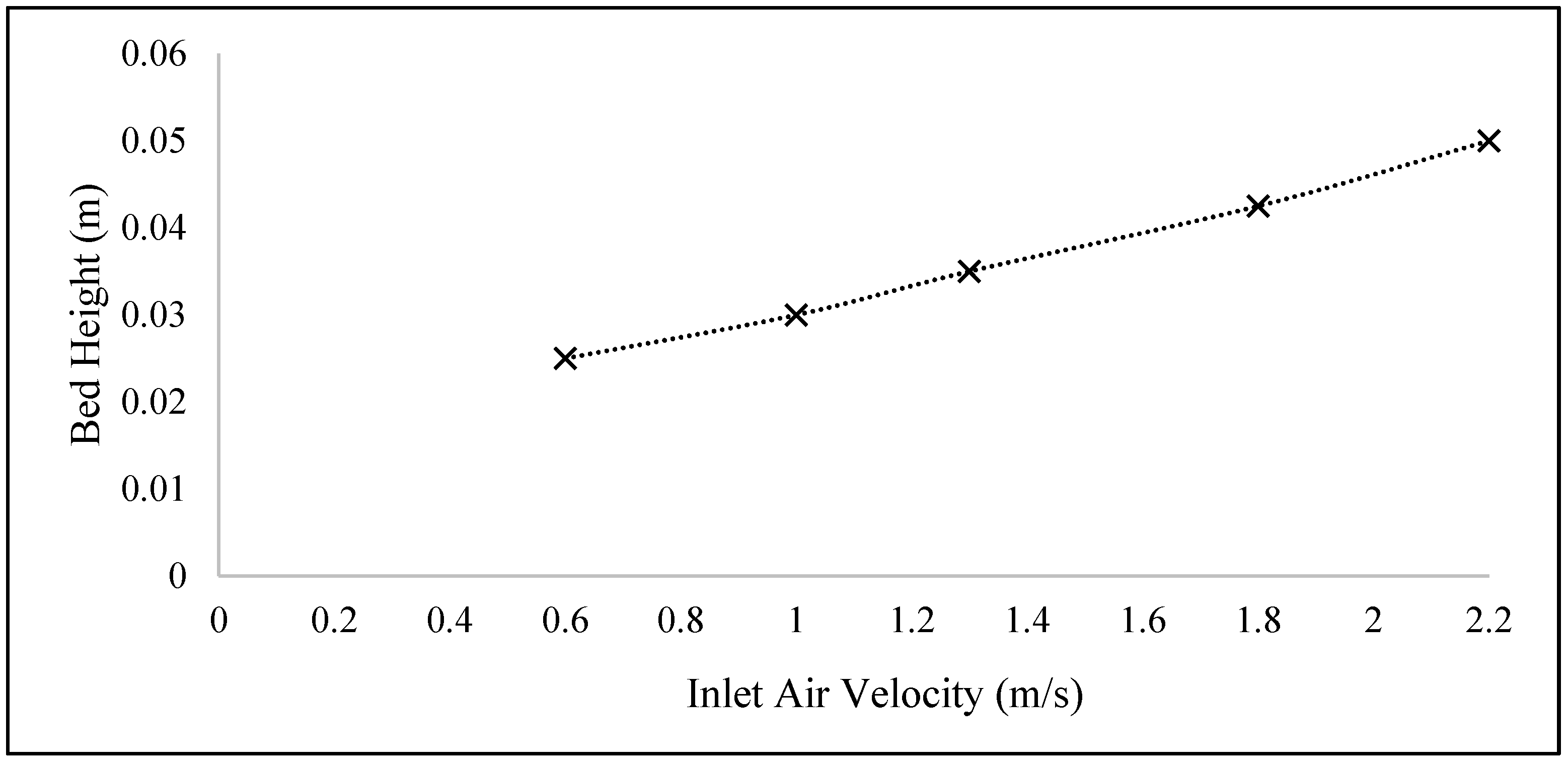
Figure 5 shows that the bed height reaches 0.025, 0.03, 0.035, 0.0425, and 0.05 m at velocities of 0.6, 1.0, 1.3, 1.8, and 2.2 m/s, respectively. At each velocity, the bed height slightly increases from its initial level of 0.00283 m because those particles with a size of 2000 μm cannot be easily fluidized according to Geldart theory.

Higher velocities can be set to achieve a shorter drying time and favorable fluidization for particles with a size of 2000 μm. However, setting high velocities may result in the entrainment of all particles outside of the bed. Thus, the air velocity has a more significant effect on fluidization compared to the drying rate. The results showed that a velocity range of 1.0 m/s to 2.2 m/s rendered the particles with a size of 2000 μm able to fluidize.

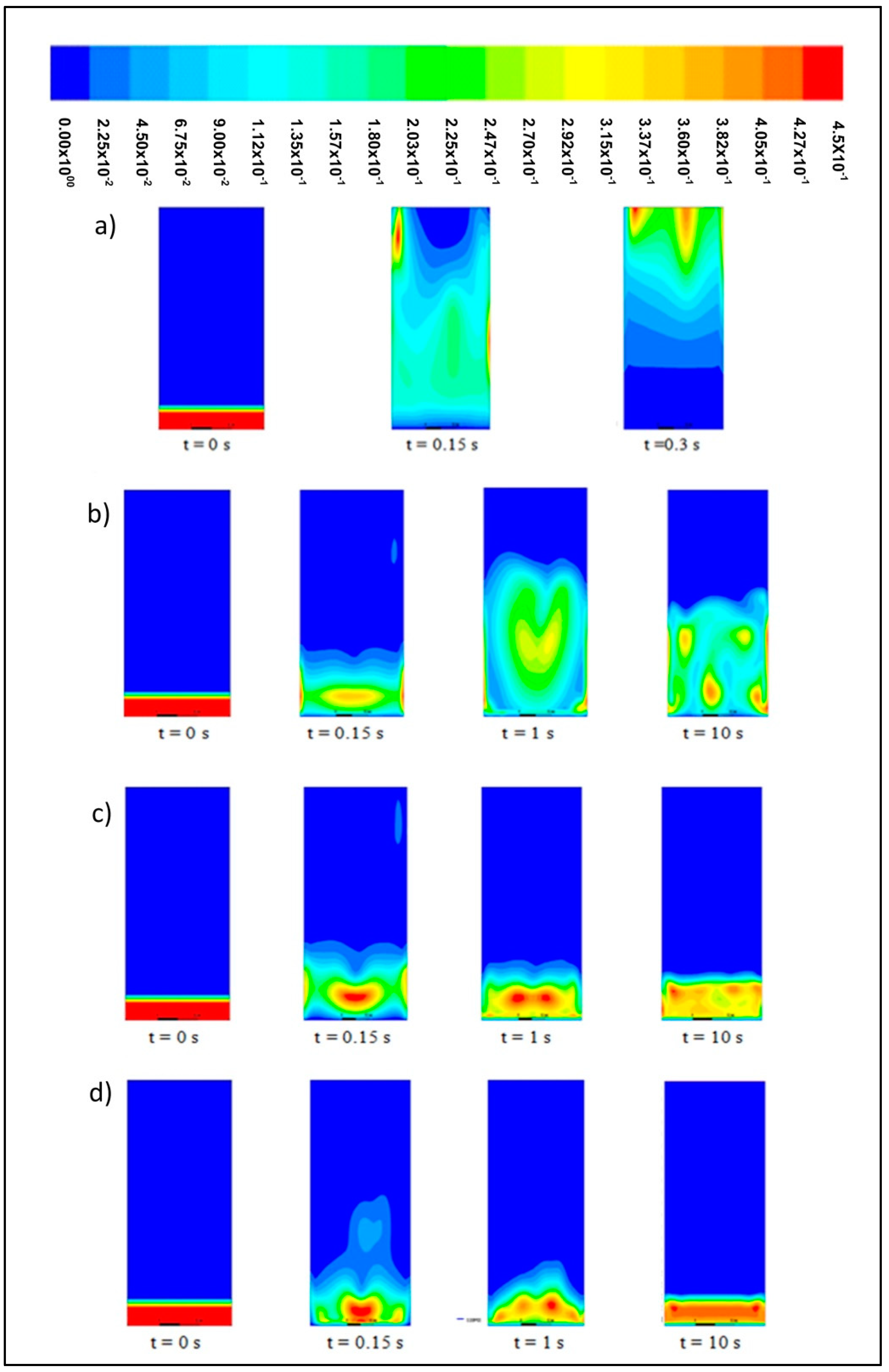
3.3. Effect of Particle Size on CFD Modeling Performance

The effects of particle sizes 200, 500, 1000, and 2000 μm on the contour solid volume fraction are shown in Figure 6. These contours are divided into two phases, where the red color represents the solid phase with a volume fraction of 0.45, while the blue color represents the air phase with a volume fraction of 0. Sago has a density of 1033 kg/m³. Moreover, according to Geldart theory [22], those particles with sizes of 200, 500–1000, and 2000 μm are classified into groups A, B, and D, respectively. Particle group C with a size range of 10–20 μm was not included since it is not suitable to be used in FBD and shows poor fluidization [23].

In Figure 6a, it is shown that rapid fluidization takes place at 0.15 s and that the fluidization process continues until all particles are entrained out of the bed at 0.3 s. Entrainment of the solid particles causes a loss in particles mass. The inlet gas also continues to impose a very high drag force until the equal and opposite drag forces imposed by the particles are fully overcome.

The largest bed expansion is observed amongst particles with a size of 500 μm, as seen in Figure 6b. In this case, the fluidization begins at 0.15 s and the bed further expands at 1 s due to the behavior of the particles in group B, which are easily fluidized. According to Geldart [22], the particles in this group often undergo bubbling fluidization rather than smooth fluidization. Given that bubbles are formed at the beginning of the fluidization at 0.15 s, the minimum bubbling velocity is the same as the minimum fluidization velocity.

In Figure 6c, similar findings are observed for those particles with a size of 1000 μm, which are also classified under group B. Meanwhile, the bed only shows a minimal expansion for those particles with a size of 500 μm because at a velocity of 1.3 m/s, these particles show a less smooth fluidization compared with the other particles. Those particles with a size of 2000 μm (group D) undergo bubbling fluidization with minimal bed expansion. Moreover, the formed bubbles are unable to reach their maximum size and tend to fall back to the lower bed height after 10 s. These particles also show a poor fluidization compared with the particles in group B.

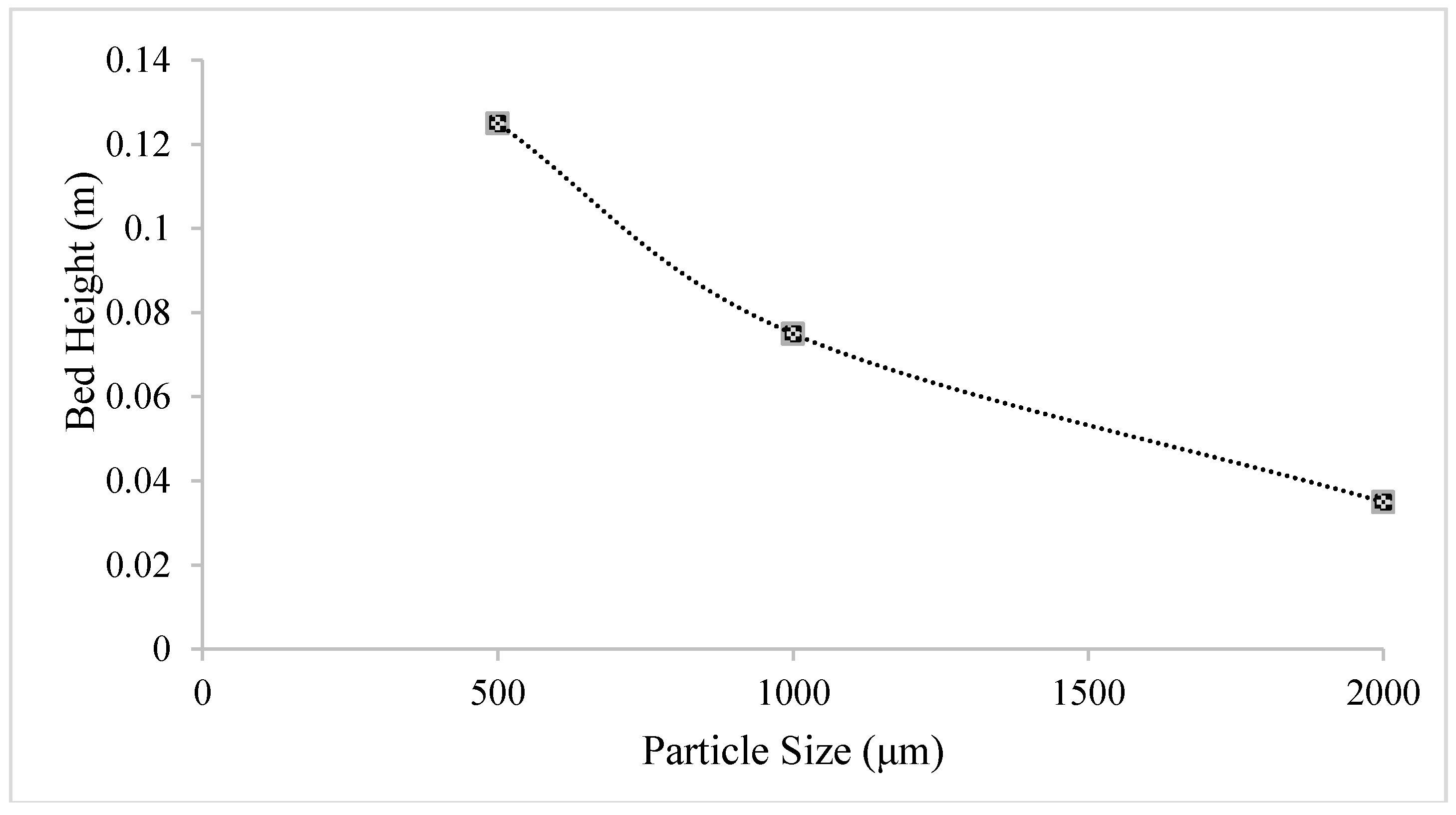
Figure 7 shows the expansion of the bed across different particle sizes from its initial height of 0.02283 m. A smaller particle size shows a greater bed expansion because small particles can be easily fluidized. However, fluidization also depends on air velocity, as can be observed in the fluidization of particles with a size of 200 μm. As can be seen in Figure 7, those particles with sizes of 500, 1000, and 2000 μm demonstrate the greatest bed expansions of 0.125, 0.075, and 0.035 m, respectively. The bed height for 200-μm particles was excluded as the value of the bed during fluidization exceeded the height of the dryer. Therefore, at a velocity of 1.3 m/s, the ideal particles for the fluidization had a size range of 500 μm to 2000 μm. The particles in group B exhibited better fluidization than those in group D. The particles in group A are not recommended for the velocity of 1.3 m/s because such a velocity will entrain all these particles out of the bed.

4. Conclusions

A simulation was performed to examine the influence of inlet air velocity, inlet air temperature, and particle size on achieving the final moisture ratio of 0.25. The multiphase Eulerian model was used to describe the gas–solid turbulent flow. A 2D CFD model with a fine mesh was also developed. The small errors in the model validation indicated that this model is acceptable. The optimum parameters (i.e., 1.3 m/s, 50 °C, and 2000 μm) from the experiment of Ho. Y.N [17] were used as the base case for analyzing these parameters further.

The moisture ratio curve and fluidization profile for particles with a size of 2000 μm were analyzed at air velocities of 0.6, 1.0, 1.3, 1.8, and 2.2 m/s and at a temperature of 50 °C. Increasing the air velocity shortens the required drying time to achieve the desired final moisture ratio. However, the effect of air velocity on the drying curve is less significant than that of the fluidization profile. An air velocity of 1.0 m/s to 2.2 m/s was found to be suitable for the fluidization of particles with a size of 2000 μm.

The inlet air temperatures of 50, 60, 70, and 80 °C were manipulated at 1.3 m/s for those particles with a size of 2000 μm. The results indicated that the final moisture content can be achieved within a short drying time at a high air temperature. Such a temperature also results in a high heat transfer and drying rate.

Different fluidization patterns were observed for particles with sizes of 200, 500, 1000, and 2000 μm at a velocity of 1.3 m/s and temperature of 50 °C. A smaller particle size also leads to a greater bed expansion. However, such an expansion also depends on the air velocity. Those particles with a size range of 500 μm to 2000 μm were found to be able to undergo fluidization at 1.3 m/s.

Some improvements need to be implemented to obtain better and more accurate results. Given that only a few studies have examined the drying of sago waste, further experiments must be conducted to determine the thermodynamic and thermal properties of these materials. A more complex CFD model that includes both the evaporation of sago moisture into inlet air and the mass and moisture transfer must also be employed in future studies. The interaction process may also require the utilization of a user-defined function code.