Article

Function Value-Based Multi-Objective Optimisation of Reheating Furnace Operations Using Hooke-Jeeves Algorithm

1
School of Information Science and Engineering, Central South University, Changsha 410083, China
2
Complex Systems, School of Management, Cranfield University, Bedford MK43 0AL, UK
3
Faculty of Computing, Engineering and Science, University of South Wales, Pontypridd CF37 1DL, UK
*
Author to whom correspondence should be addressed.
Energies 2018, 11(9), 2324; https://doi.org/10.3390/en11092324
Submission received: 14 August 2018 / Revised: 28 August 2018 / Accepted: 30 August 2018 / Published: 3 September 2018

Abstract

:
Improved thermal efficiency in energy-intensive metal-reheating furnaces has attracted much attention recently in efforts to reduce both fuel consumption, and CO2 emissions. Thermal efficiency of these furnaces has improved in recent years (through the installation of regenerative or recuperative burners), and improved refractory insulation. However, further improvements can still be achieved through setting up reference values for the optimal set-point temperatures of the furnaces. Having a reasonable expression of objective function is of particular importance in such optimisation. This paper presents a function value-based multi-objective optimisation where the objective functions, which address such concerns as discharge temperature, temperature uniformity, and specific fuel consumption, are dependent on each other. Hooke-Jeeves direct search algorithm (HJDSA) was used to minimise the objective functions under a series of production rates. The optimised set-point temperatures were further used to construct an artificial neural network (ANN) of set-point temperature in each control zone. The constructed artificial neural networks have the potential to be incorporated into a more advanced control solution to update the set-point temperatures when the reheating furnace encounters a production rate change. The results suggest that the optimised set-point temperatures can highly improve heating accuracy, which is less than 1 °C from the desired discharge temperature.

1. Introduction

The iron and steel industry, combined, is energy-intensive. According to statistical data, reported by the International Energy Agency, this industry accounted for 18% of total industry final energy consumption of the entire word in 2013 [1], and their analysis of 2012 highlights that applying the best available technology has potential to reduce about 20% of current total energy consumption [2]. Metal reheating is one of the most energy intensive processes within the iron and steel industry [3], accounting for 15–20% of the total energy consumption of the industry. In this process, intermediate steel products such as blooms (known as stock) which are also called billets or slabs are heated to a specific temperature and through-thickness temperature uniformity before hot-rolling [4]. Due to the variabilities in furnace operation (which may include changes in the stock dimension and/or metallurgical grade, and the production rate) inconsistency in the quality of the final heated product can sometimes occur, resulting in unnecessary rejects. It has been estimated that a reduction of rejects from 1.5% to 0.2% could lead to energy savings of up to 9% of energy consumption or approximately 0.3 GJ/tonne-product [5]. To operate the reheating furnace efficiently while supplying products of a consistent quality, it is necessary to implement an effective furnace-temperature control strategy.
With the continued development of computer technology, computing power is increasingly affordable. The numerical simulation of steel reheating furnaces, which depends on the actual physics of the working process and then builds approximate mathematical models [6,7,8,9,10], has become widely used as a cost-effective and powerful engineering tool. These numerical simulations can be classified into two categories. The first category uses computational fluid dynamics (CFD) to solve the Navier–Stokes and energy conservation equations for the thermal radiative transport phenomena associated with hot gas flow and combustion processes in a furnace [11,12,13,14]. Although these CFD mathematical models make it possible to depict the whole furnace including the temperature distribution of the stock in each position, the quality of simulation results depends strongly on the size and density of computational grid the employed, leading to long processing times. Once the models are constructed, the CFD simulation cannot be used for a dynamic control system, due to the length of time required for iterative computation.
Simulation methods in the other category, based on the zone method of radiation analysis [15], analyse the radiative heat transfer within the furnace and transient heat conduction in the slabs [6,9,16,17]. This approach does not require the degree of computing power associated with CFD, and even a consumer-level computer can run the zone model code quite quickly [6]. Although reactive flows are ignored in this approach, the simulation results are sufficiently accurate for studying the temperature control of the furnace [18]. The authors note that the main purpose of this paper is to reliably obtain the optimisation reference set-point temperatures for a temperature controller. Therefore, this second category of simulation methods is suitable here for the accurate modelling of the thermal behaviour of the slabs.
Set-point temperatures are important for any furnace, as these are used by the control system to adjust the fire rates of burners to achieve the desired temperature profile of the stock. However, the temperature profile desired varies according to many factors, including the dimension and material properties of the slab, as well as the throughput rate of the furnace. Unfortunately, the methods used for determining necessary set-point temperatures to achieve desired temperature profiles, in specific furnace operations, are rarely published. To the authors’ knowledge, there are two papers based on the zone method of radiation analysis which detail the optimisation of set-point temperatures. The first one solves the partial differential equation (PDE) optimal control problem to obtain set-point temperatures by introducing the adjoint problem to the optimization model [18]. Although this paper reports some remarkable results, in comparison to the use of the finite difference method, the method is tailored to an atypical control system which may be invalid for other furnaces. The second paper uses a genetic algorithm (GA) based on a multi-objective optimisation strategy to optimise temperature trajectory of the bloom by minimising a cost function. The cost function has been built by a set of fuzzy rules and it adapts easily to different furnace operations [19]. It also reports impressive results, and has the benefit that this optimisation strategy is a common method and is therefore suitable for any other furnaces. Hence why this second approach has much more potential for broad application. That noted, however, GA approaches are prone to premature convergence to local optima of the objective function [20], making it difficult to ascertain whether a solution obtained is actually the desired global optimum. And also note that it is technically impossible to identify a global minimum unless the feasible region is shown to be convex. Therefore, one of the purposes of this paper is to explore another common optimisation method, strongly underpinned by a mathematical framework, to make comparison with the GA approach to determine which one has a better performance (It is noted here that since the optimisation work using GA was performed by co-authors of this paper, the results are readily available for comparison; see Section 4 for more details.).
In this paper, a function values-based multi-objective optimisation is presented to obtain desired set-point temperatures of a reheating furnace. The Hooke-Jeeves direct search algorithm (HJDSA) is chosen as the core technology for the multi-objective optimisation method presented [21]. This minimization algorithm uses function values only, and therefore it can be used to solve objective functions in most multi-objective problems. This paper presents an objective function which contains three dynamic parameters relating to energy consumption and product quality: Discharge temperature of blooms; maximum temperature difference in bloom cross section; and specific fuel consumption. In addition, two weighted factors are introduced into the function to match six different optimisation scenarios. The objective functions are solved by HJDSA to obtain the desired set-point temperatures.
For this HJDSA approach, the main computer program would require five hours to complete the necessary detailed calculation for a change in production rate. Evidently this does not meet the requirement of real time prediction of the furnace, and so for the timely and accurate prediction of set-point temperatures, one of the most well-known artificial neural networks (ANNs) [22,23] was introduced. As black-box models [24], ANNs are able to capture the non-linear processes underlying many problems, and hence they are widely used for optimisation problems [25]. Four back propagation neural networks [26] were constructed, trained, and tested using 37 datasets calculated by HJDSA under 37 different conditions within the range of lowest to highest production rates. After obtaining optimal training results, the four neutral networks were in turn input back into the program to replace the HJDSA module for other conditions with unseen production rates. The advantage of this approach is that the neural networks, when constructed on sufficient precise training data, can mimic the optimisation process of HJDSA while achieving results in in much shorter time. It is noted, however, that this may also be a weakness, because one of the input parameters of the neural networks should be adjusted manually to make sure the ΔTdis within ±5 °C. This manual processing contains a series of attempts that may take time.
The results suggest that the optimised set-point temperatures calculated by HJDSA can highly improve heating accuracy, which is less than 1 °C from the desired discharge temperature. Although the set-point temperatures predicted by neural networks have a poorer heating accuracy about 5 °C, it takes a few milliseconds to get the temperatures, which implies that real time simulation of zone model is successfully maintained when production rate changes.
The rest of the paper is organised as follows: Initially, Section 2.1 describes the structure of a furnace, the operation of it and its control system. Section 2.2 presents the optimisation algorithm of furnace operations. Based on the optimisation scenarios which are shown on Section 2.2.1, the Section 2.2.2. uses Hooke-Jeeves direct search algorithm to calculate optimised set-point temperatures under a series of production rates. Last, but not least, the optimised set-point temperatures were further used to construct an artificial neural network of set-point temperature in each control zone, as shown in Section 2.3. Section 3 and Section 4 present the results and discussion, respectively. Finally, Section 5 concludes the paper.

2. Materials and Methods

The structure of a certain furnace and its control system are firstly introduced in this part. Based on the furnace operation, different optimisation scenarios are then designed which consider the economic operation of the furnace and supply products of a consistent quality by three parameters. An objective function is thus built which contains the three parameters, and then solved by HJDSA in different optimisation scenarios to get desired set-point temperatures. Since the gradient information of the objective function is not available, the HJDSA is chosen as the core technology to solve the function. However, it takes almost 5 h for each scenario to obtain the desired set-point temperatures by HJDSA. This is a limitation of the zone model approach, making it incapable of real time prediction. To overcome this limitation, four back propagation neural networks are used for the determination of the four desired set-point temperatures eventually. In order to make the aforementioned process clearly and easy to understand, Figure 1 shows the steps of research of this study.

2.1. Furnace Operation and Control

The furnace studied is a large-scale walking-beam reheating furnace, which can be illustrated in Figure 2. There are total 71 burners installed in 6 control zones, and 2 slave zones are among them, i.e. zones 2 and 4 are slaves to zones 1 and 3, respectively. The energy inputs of the slave control zones are proportional to the energy inputs of the master control zones. That means this paper only need to optimise set-point temperature of control zone 1, 3, 5, and 6. Under monitoring and control, a sequence of blooms walks through all heating zones with a specified dynamic pace rate before they are discharged from the furnace for downstream processing.
The process control solution for the reheating furnace is shown in Figure 3. The zonal temperatures inside the furnace are controlled by set-points determined dynamically by a model-based level-2 module, thereby achieving the required quality of heating profile quality heating in various production scenarios. In operation, online monitors predict bloom temperatures using furnace wall temperatures measured by a limited number of thermocouples which are compared with a pre-specified bloom temperature profile, then feeding back set points to the temperature controller (e.g. PID control). This process control solution has been shown to be an effective way of achieving a consistent reheating process [6].

2.2. Optimisation Algorithm

Recent studies [6] have made a validity of zone model, which can simulate the heating conditions of blooms when they are moved through the furnace. That model employs the well-known zone method with a rigorous treatment of radiation, taking into consideration the full energy balance of the furnace. The computational efficiency of the zone model is remarkable, even with a consumer-level PC hardware, implying that the model has the ability of real time simulation and has great potential for using in parametric studies of furnace operations, which also could be using directly into dedicated furnace optimisation and control algorithms. Therefore, this model is used as a predictor in the multi-objective optimisation in this study.

2.2.1. Optimisation Scenarios

Considering the economic operation of the furnace and providing products of a consistent quality, there are three dynamic parameters accessed to them which are desired discharge temperature, maximum temperature difference in bloom cross section and specific fuel consumption. Based on this, several optimisation scenarios are taken into consideration which can be seen in Table 1. In all cases, the heating accuracy (ΔTdis) is given priority, because it is the primary target in any reheating process (the priority objective). Two other optimisation objectives are included: The maximum temperature difference in bloom cross section (ΔTmax), which is an improvement quality index for discharge blooms, and specific fuel consumption (SFC), which is closely connection with the distribution of thermal input along the length of the furnace, which in turn also influences on the profile of heating rates of a certain bloom as it moves through the furnace. These additional objectives are added singly (scenarios I and II), and together (scenario III), setting weighted factors M and N such that they are emphasized at the same objective level. The production rate also influences on the residence time of bloom, energy consumption and heating uniformity. Therefore, three similar scenarios are considered at a different production rate (scenarios IV to VI).

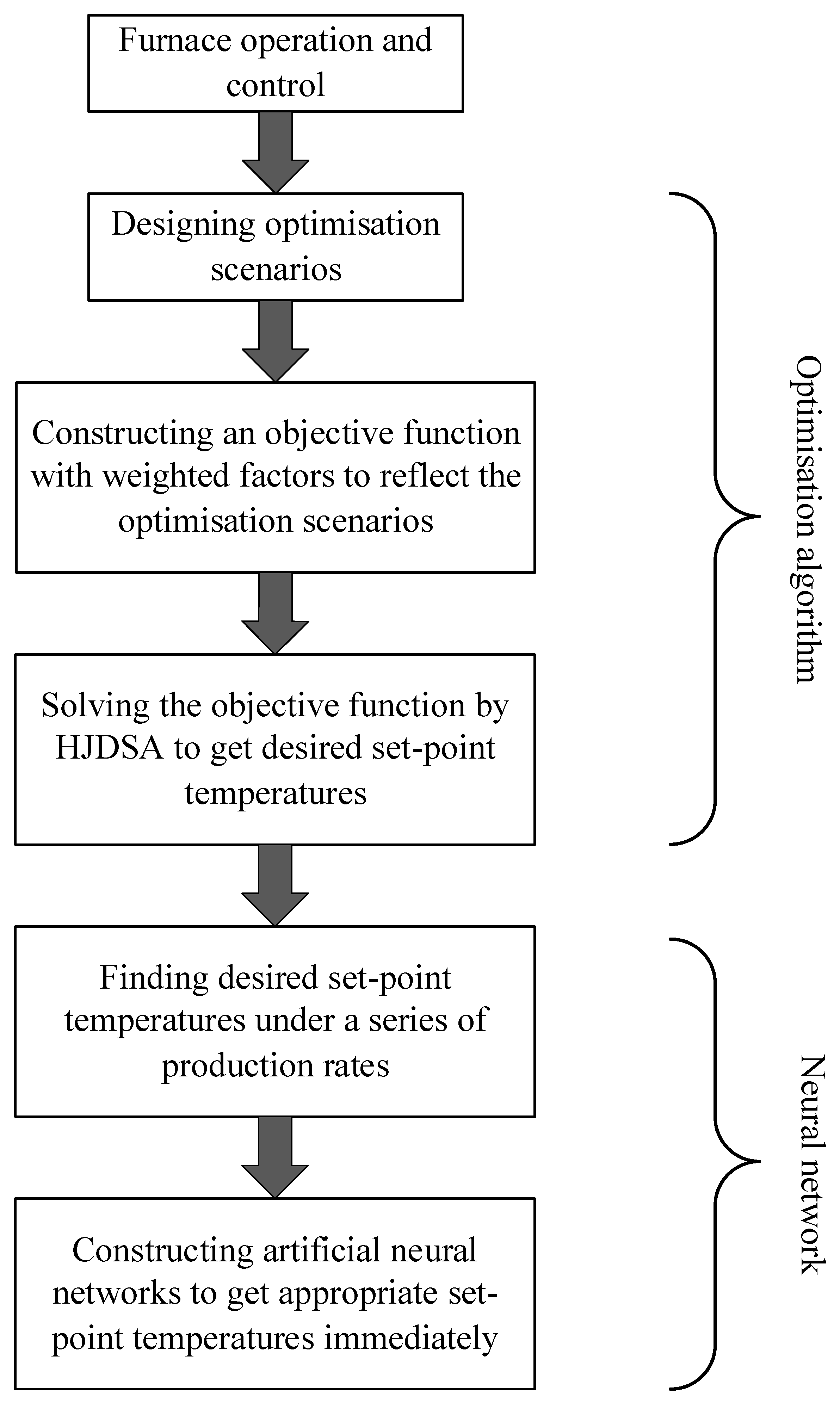
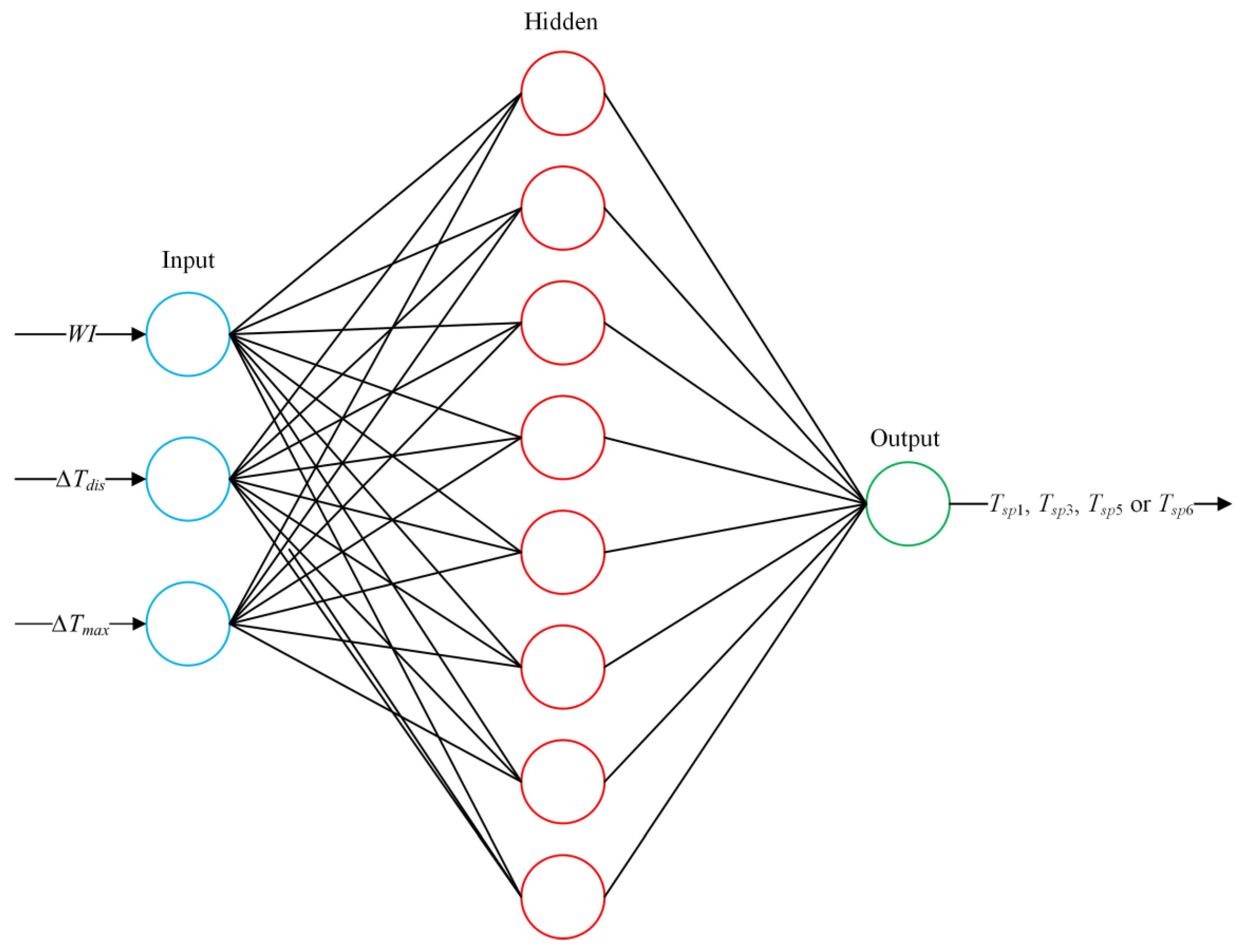
2.2.2. Hooke-Jeeves Direct Search Algorithm (HJDSA)

To solve the multi-objective optimisation problem in different furnace operations as shown in Table 1 by HJDSA, this part stage constructs an objective function step by step. The objective function then works like a bridge to build a connection between the zone model unit and the HJDSA unit. Throughout the optimisation process, parameters are passed continually between the units, ensuring the success of HJDSA in obtaining the desired set-point temperatures.
● The objective functions
In order to reveal the relationship of the three parameters affecting the economic operation of the furnace and the supply of products at a consistent quality, and to explore how set-point temperatures impact on them, an objective function is first built, and then solved by HJDSA [21] in different optimisation scenarios.
For several continuous drop-out blooms during a steady-state operation with the difference between the desired and the realistic discharge temperature ΔTdis and maximum temperature difference ΔTmax in bloom cross section, there is an objective function:
J = i = 1 n Δ T i d i s 2 + M i = 1 n Δ T i m a x 2 + N i = 1 n S F C i 2 ,
where n is the total number of blooms, ΔTidis is the difference between the desired and the real discharge temperature of bloom i, ΔTimax is maximum temperature difference in bloom i and SFCi is the specific fuel consumption at the moment of bloom i discharged, M and N are weighted factors.In this study, four adjacent drop-out blooms are taken into consideration after the furnace model running 5000 s, and the target discharge temperature is 1230 °C. Weighted factors M and N are taken from Table 1 in accordance with the different optimisation scenarios.
● Finding optimal set-point temperatures by HJDSA
In this study, the core algorithm used in the multi-objective optimisation is HJDSA, which searches for the minimizing point of a function f(x) of several variables by exploring desired values near initial set-point values. A gradient-based method may be more efficient, however many real-world optimisation problems require using computationally expensive simulation packages to get the result of the objective function, thus it is difficult to calculate the derivative of the objective function [27]. For the multi-objective optimisation problem in this paper, the objective function takes into consideration the discharge temperature and maximum temperature difference in bloom cross section. Since these two parameters relate to different discharge blooms, the objective function is not continuous and therefore not differentiable, which means the gradient information of the function is not available. Hence, direct search techniques must be used instead. The HJDSA algorithm does not require the function f(
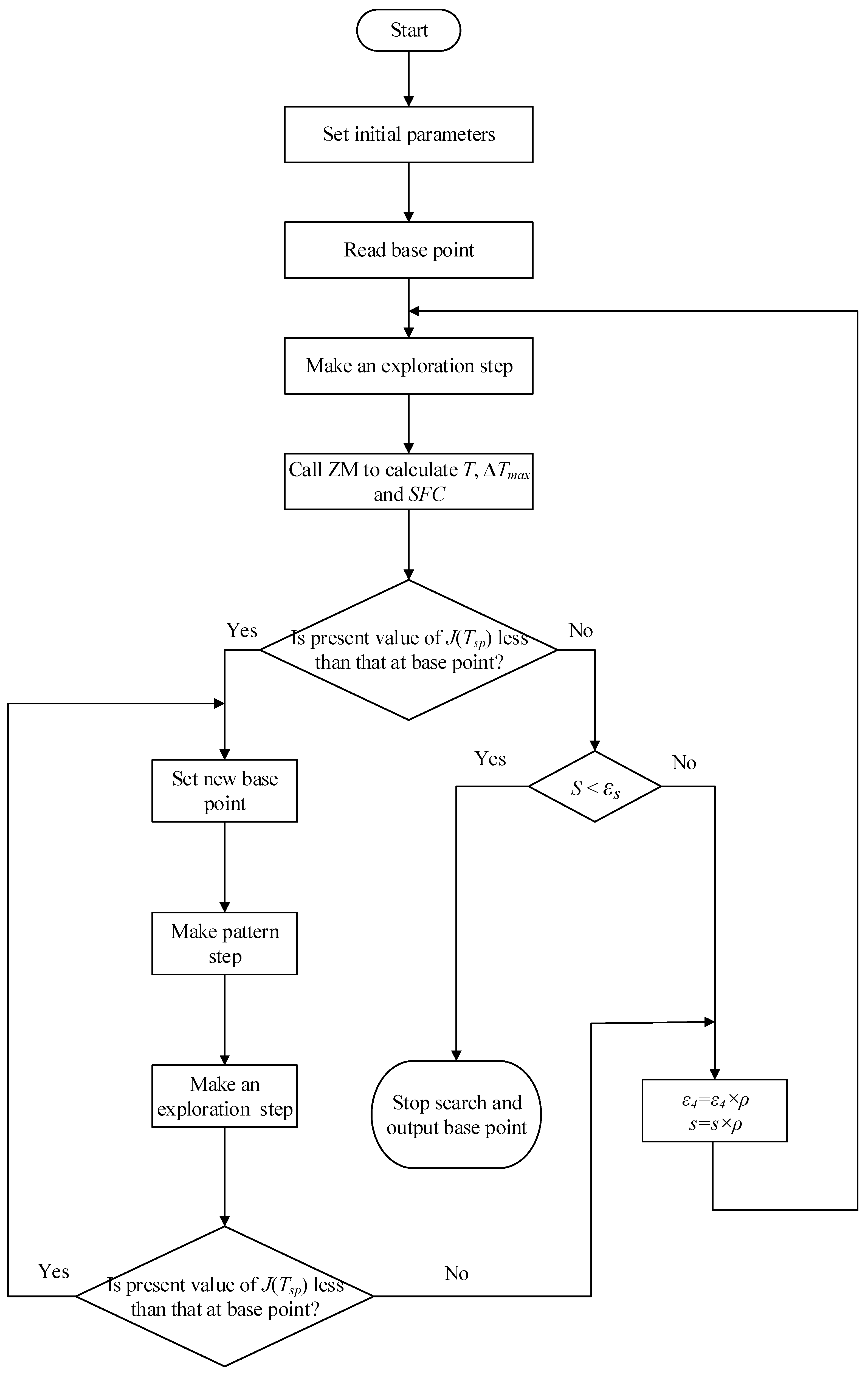
x) to be differentiable nor even to be continuous, as it only examines function values and remembers the location of the best value encountered, seeking to improve this value by a pattern search. This pattern search consists of a sequence of exploratory moves about a base point, with and pattern moves being followed if the exploratory moves fail to improve the objective function.
An exploratory move is made to get information about the function f(x) near the current base point ak (ak = (x1, x2, …, xi)). Each variable xi is firstly set an increment εi in the positive direction of xi and then in the negative direction, and after each move there is a check for the new function value. If a move results in a smaller function value, then the new value of that variable will be remained. After all the variables have been taken into consideration, a new base point ak+1 will be reached. If ak+1 = ak, the function f(x) has no reduction, and the increment εi is reduced, repeating the above process. If ak+1ak, a pattern move from ak is made.
A pattern move, using information already obtained about f(x), is made to determine the best search direction in an attempt to hasten the search. A move from ak+1 is made in this direction ak+1ak, as a move in the direction has led to reduce the function value. Hence the next pattern point is given by following equation [27]:
b k = a k + 1 + ( a k + 1 a k ) .
The search then continues with a new series of exploratory moves about bk, and if the minimum function value achieved is less than f(ak), then a new base point ak+2 has been achieved. If not, the pattern from ak+1 is abandoned and the search continues with a new set of exploratory moves about ak+1. The minimum is assumed to be achieved if the step length s has been decreased to a specified small value εs.
Overall, a direct search for the minimizing point of a function by Hooke-Jeeves algorithm employs variables not directly referred to in Equation (1). Therefore, Equation (1) is rewritten as follows:
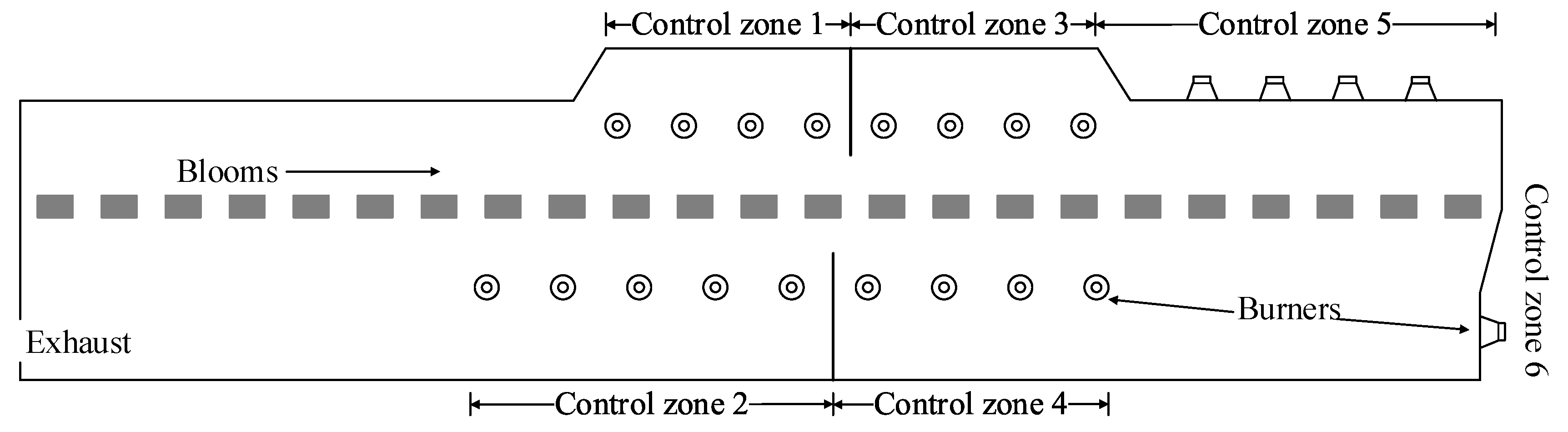
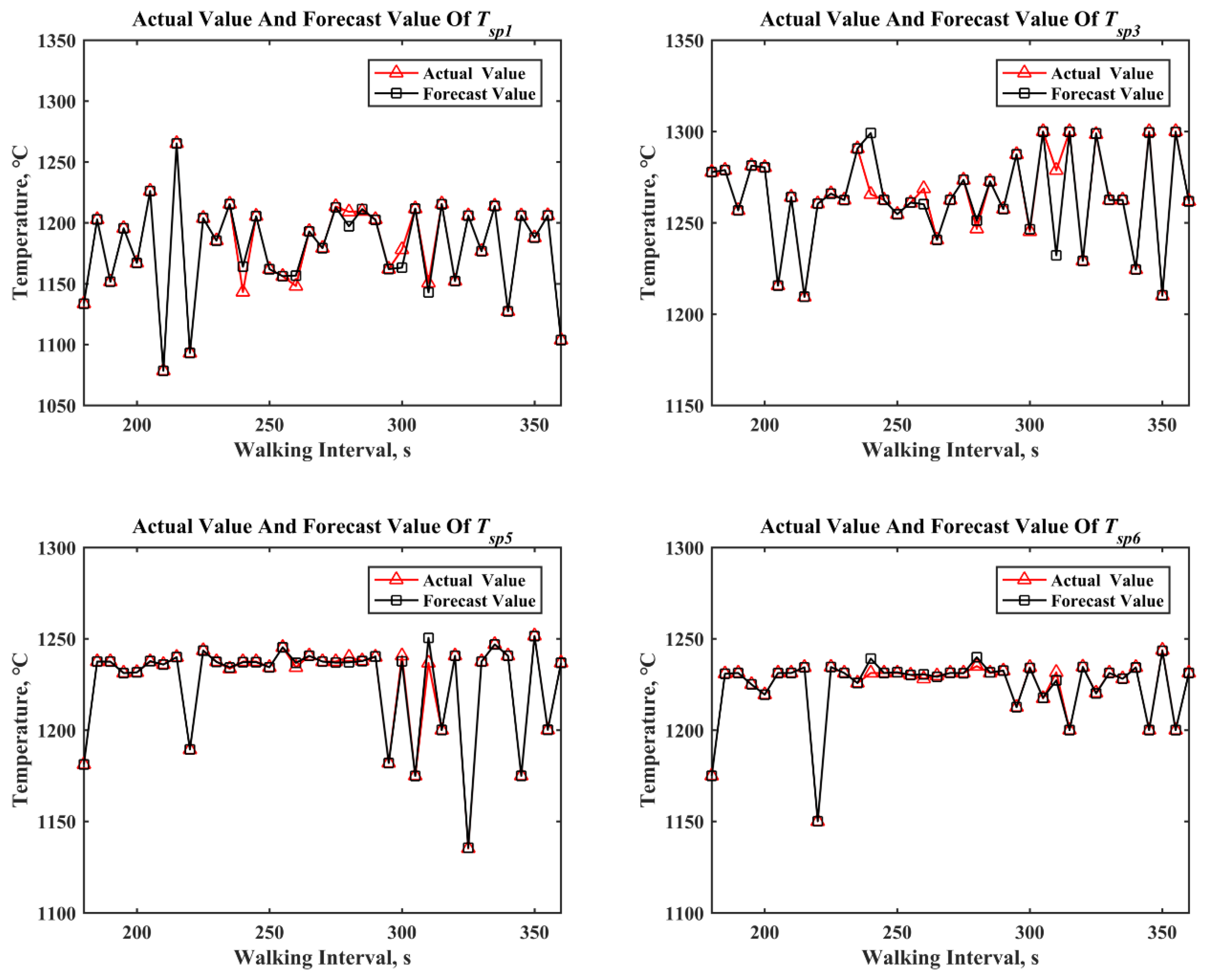
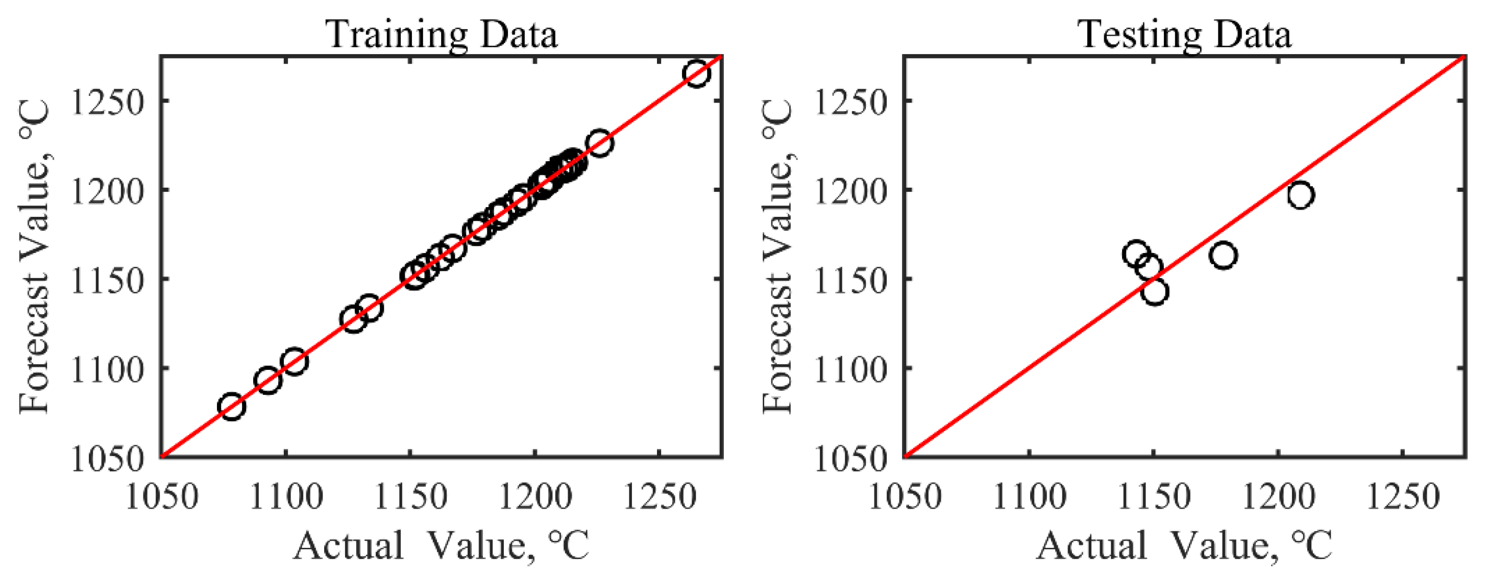
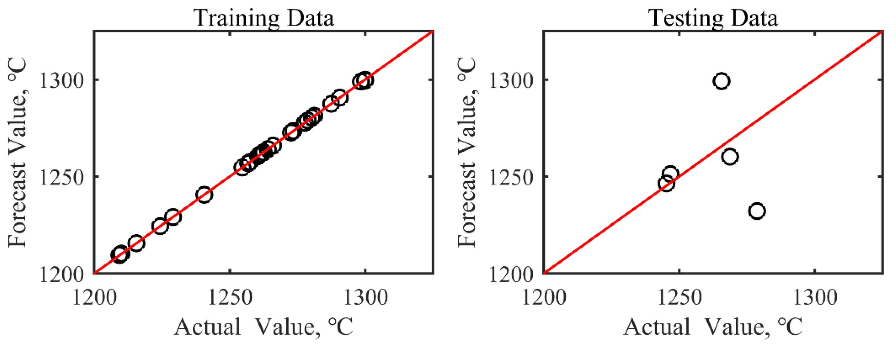
J ( T s p   ) = T s p 1 × 1 T s p 1 × T s p 3 × 1 T s p 3 × T s p 5 × 1 T s p 5 × T s p 6 × 1 T s p 6 × i = 1 n Δ T i d i s 2 + M i = 1 n Δ T i m a x 2 + N i = 1 n S F C i 2 ( T s p 1 0 , T s p 3 0 , T s p 5 0 , T s p 6 0 )
where Tsp1, Tsp3, Tsp5 and Tsp6 are the set-point temperatures of control zone 1, 3, 5 and 6 respectively.
While being equivalent to Equation (1), Equation (3) has the advantage that it can be minimized by HJDSA by setting set-point temperature values near their initial values; hence why Equation (3) can be regarded as a set-point temperatures generator. This generator and the zone model are two separate units, written in FORTRAN for this paper, which pass parameters to each other. Figure 4 illustrates the overall program flow chart of HJDSA for determining the desired set-point temperatures.
Parameters should be set first. Initial set-point temperatures Tsp1, Tsp3, Tsp5 and Tsp6 were chosen to be 1150 °C, 1250 °C, 1200 °C and 1200 °C respectively, and an initial increment of 25 was used for all variables. In order to terminate the algorithm, the termination value εs and step length s were introduced which set to 1.0 × 10⁻⁶ and 25, respectively. The final parameter is ρ (ρ = 0.5) which was used to reduce increments εi (i = 1, ..., 4, for the 4 different variables) and step length at each iteration. After reading initial set-point temperatures as base point, an exploratory move begins. If the exploratory move and a pattern move following this both succeed, the increments and step length will reduce, and the next iteration commences. The iteration continues until the step length is less than the termination value.

2.3. Neural Network

It takes almost 5 h, using a desktop computer with two Inter Xeon E5–2670 processors and 16 GB RAM, for each scenario to obtain the desired set-point temperatures by HJDSA. It is inevitable that the production rate will change during an actual industrial process, and the delay of a further to determine the next group of desired set-point temperatures is impractical. This is a limitation of the zone model approach, making it incapable of real time prediction [6]. To overcome this limitation, four back propagation neural networks will be used for the determination of the four desired set-point temperatures. The neural networks are trained based on the precise data calculated by HJDSA with different production rates. Since there is a small increment between the production rates, the neural networks not only have sufficient precise training data, but can also mimic the optimisation process performed by HJDSA, thus making it run faster.

2.3.1. Data Processing

To obtain a sufficient quantity of accurate input data for the neural networks, the HJDSA, for which heating accuracy (ΔTdis) was given priority and which also emphasized the importance of heating uniformity (ΔTmax) (i.e., scenarios I and IV in Table 1), was used to obtain desired set-point temperatures. The temperatures were determined every 1.75 ton/h increment from the minimum production rate (65 ton/h) to the maximum production rate (130 ton/h). Since the production rate grows in inverse proportion to walking interval, the main program increased walking interval with an increment value of 5s from 180s to 360s to obtain different production rates. Therefore, there were 37 different set-point temperatures with different walking interval, ΔTdis and ΔTmax. Of these, 10 sets of the data are illustrated in Table 2 as example.
To eliminate the deviation derived from different input values, using arithmetic mean method is necessary to normalise the data. The mean value can be calculated using Equation (4) [28]:
x = 2 × x 0 x m i n x m a x x m i n 1 ,
where x0 is defined as an initial data value among the input data groups, and xmin and xmax express the minimum and maximum values among the input data groups, respectively.

2.3.2. Parameters for Back Propagation (BP) Neural Network

A three-layer BP neural network [26] is used to construct the model for the optimisation of set-point temperatures (Figure 5). The activation function of hidden layer and output layer are both chosen to be the tan-sigmoid transfer function, tansig, the expected mean squared error is taken as 0.0001, and the learning rate is 0.1. After comparing the performance different training algorithms including Levenberg-Marquardt, Bayesian Regularization, Scaled Conjugate Gradient and Resilient, this paper chose Levenberg-Marquardt as training algorithm for best forecasting results. The input layer has three neurons: WI is walking interval, ΔTdis is heating accuracy, and ΔTmax is heating uniformity. There is one hidden layer, which contains 8 neurons. Since there are a small group of training data (32 sets), it is hard to build a complex neural network to reflect the relationship between inputs and outputs. Suppose that construct a 3X4 neural network with 3 above inputs, and 4 outputs for 4 set-point temperatures, it needs more than 15 neurons in hidden layer to reach the expected mean squared error. However, when tested the trained network, the overfitting occurred. Therefore, this study set one neuron in the output layer, and four BP neural networks are then constructed for four set-point temperatures (Tsp1, Tsp3, Tsp5 and Tsp6) respectively. In order to obtain the desired results, 5 sets of input data were selected for testing and the rest for training.
After training the BP neural network learning algorithm on the samples, the neural network can reflect the relationship between the three important input parameters and the set-point temperatures. Through proper adjustment of the walking interval, heating accuracy and heating uniformity, the appropriate set-point temperatures are determined. Using the well-trained BP neural network, the main program can calculate desired set-point temperatures immediately, meaning effectively that the zone model is made capable of real time prediction.

3. Results

The described optimisation method was able to achieve accurate control of temperature for discharge blooms with the heating accuracy within 1 °C in all scenarios. Furthermore, the neural networks, trained with precise data calculated by HJDSA, could mimic the optimisation process of HJDSA, thus making it run faster.

3.1. The Proposed Optimisation Method

It took almost 5 h for each case to reach the desired set-point temperatures by HJDSA. Although weighted factors in Equation (4) were used to ensure that the changes of ΔTdis, ΔTmax, and SFC are at same level, the set-point temperatures of scenarios I and III are the same (Table 3). This is because ΔTmax fluctuates more than SFC, since SFC is an average quantity which not only depends on set-point temperatures but also on furnace running time, and because the rate of change of ΔTmax was about five times larger than that of SFC. Thus, ΔTmax dominates.
In this study, all optimisation strategies (ΔTdis, together with ΔTmax and/or SFC) greatly improve the heating accuracy within 1 °C (ΔTdis in Table 4). When the objective of specific fuel consumption is emphasized without including ΔTmax in the optimisation, as in scenarios II and V, poorer heating uniformity resulted (ΔTmax shown in Table 4), especially for scenario II, which was worst among all scenarios. Furthermore, the set-point temperature of control zone 1 (preheating zone) of this scenario was lowest under production rate of 130 tonnes per hour which means that less fuel is input for less fuel consumption. In order to maintain the heating accuracy, the burner in soaking zone (control zone 5 and control zone 6) would have a higher fire rate, which results in higher set-point temperatures (Tsp5 and Tsp6 in Table 3). Therefore, a very large set-point temperature difference between preheating zone and soaking zone (about 120 °C) resulted, and heating uniformity was poorest.

3.2. Neural Network

The four BP neural networks were trained in MATLAB (Version 2016b, MathWorks, Natick, MA, USA) using neural network toolbox, and after meeting the expected mean squared error the training process terminated, and biases and weights were output to be used in main program written in FORTRAN. When training the neural networks, in most of the tests, it takes few seconds to meet the expected mean squared error. After 468 training epochs, the network used for predicting Tsp1, achieved the expected mean squared error and got best forecasting performance; 193 training epochs were needed for Tsp3, 363 training epochs for Tsp5 and 305 training epochs for Tsp6. The well-trained neural networks should not need to be retrained, since the training data collected by the changes of walking interval from 180 s to 360 s to obtain different production rates with a small increment value of 5 s, when inputting a new walking interval not including in the training data to the networks, it is hard to disobey the rules of input-output relationship in the networks. Which makes the predicted set-point temperatures appropriate enough. In addition, the real valve of ΔTdis calculated by can be within ±5 °C, through manual adjustment of input parameters of the networks to fine tuning the output set-point temperatures, and the input values of ΔTmax for different range groups of walking interval can be seen in Table 5.
Once the expected mean squared error is obtained through network training, the forecast values of set-point temperatures for the four control zones are determined and compared with actual values (the 37 sets of temperature data calculated by HJDSA) to evaluate the forecast results. Figure 6 shows the well-trained networks which compare the forecast values with the actual values. As for the prediction performance, the results of the training samples and testing ones are shown in Figure 7, Figure 8, Figure 9 and Figure 10, with different neural networks, illustrating that the predicted values trace well the practical data.
The four well-trained networks can be written as Equation (5), and the main program calls them to calculate set-point temperatures when the walking interval changes. In this equation, WI is walking interval, which is between 180 and 360, and the value of ΔTdis is zero for best heating accuracy. The value of ΔTmax, depends on the real value of ΔTdis calculated by the program. By manual adjustment, the real valve of ΔTdis can be within ±5 °C, and the values of ΔTmax for different range groups of walking interval can be seen in Table 5. Notice that the value of ΔTmax from 220 s to 235 s is higher than 10, because the actual value of ΔTmax on 235 s calculated by HJDSA is 13 and the value of ΔTmax is selected nearby the boundary to ensure desired heating accuracy.
{ f ( W I , Δ T d i s   , Δ T m a x ) n e t 1 = T s p 1 f ( W I , Δ T d i s , Δ T m a x ) n e t 2 = T s p 3 f ( W I , Δ T d i s , Δ T m a x ) n e t 3 = T s p 5 f ( W I , Δ T d i s , Δ T m a x ) n e t 4 = T s p 6
Figure 11 shows drop-out temperature of slabs with different walking intervals. The furnace started with the trial condition in Table 3, and altered to the set-point temperatures calculated by HJDSA with walking interval of 180 s at time 0. After drop-out temperature stabilised, the program altered the walking interval to another value at 6120 time point and the set-point temperatures changed at same time. The new set-point temperatures were calculated by BP neural networks. The furnace model which used set-point temperatures calculated by HJDSA had better heating accuracy with a value of ΔTdis within ±1 °C, comparing to ±5 °C by BP neural networks. It can also be seen that the drop-out temperature has a sharp increase or decrease when the waking interval is increased, when the walking interval and the set-point temperatures changed at same time, some slabs in the soaking zone with the new walking interval were either overheated or could not soak enough heat.
Considering now the computing time of the two methods, the computational efficiency of the BP neural network is fairly promising, taking a few milliseconds, comparing to 5 h with HJDSA. This implies that real time simulation of zone model is successfully maintained when production rate changes.

4. Discussion

Comparing to the method which solve PDE optimal control problem to get set-point temperatures [18], both of results can highly improve heating accuracy, with an average deviation of less than 1 °C from the target discharge temperature, and the method solved PDE problem have a promising computational efficiency which spent a few seconds to get optimisation set-point temperatures. However, the method is tailored to an atypical control system which may be invalid for other furnaces. The method of this paper has the benefit that this optimisation strategy is a common method and is therefore suitable for any other furnaces. Hence the proposed method of this paper has much more potential for broad application.
When making a comparison between HJDSA and GA, it is obvious that HJDSA performs better in multi-objective optimisation problems. Not only does using HJDSA obtain a better heating accuracy, but it also avoids local optimisation. Considering the optimal results of [19] about scenarios I and IV in Table 3, it can be seen that the two Tsp1 are same in these scenarios and the two Tsp5 are also the same. Moreover, there is little difference between the other two optimal temperatures respectively —no more than 10 °C. These abnormally similar results of the two scenarios with different production rates implies that the GA may have a local optimum of the objective function. Further support for this conclusion is that the ΔTdis and ΔTmax in Table 4 are nearly the same for the two scenarios.
Furthermore, comparing the optimised heating curves for the different scenarios in Figure 12, it can be seen clearly in that both of the results can achieve improved heating accuracy, and regardless of whether temperature uniformity or specific fuel consumption is emphasised, the temperature of a certain bloom in a specific position in this paper is lower, which turns out the results of this paper demonstrate less energy consumption. To be more specific, from the detailed data in Table 6, it can be seen that it saves more than 2.5 MW—regardless of whether it is scenario I or II.
Overall, the proposed method of this paper is a common method which is thus suitable for any other furnaces, it has much more potential for broad application. These results show that the proposed method can highly improve heating accuracy, less than 1 °C from the target discharge temperature. However, the computing time of each scenario is too long for real time simulation when production rate changes. Therefore, a further optimisation based on BP neural network was used to calculate the set-point temperatures immediately when production rate changes, and the results show the furnace model which used set-point temperatures calculated by BP neural network had a sharp increase or decrease of the drop-out temperature when the waking interval is increased, which might be a direction of future work, i.e., focus on erase the fluctuation of the drop-out temperature as the waking interval changes.

5. Conclusions

This paper presents a function-value based multi-objective optimisation of reheating furnace operations, and highlights a novel method with HJDSA based on zone model. A set of optimisation scenarios was defined, taking into account the difference between the desired and the real discharge temperature, the maximum temperature difference in bloom cross section and also specific fuel consumption. The results show that the proposed method can highly improve heating accuracy, while a balance is kept between the optimisation objectives of temperature uniformity and specific fuel consumption. Comparing with the optimisation method based on GA, the proposed method could not only avoid local optimisation, but also exhibited lower energy consumption. However, the computing time of each scenario of approximately five hours is too long for real time simulation when production rate changes. Therefore, a further optimisation was introduced which was based on the data calculated by HJDSA, and used BP neural network to calculate the set-point temperatures. The results show the average deviation less than 5 °C, from the desired discharge temperature which is excellent, and the BP neural network was able to calculate the set-point temperatures immediately, meeting the requirements for real time simulation.

Author Contributions

B.G. have contributed to developing ideas about the optimisation of furnace operations by HJDSA, building, training and testing the neural networks and finishing the writing of this paper. C.W., C.K.T., P.A.R. and L.V. reviewed the paper and provided valuable opinions during the manuscript writing. Y.H. helped with the structuring, writing the paper and analysing the results. All authors read and approved the final manuscript for submission.

Funding

This research was funded by The National Natural Science Foundation of China (Grant No. 61573381), Fundamental Research Funds for the Center Universities of Center South University (Grant No. 2017zzts692) and Engineering and Physical Sciences Research Council (Grant No. EP/P004636/1, UK).

Conflicts of Interest

The authors declare no conflict of interest.

Nomenclature

SymbolsDefinitionUnit
u(t)firing rate at the current time-step-
y(t)the required temperature compensation relative to the set-point temperature at the current time-step°C
ΔTdisthe difference between the desired and the realized discharge temperature, which represents heating accuracy°C
ΔTmaxthe maximum temperature difference in bloom cross section, which represents heating uniformity°C
SFCspecific fuel consumptionGJ tonne−1
Mweighted factor of ΔTmax-
Nweighted factor of SFC-
Tspset-point temperature°C
Tsp1set-point temperature of control zone 1°C
Tsp3set-point temperature of control zone 3°C
Tsp5set-point temperature of control zone 5°C
Tsp6set-point temperature of control zone 6°C
WIwalking intervals
abase point-
bpattern point-
xvariable-
εincrement-
sstep length-
εsterminate value-
ρreduction value-

References

  1. International Energy Agency (IEA). World Energy Outlook 2013. Available online: https://www.iea.org/publications/freepublications/publication/WEO2013.pdf (accessed on 1 October 2017).
  2. International Energy Agency. Renewables Information 2012. IEA Stat. 2012, 497. [Google Scholar] [CrossRef]
  3. McBrien, M.; Serrenho, A.C.; Allwood, J.M. Potential for energy savings by heat recovery in an integrated steel supply chain. Appl. Therm. Eng. 2016, 103, 592–606. [Google Scholar] [CrossRef]
  4. Singh, V.K.; Talukdar, P. Comparisons of different heat transfer models of a walking beam type reheat furnace. Int. Commun. Heat Mass Transf. 2013, 47, 20–26. [Google Scholar] [CrossRef]
  5. Environmental Protection Agency (EPA, U.S.). Available and Emerging Technologies for Reducing Greenhouse Gas Emissions from the Iron and Steel Industry 2012. Available online: https://www.epa.gov/sites/production/files/2015-12/documents/ironsteel.pdf (accessed on 14 October 2017).
  6. Hu, Y.; Tan, C.K.; Broughton, J.; Roach, P.A. Development of a first-principles hybrid model for large-scale reheating furnaces. Appl. Energy 2016, 173, 555–566. [Google Scholar] [CrossRef]
  7. Hu, Y.; Yan, J. Numerical simulation of radiation intensity of oxy-coal combustion with flue gas recirculation. Int. J. Greenh. Gas Control 2013, 17, 473–480. [Google Scholar] [CrossRef]
  8. Hu, Y.; Li, H.; Yan, J. Numerical investigation of heat transfer characteristics in utility boilers of oxy-coal combustion. Appl. Energy 2014, 130, 543–551. [Google Scholar] [CrossRef]
  9. Hu, Y.; Niska, J.; Broughton, J.; McGee, E.; Tan, C.K.; Matthew, A.; Roach, P. Zone modelling coupled with dynamic flow pattern for the prediction of transient performance of metal reheating. AISTech Iron Steel Technol. Conf. Proc. 2014, 3, 3395–3408. [Google Scholar]
  10. Basso, D.; Cravero, C.; Reverberi, A.P.; Fabiano, B. CFD analysis of regenerative chambers for energy efficiency improvement in glass production plants. Energies 2015, 8, 8945–8961. [Google Scholar] [CrossRef]
  11. Al-Abbas, A.H.; Naser, J.; Dodds, D. CFD modelling of air-fired and oxy-fuel combustion of lignite in a 100KW furnace. Fuel 2011, 90, 1778–1795. [Google Scholar] [CrossRef]
  12. Casal, J.M.; Porteiro, J.; Míguez, J.L.; Vázquez, A. New methodology for CFD three-dimensional simulation of a walking beam type reheating furnace in steady state. Appl. Therm. Eng. 2015, 86, 69–80. [Google Scholar] [CrossRef]
  13. Prieler, R.; Mayr, B.; Demuth, M.; Holleis, B.; Hochenauer, C. Prediction of the heating characteristic of billets in a walking hearth type reheating furnace using CFD. Int. J. Heat Mass Transf. 2016, 92, 675–688. [Google Scholar] [CrossRef]
  14. Filipponi, M.; Rossi, F.; Presciutti, A.; De Ciantis, S.; Castellani, B.; Carpinelli, A. Thermal analysis of an industrial furnace. Energies 2016, 9, 833. [Google Scholar] [CrossRef]
  15. Hottel, H.C.; Cohen, E.S. Radiant exchange in a gas-fired enclosure: allowance for nonuniformity of gas temperature. AIChE J. 1958, 4, 3–14. [Google Scholar] [CrossRef]
  16. Zhou, W.; Qiu, T. Zone modeling of radiative heat transfer in industrial furnaces using adjusted Monte-Carlo integral method for direct exchange area calculation. Appl. Therm. Eng. 2015, 81, 161–167. [Google Scholar] [CrossRef]
  17. Tan, C.K.; Jenkins, J.; Ward, J.; Broughton, J.; Heeley, A. Zone modelling of the thermal performances of a large-scale bloom reheating furnace. Appl. Therm. Eng. 2013, 50, 1111–1118. [Google Scholar] [CrossRef]
  18. Yang, Z.; Luo, X. Optimal set values of zone modeling in the simulation of a walking beam type reheating furnace on the steady-state operating regime. Appl. Therm. Eng. 2016, 101, 191–201. [Google Scholar] [CrossRef]
  19. Hu, Y.; Tan, C.K.; Broughton, J.; Roach, P.A.; Varga, L. Model-based multi-objective optimisation of reheating furnace operations using genetic algorithm. Energy Procedia 2017, 142, 2143–2151. [Google Scholar] [CrossRef]
  20. Rocha, M.; Neves, J. Preventing Premature Convergence to Local Optima in Genetic Algorithms via Random Offspring Generation. Lect. Notes Comput. Sci. 1999, 1611, 127–136. [Google Scholar] [CrossRef] [Green Version]
  21. Hooke, R.; Jeeves, T.A. “Direct Search” Solution of Numerical and Statistical Problems. J. ACM 1961, 8, 212–229. [Google Scholar] [CrossRef]
  22. Rostek, K.; Morytko, Ł.; Jankowska, A. Early detection and prediction of leaks in fluidized-bed boilers using artificial neural networks. Energy 2015, 89, 914–923. [Google Scholar] [CrossRef]
  23. Tan, C.K.; Wilcox, S.J.; Ward, J. Use of artificial intelligence techniques for optimisation of co-combustion of coal with biomass. J. Energy Inst. 2006, 79, 19–25. [Google Scholar] [CrossRef]
  24. (PDF) On-Line Slab Temperature Calculation and -Control. Available online: https://www.researchgate.net/publication/236888905_ONLINE_SLAB_TEMPERATURE_CALCULATION_AND_-CONTROL (accessed on 16 October 2017).
  25. Chen, S.H.; Jakeman, A.J.; Norton, J.P. Artificial Intelligence techniques: An introduction to their use for modelling environmental systems. Math. Comput. Simul. 2008, 78, 379–400. [Google Scholar] [CrossRef]
  26. Rumelhart, D.E.; Hinton, G.E.; Williams, R.J. Learning representations by back-propagating errors. Nature 1986, 323, 533–536. [Google Scholar] [CrossRef]
  27. Kirgat, G.S.; Surde, A.N. Review of Hooke and Jeeves Direct Search Solution Method Analysis Applicable to Mechanical Design Engineering. Int. J. Innov. Eng. Res. Technol. 2014, 1, 1–14. [Google Scholar]
  28. Patro, S.G.K.; Sahu, K.K. Normalization: A Preprocessing Stage. [1503.06462] Normalization: A Preprocessing Stage. Available online: https://arxiv.org/abs/1503.06462 (accessed on 2 July 2017).
Figure 1. The steps of proposed method in this paper.
Energies 11 02324 g001
Figure 2. Outline of the reheating furnace.
Energies 11 02324 g002
Figure 3. Level-2 module-based process control solution.
Energies 11 02324 g003
Figure 4. Flow chart of Hooke-Jeeves direct search algorithm (HJDSA) for seeking desired set-point temperatures.
Energies 11 02324 g004
Figure 5. Back propagation (BP) neural network prediction models.
Energies 11 02324 g005
Figure 6. Actual value and forecast value of set-point temperatures.
Energies 11 02324 g006
Figure 7. Actual value and forecast value of Tsp1.
Energies 11 02324 g007
Figure 8. Actual value and forecast value of Tsp3.
Energies 11 02324 g008
Figure 9. Actual value and forecast value of Tsp5.
Energies 11 02324 g009
Figure 10. Actual value and forecast value of Tsp6.
Energies 11 02324 g010
Figure 11. Comparison of drop-out temperature of slab with different walking intervals. WI: walking interval.
Energies 11 02324 g011
Figure 12. Comparison of heating curves under different optimisation scenarios and methods.
Energies 11 02324 g012
Table 1. Specification of different optimisation scenarios and weighted factors.
ScenarioProduction Rate, ton/hOptimisation Objectives 1MN
I130ΔTdisΔTmax/10
II130ΔTdis/SFC010
III130ΔTdisΔTmaxSFC110
IV65ΔTdisΔTmax/10
V65ΔTdis/SFC010
VI65ΔTdisΔTmaxSFC110
1ΔTdis, the difference between the desired and the realistic discharge temperature (°C), which represents heating accuracy; ΔTmax, the maximum temperature difference in the slab cross section (°C), which represents heating uniformity; the specific fuel consumption (SFC; GJ/t).
Table 2. Heating performance and optimal furnace set-point temperatures of different optimisation scenarios.
Production Rate, ton/hWalking Interval, sΔTdis, °CΔTmax, °CTsp1, °CTsp3, °CTsp5, °CTsp6, °C
653600.1984.0001103.61261.81236.81231.3
723400.2326.0001127.31224.41240.61234.4
793200.1424.0971152.21229.21240.61234.6
863000.3394.0091178.11245.31240.61234.4
932800.5064.0001209.01246.71240.01235.0
1002600.3394.2101148.11268.81234.41228.1
1072400.7194.0001143.21265.61237.51231.2
1142200.3378.0001093.01260.51189.41150.0
1212000.0144.0001167.01280.31231.61219.4
1301800.2945.2681133.61277.71181.31175.0
Table 3. Optimal furnace set-point temperatures of different optimisation scenarios.
ScenarioTsp1, °CTsp3, °CTsp5, °CTsp6, °C
Trial1200130012501250
I1134127811811175
II1088127312011227
III1134127811811175
IV1104126212371231
V1061126912341222
VI1104126212371231
Table 4. Heating performance of different optimisation scenarios.
ScenarioΔTdis, °CΔTmax, °CSFC, GJ/tonne
Trial3591.50
I<151.369
II<1121.299
III<151.369
IV<141.730
V<181.575
VI<141.730
Table 5. Values of ΔTmax for walking interval between 180 and 360.
Range of Walking Interval, s180–220220–235235–240240–250250–360
Value of ΔTmax, °C512.5254
Table 6. Comparison of energy input under different optimisation scenarios and methods.
ScenarioTrialData from [19]This Paper
IIIIII
Energy input, MW54.452.750.849.947.8

