Incremental Capacity Analysis on Commercial Lithium-Ion Batteries using Support Vector Regression: A Parametric Study


 ,
,  ,
,
Abstract
1. Introduction
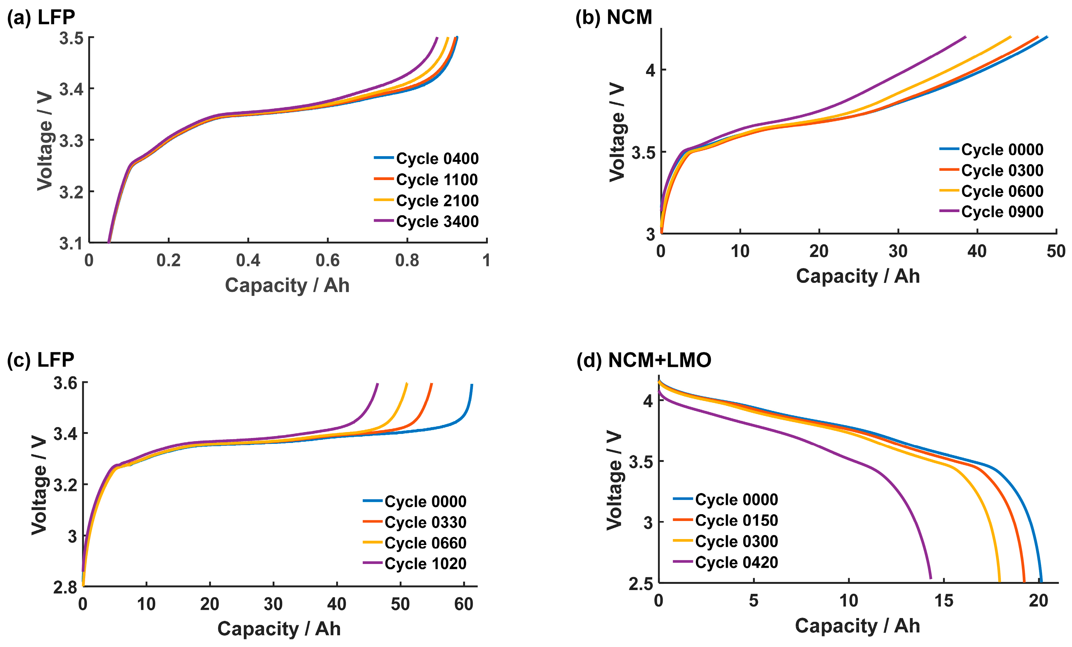
2. Experimental
3. Methodology
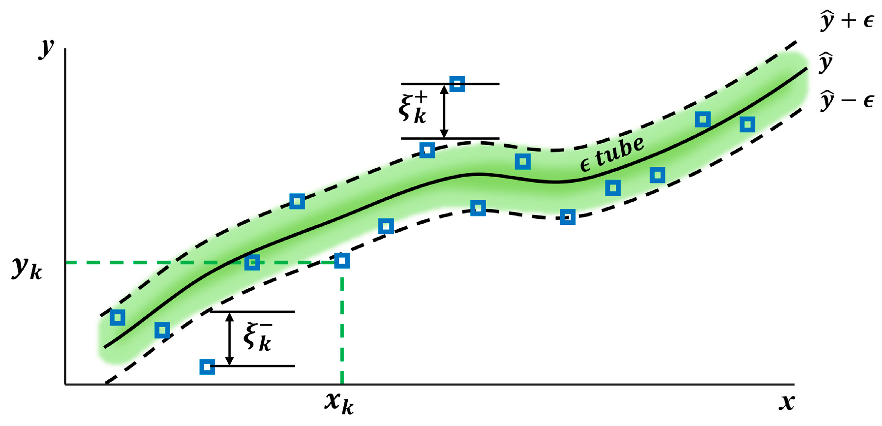
3.1. The Canonical Form of the Support Vector Regression
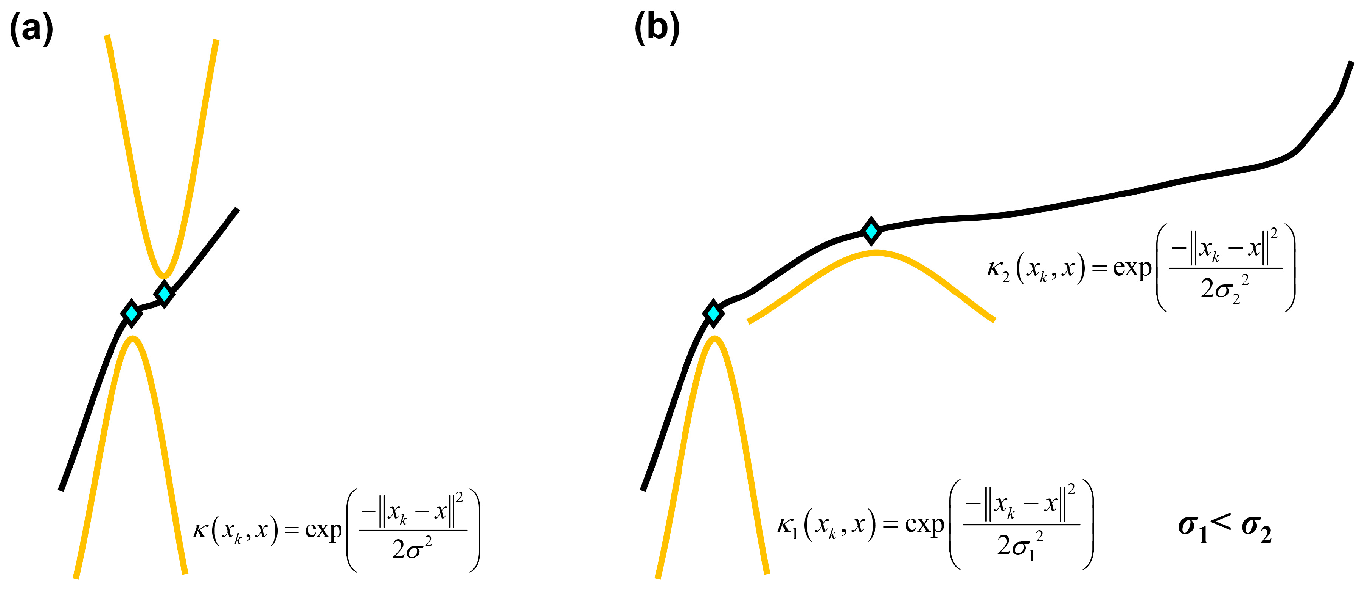
3.2. Double σ to Enhance the Quality of Curve Fitting
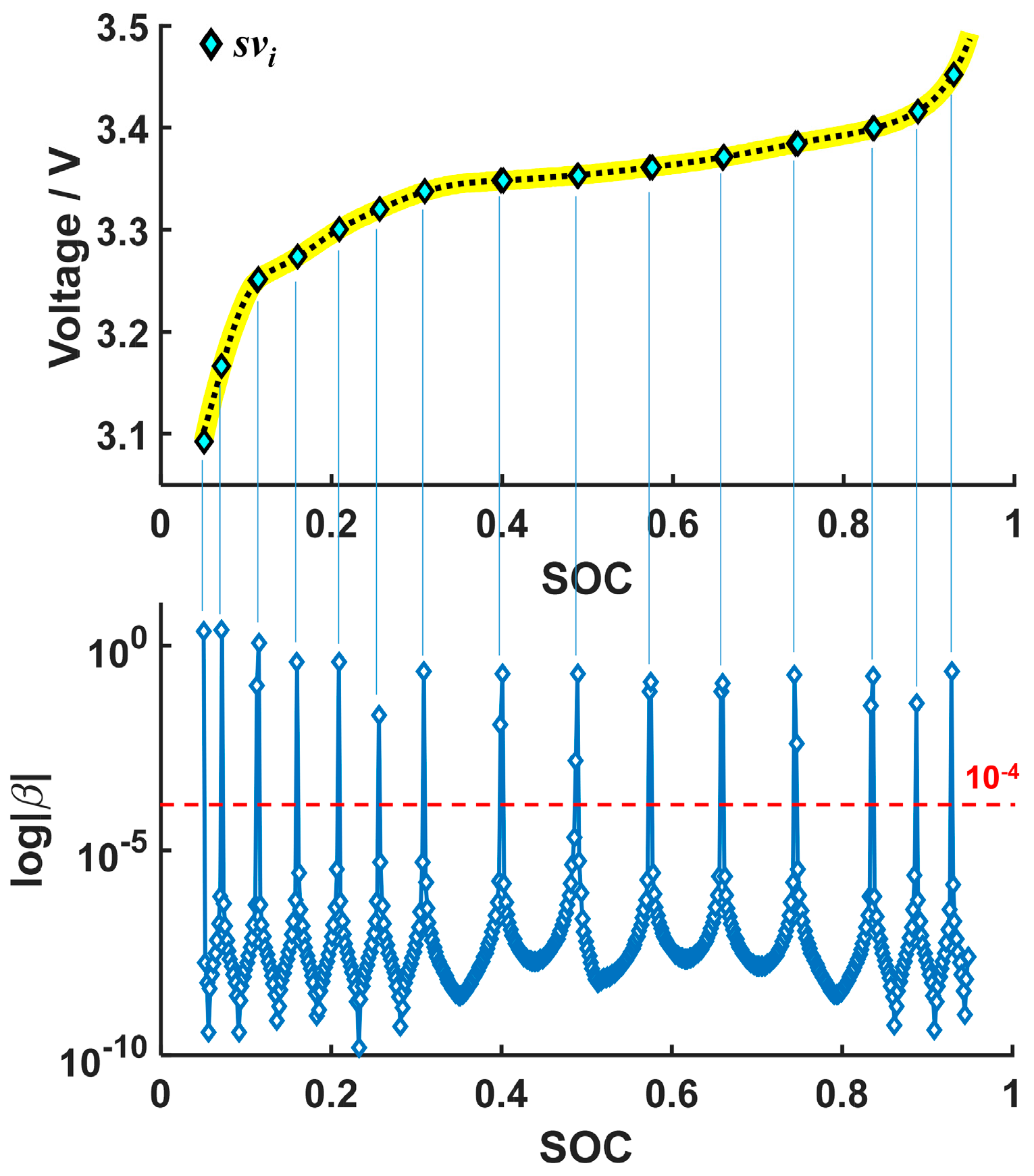
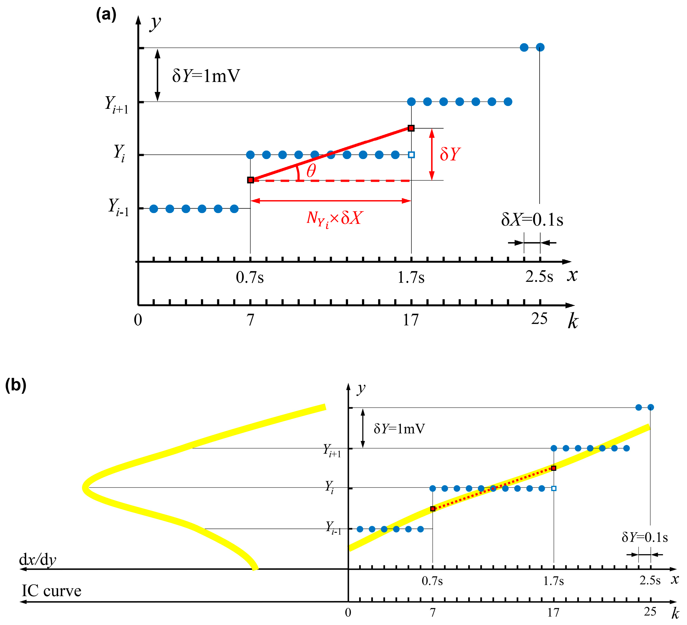
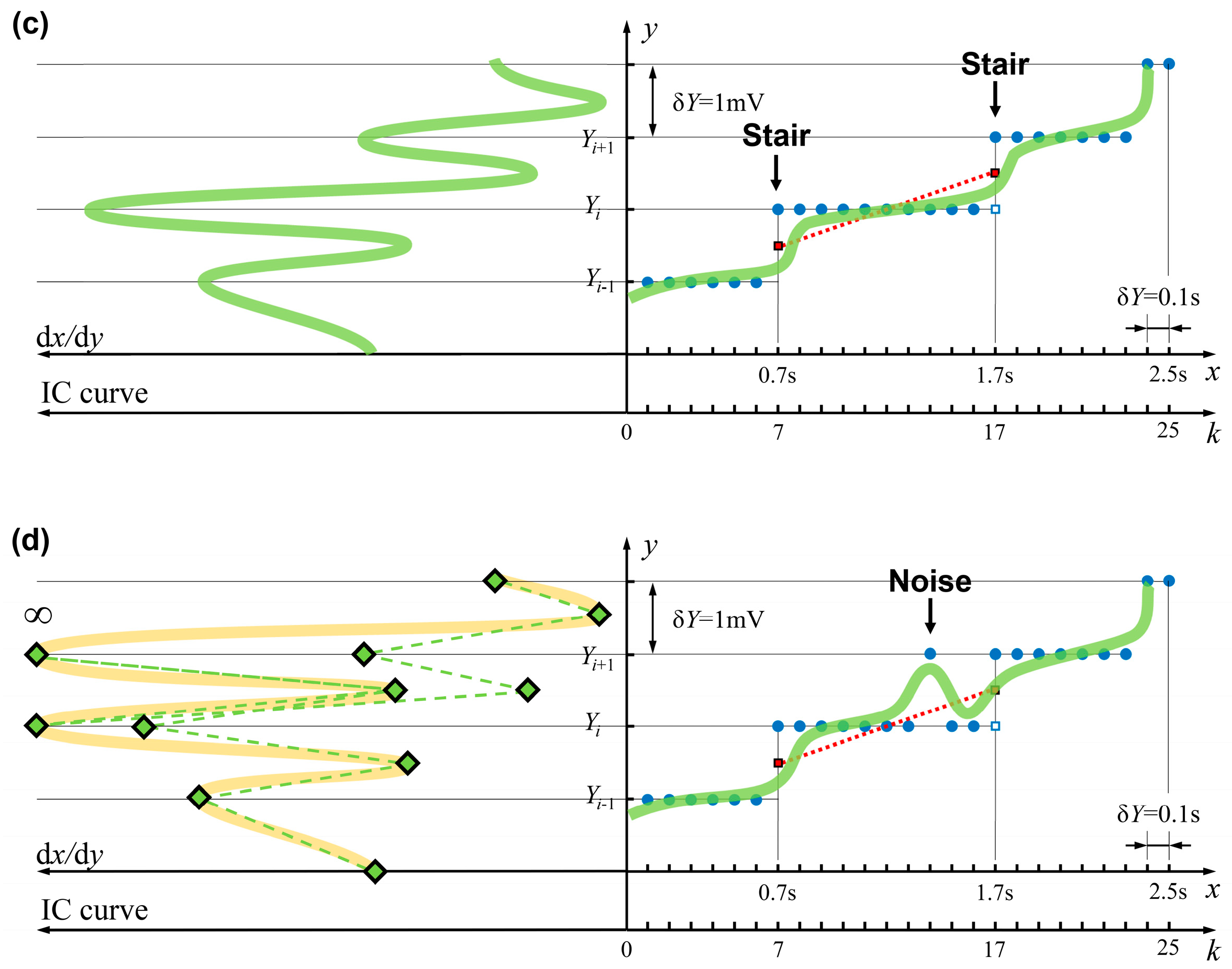
3.3. Criterion for Evaluating the Quality of Curve Fitting by SVR
3.4. Changing the Cost Functions to Improve the Accuracy of Incremental Capacity Analysis
4. Result and Discussions
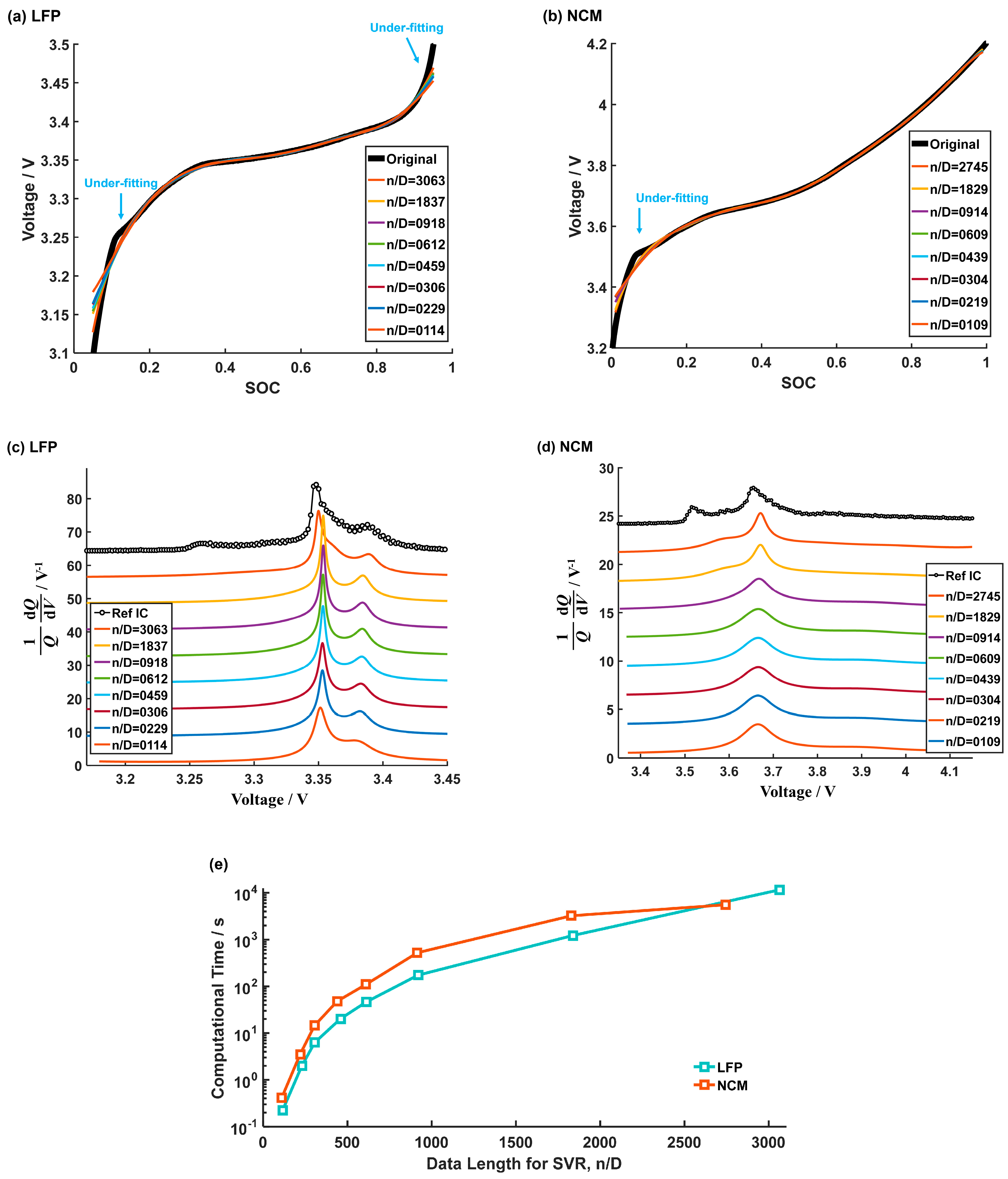
4.1. The Influence of the Data Length on the Performances of the SVR Algorithm
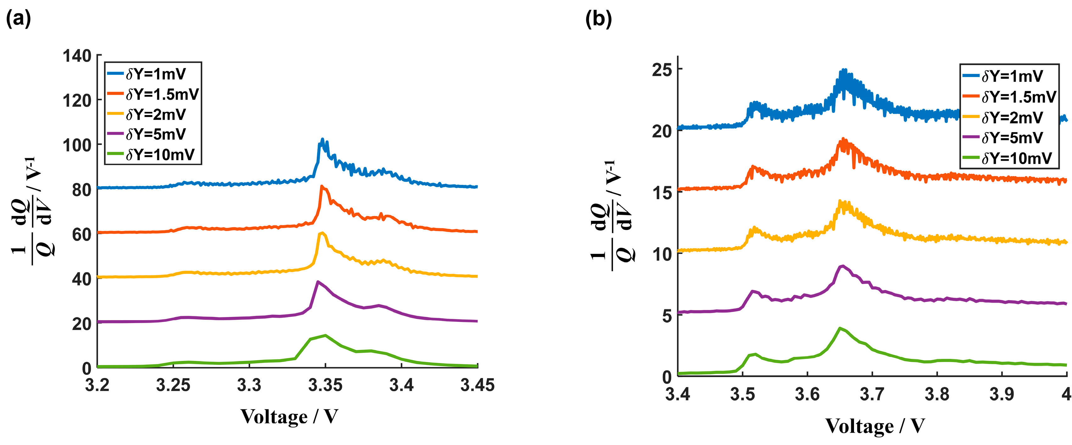
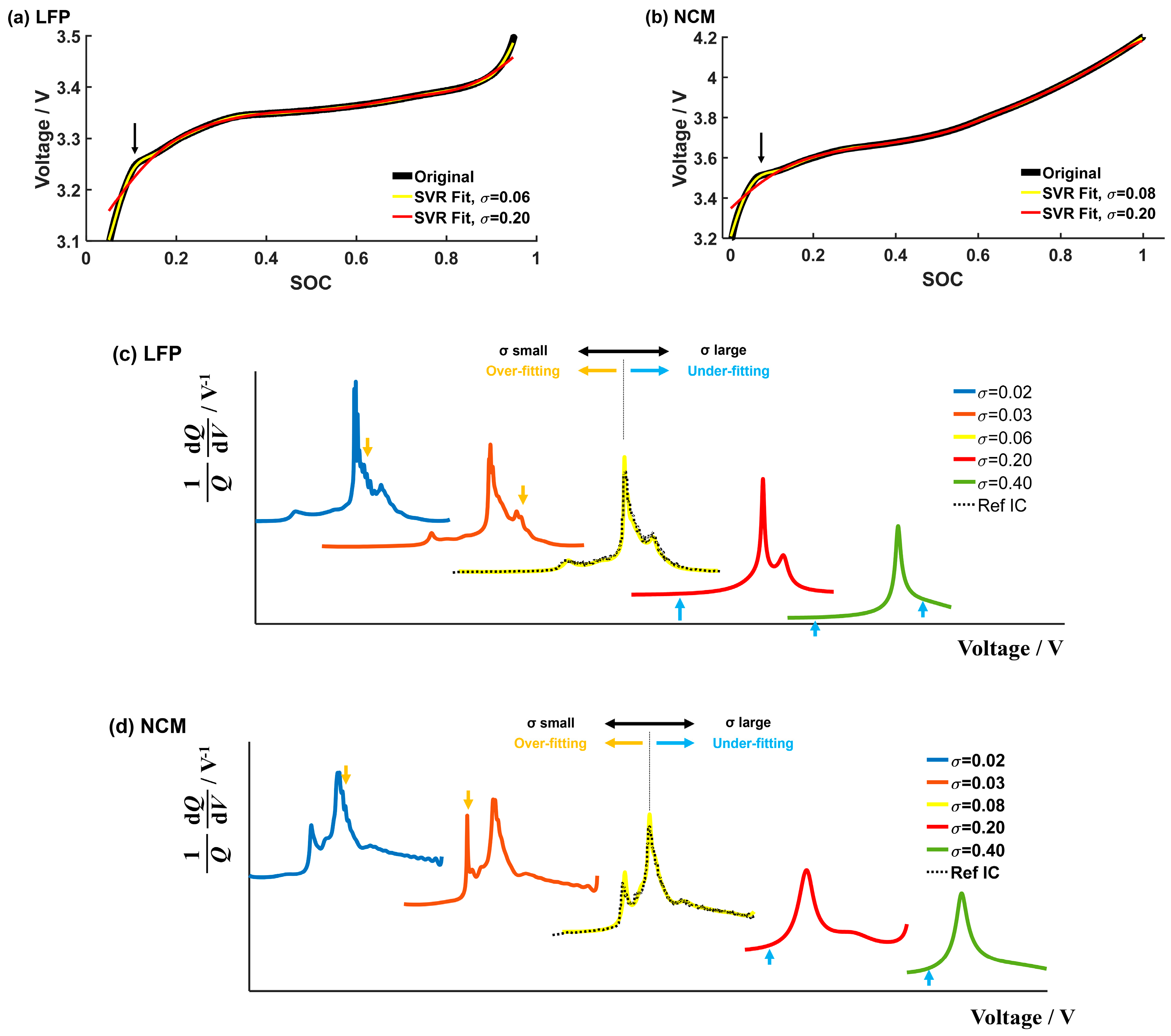
4.2. The Influence of the σ in the Gaussian Kernel on the Performance of the SVR Algorithm
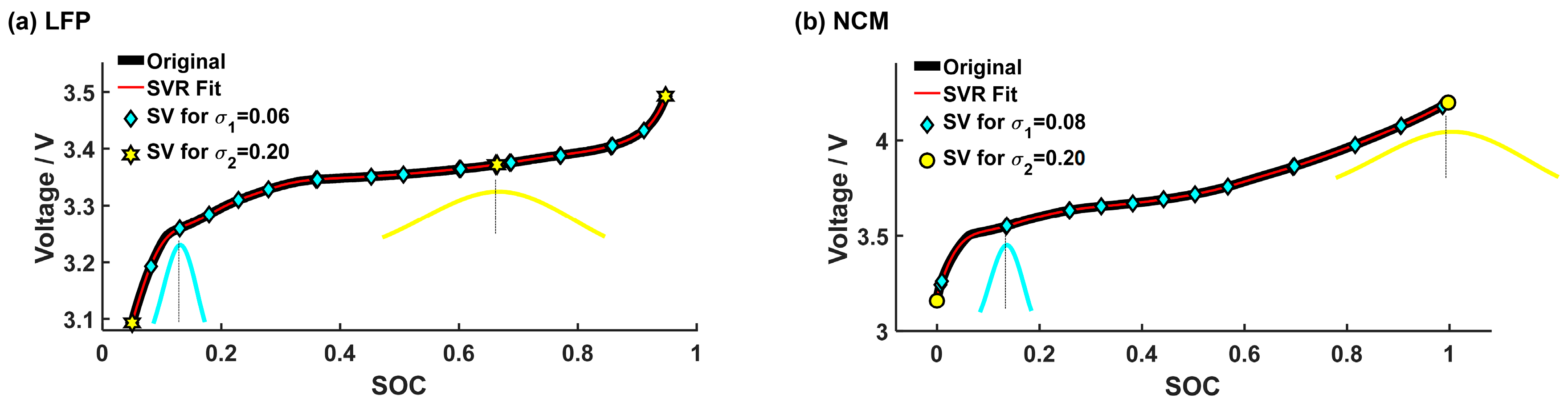
4.3. Double σ to Enhance the Accuracy of the SVR Algorithm
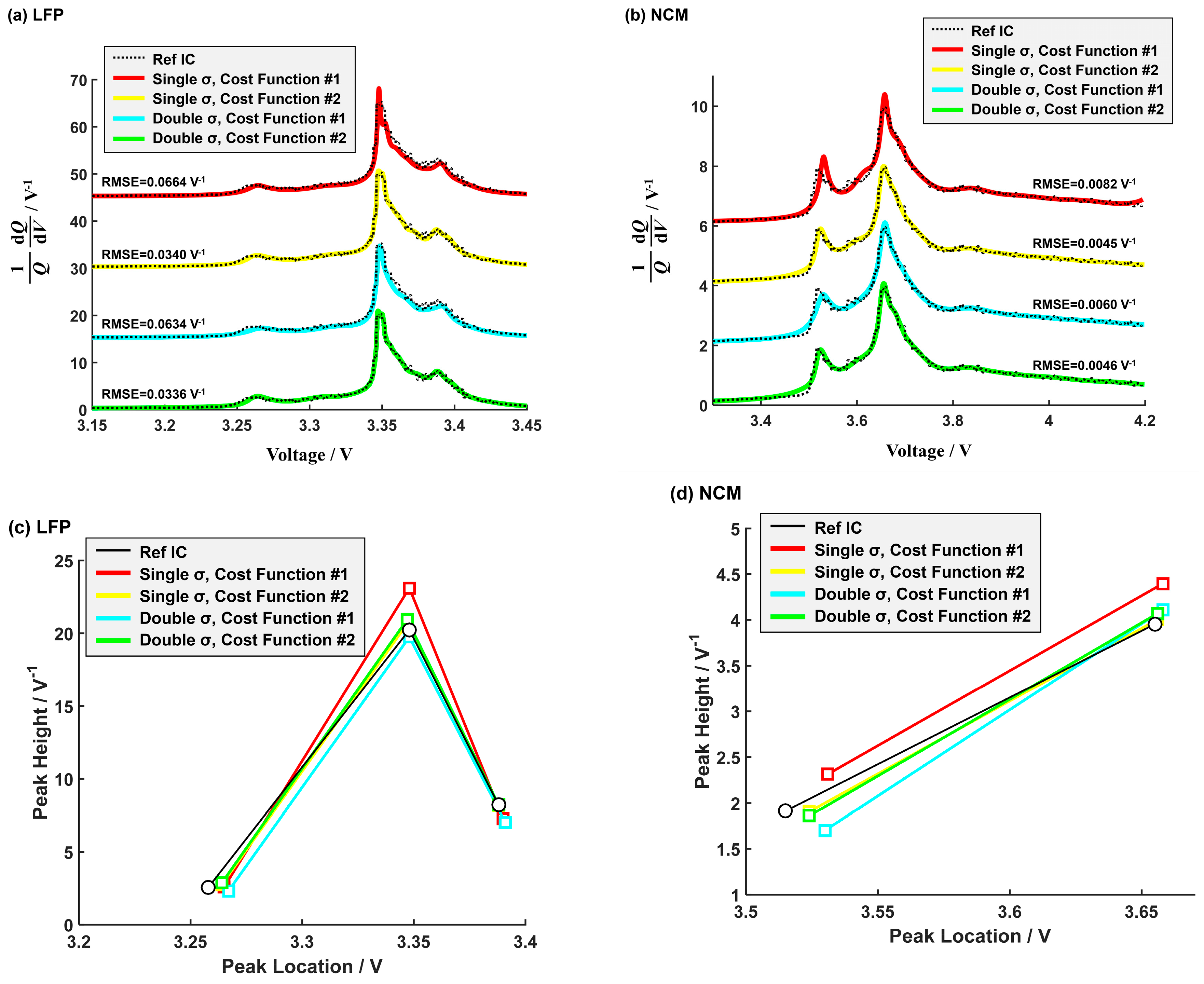
4.4. Changing the Cost Function to Improve the Accuracy of ICA Using the SVR Algorithm
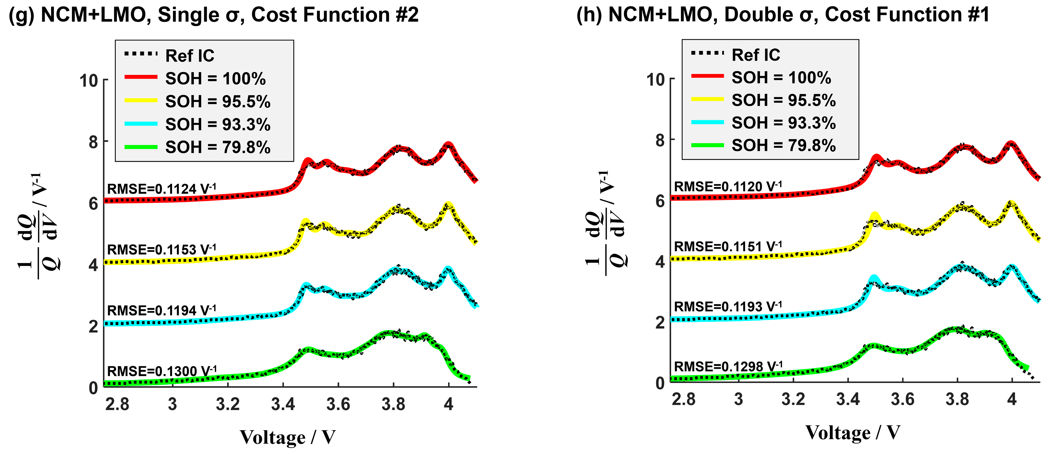
4.5. ICA for Characterizing the Degradation of Lithium-ion Batteries Using the SVR Algorithm
5. Conclusions
Author Contributions
Funding
Acknowledgments
Conflicts of Interest
References
- Hoog, J.D.; Jaguemont, J.; Abdel-Monem, M.; Bossche, P.V.D.; Mierlo, J.V.; Omar, N. Combining an electrothermal and impedance aging model to investigate thermal degradation caused by fast charging. Energies 2018, 11, 804. [Google Scholar] [CrossRef]
- Lai, X.; Zheng, Y.; Sun, T. A comparative study of different equivalent circuit models for estimating state-of-charge of lithium-ion batteries. Electrochimica Acta 2018, 259, 566–577. [Google Scholar] [CrossRef]
- Hu, X.; Martinez, C.M.; Yang, Y. Charging, power management, and battery degradation mitigation in plug-ion hybrid electric vehicles: A unified cost-optimal approach. Mech. Syst. Signal Process. 2017, 87, 4–16. [Google Scholar] [CrossRef]
- Kong, X.; Zheng, Y.; Ouyang, M.; Lu, L.; Li, J.; Zhang, Z. Fault diagnosis and quantitative analysis of micro-short circuits for lithium-ion batteries in battery packs. J. Power Sources 2018, 395, 358–368. [Google Scholar] [CrossRef]
- Zou, C.; Hu, X.; Wei, Z.; Wik, T.; Egardt, B. Electrochemical estimation and control for lithium-ion battery health-aware fast charging. IEEE Trans. Ind. Electron. 2018, 65, 6635–6645. [Google Scholar] [CrossRef]
- Huang, S.C.; Tseng, K.H.; Liang, J.W.; Chang, C.L.; Pecht, M.G. An online SOC and SOH model for lithium-ion batteries. Energies 2017, 10, 512. [Google Scholar] [CrossRef]
- Zheng, Y.; Ouyang, M.; Han, X.; Lu, L.; Li, J. Investigating the error sources of the online state of charge estimation methods for lithium-ion batteries in electric vehicles. J. Power Sources 2018, 377, 161–188. [Google Scholar] [CrossRef]
- Li, X.; Jiang, J.; Wang, L.Y.; Chen, D.; Zhang, Y.; Zhang, C. A capacity model based on charging process for state of health estimation of lithium ion batteries. Appl. Energy 2016, 177, 537–543. [Google Scholar] [CrossRef]
- Ouyang, M.; Feng, X.; Han, X.; Lu, L.; Li, Z.; He, X. A dynamic capacity degradation model and its applications considering varying load for a large format Li-ion battery. Appl. Energy 2016, 165, 48–59. [Google Scholar] [CrossRef]
- Yu, J.; Mo, B.; Tang, D.; Yang, J.; Wan, J.; Liu, J. Indirect state-of-health estimation for lithium-ion batteries under randomized use. Energies 2017, 10, 2012. [Google Scholar] [CrossRef]
- Hu, X.; Jiang, J.; Cao, D.; Egardt, B. Battery health prognosis for electric vehicles using sample entropy and sparse Bayesian predictive modeling. IEEE Trans. Ind. Electron. 2016, 63, 2645–2654. [Google Scholar] [CrossRef]
- Mathew, M.; Janhunen, S.; Rashid, M.; Long, F.; Fowler, M. Comparative analysis of lithium-ion battery resistance estimation techniques for battery management systems. Energies 2018, 11, 1490. [Google Scholar] [CrossRef]
- Bao, Y.; Dong, W.; Wang, D. Online internal resistance measurement application in lithium ion battery capacity and state of charge estimation. Energies 2018, 11, 1073. [Google Scholar] [CrossRef]
- Love, C.T.; Dubarry, M.; Reshetenko, T.; Devie, A.; Spinner, N.; Swider-Lyons, K.E.; Rocheleau, R. Lithium-ion cell fault detection by single-point impedance diagnostic and degradation mechanism validation for series-wired batteries cycled at 0 °C. Energies 2018, 11, 834. [Google Scholar] [CrossRef]
- Zou, Y.; Hu, X.; Ma, H.; Li, S.E. Combined state of charge and state of health estimation over lithium-ion battery cell cycle lifespan for electric vehicles. J. Power Sources 2015, 273, 793–803. [Google Scholar] [CrossRef]
- Shen, P.; Ouyang, M.; Lu, L.; Li, J.; Feng, X. The co-estimation of state of charge, state of health and state of function for lithium-ion batteries in electric vehicles. IEEE Trans. Veh. Technol. 2018, 67, 92–103. [Google Scholar] [CrossRef]
- Wu, T.H.; Moo, C.S. State-of-charge estimation with state-of-health calibration for lithium-ion batteries. Energies 2017, 10, 987. [Google Scholar] [CrossRef]
- Balewski, L.; Brenet, J.P. A new method for the study of the electrochemical reactivity of manganese dioxide. Electrochem. Technol. 1967, 5, 527–531. [Google Scholar]
- Dubarry, M.; Svoboda, V.; Hwu, R.; Liaw, B.Y. Incremental capacity analysis and close-to-equilibrium OCV measurements to quantify capacity fade in commercial rechargeable lithium batteries. Electrochem. Solid-State Lett. 2006, 9, A454–A457. [Google Scholar] [CrossRef]
- Dubarry, M.; Liaw, B.Y. Identify capacity fading mechanism in a commercial LiFePO4 cell. Electrochem. Technol. 2009, 194, 541–549. [Google Scholar] [CrossRef]
- Zhang, C.; Yan, F.; Du, C.; Kang, J.; Turkson, R.F. Evaluating the degradation mechanism and state of health of LiFePO4 lithium-ion batteries in real-world plug-ion hybrid electric vehicles application for different ageing paths. Energies 2017, 10, 110. [Google Scholar] [CrossRef]
- Han, X.; Ouyang, M.; Lu, L.; Li, J.; Zheng, Y.; Li, Z. A comparative study of commercial lithium ion battery cycle life in electrical vehicle: Aging mechanism identification. J. Power Sources 2014, 251, 38–54. [Google Scholar] [CrossRef]
- Dubarry, M.; Svoboda, V.; Hwu, R.; Liaw, B.Y. Capacity and power fading mechanism identification formo a commercial cell evaluation. J. Power Sources 2007, 165, 566–572. [Google Scholar] [CrossRef]
- Gao, Y.; Jiang, J.; Zhang, C.; Zhang, W.; Ma, Z.; Jiang, Y. Lithium-ion battery aging mechanisms and life model under different charging stresses. J. Power Sources 2017, 356, 103–114. [Google Scholar] [CrossRef]
- Jiang, Y.; Jiang, J.; Zhang, C.; Zhang, W.; Gao, Y.; Guo, Q. Recognition of battery aging variations for LiFePO4 batteries in 2nd use applications combining incremental capacity analysis and statistical approaches. J. Power Sources 2017, 360, 180–188. [Google Scholar] [CrossRef]
- Feng, X.; Li, J.; Ouyang, M.; Lu, L.; Li, J.; He, X. Using probability density function to evaluate the state of health of lithium-ion batteries. J. Power Sources 2013, 232, 209–218. [Google Scholar] [CrossRef]
- Weng, C.; Feng, X.; Sun, J.; Peng, H. State-of-health monitoring of lithium-ion battery modules and packs via incremental capacity peak tracking. Appl. Energy 2016, 180, 360–388. [Google Scholar] [CrossRef]
- Christopheren, J.P.; Shaw, S.R. Using radial basis functions to approximate battery differential capacity and differential voltage. J. Power Sources 2010, 195, 1225–1234. [Google Scholar] [CrossRef]
- Samad, N.A.; Kim, Y.; Siegel, J.B.; Stefanopoulou, A.G. Battery capacity fading estimation using a force-based incremental capacity analysis. J. Electrochem. Soc. 2016, 163, A1584–A1594. [Google Scholar] [CrossRef]
- Savitzky, A.; Golay, M.J.E. Smoothing and differentiation of data by simplified least squared procedures. Anal. Chem. 1964, 36, 1627–1639. [Google Scholar] [CrossRef]
- He, Y.; Shen, J.; Shen, J.; Ma, Z. Embedding monotonicity in the construction of polynomial open-circuit voltage model for lithium-ion batteries: A semi-infinite programming formulation approach. Ind. Eng. Chem. Res. 2015, 54, 3167–3174. [Google Scholar] [CrossRef]
- Hu, X.; Li, S.E.; Yang, Y. Advanced machine learning approach for lithium-ion battery state estimation in electric vehicles. IEEE Trans. Transport. Electrif. 2016, 2, 140–149. [Google Scholar] [CrossRef]
- Zhang, C.; Jiang, J.; Zhang, W.; Wang, Y.; Sharkh, S.M.; Xiong, R. A novel data-driven fast capacity estimation of spent electric vehicle lithium-ion batteries. Energies 2014, 7, 8076–8094. [Google Scholar] [CrossRef]
- Peng, Y.; Hou, Y.; Song, Y.; Pang, J.; Liu, D. Lithium-ion battery prognostics with hybrid Gaussian process function regression. Energies 2018, 11, 1420. [Google Scholar] [CrossRef]
- Weng, C.; Cui, Y.; Sun, J.; Peng, H. On-board state of health monitoring of lithium-ion batteries using incremental capacity analysis with support vector regression. J. Power Sources 2013, 235, 36–44. [Google Scholar] [CrossRef]
- Ren, D.; Lu, L.; Ouyang, M.; Feng, X.; Li, J.; Han, X. Degradation identification of individual components in the LiyNi1/3Co1/3Mn1/3O2-LiyMn2O4 blended cathode for large format lithium ion battery. Energy Procedia 2017, 105, 2698–2704. [Google Scholar] [CrossRef]
- Drucker, H.; Burges, C.J.C.; Kaufman, L.; Smola, A.; Vapnik, V. Support vector regression machines. In Proceedings of the 9th International Conference on Neural Information Processing Systems, Denver, CO, USA, 3–5 December 1996; pp. 155–161. [Google Scholar]


| Cell | Cathode | Anode | Capacity (Ah) | Voltage (V) | Current | Institute | Refference |
|---|---|---|---|---|---|---|---|
| A | LFP | C | 1.1 | 3.0–3.55 | 1/2 C CHA | UoM | [35] |
| B | NCM | C | 48 | 3.0–4.2 | 1/3 C CHA | THU | [26] |
| C | LFP | C | 60 | 2.75–3.6 | 1/3 C CHA | THU | [26] |
| D | NCM + LMO | C | 20 | 2.5–4.2 | 1/2 C DIS | THU | [36] |
| Algorithm | Fitting Accuracy | y = f(x) | y’ = f’(x) | Further Aging ICA | |
|---|---|---|---|---|---|
| σ | Cost Function | ||||
| Single σ | #1 | Fair | Explicit | Explicit | Not Recommended |
| Single σ | #2 | Better | No | Explicit | Recommended |
| Double σ | #1 | Good | Explicit | Explicit | Recommended |
| Double σ | #2 | Better | No | Explicit | Recommended |
| Cell | Cathode | SOH | Characteristic Peak | |||||||
|---|---|---|---|---|---|---|---|---|---|---|
| Reference IC (Linear Approximation) | Relative Error | |||||||||
| SVR Single σ Cost Function #2 | SVR Double σ Cost Function #1 | SVR Double σ Cost Function #2 | ||||||||
| Location /V | Height /V−1 | Location | Height | Location | Height | Location | Height | |||
| A | LFP | 100% | 3.388 | 8.205 | 0% | −0.23% | +0.09% | −14.45% | 0% | +0.04% |
| 99.7% | 3.388 | 7.344 | +0.03% | +0.07% | +0.12% | −16.60% | +0.03% | −0.07% | ||
| 97.8% | 3.388 | 6.328 | +0.06% | +0.03% | +0.09% | −14.84% | +0.06% | −0.30% | ||
| 95.7% | 3.392 | 5.573 | +0.18% | −4.25% | 0% | −9.54% | +0.15% | −4.19% | ||
| B | NCM | 100% | 3.655 | 3.953 | +0.03% | +1.24% | +0.08% | +3.92% | +0.03% | +2.93% |
| 97.6% | 3.655 | 3.731 | +0.05% | +2.68% | +0.08% | +4.90% | 0% | +3.03% | ||
| 90.5% | 3.660 | 3.563 | +0.08% | +0.93% | +0.11% | +4.15% | 0% | +0.28% | ||
| 78.8% | 3.675 | 3.117 | +0.03% | +0% | +0.05% | +2.44% | 0% | +0.19% | ||
| C | LFP | 100% | 3.394 | 11.02 | +0.03% | +0.73% | +0.09% | +15.70% | +0.09% | +6.62% |
| 91.1% | 3.390 | 10.77 | +0.06% | +3.25% | +0.15% | −6.78% | +0.24% | −0.74% | ||
| 85.3% | 3.390 | 8.873 | +0.18% | +8.58% | +0.21% | −1.78% | +0.09% | +5.42% | ||
| 78.7% | 3.398 | 6.344 | −0.15% | +5.74% | 0% | −6.45% | −0.09% | −6.76% | ||
| D | NCM+LMO | 100% | 3.990 | 1.875 | +0.23% | +1.39% | +0.13% | −0.32% | +0.28% | −2.29% |
| 95.5% | 3.990 | 1.931 | +0.20% | +0.73% | +0.13% | −1.40% | +0.25% | −1.50% | ||
| 93.3% | 3.990 | 1.823 | +0.18% | +1.43% | +0.25% | −1.26% | +0.25% | +0.66% | ||
| 79.8% | 3.916 | 1.670 | −0.08% | +0.72% | −0.38% | −2.51% | +0.20% | −0.30% | ||
| Cell | Cathode | SOH | Integrated Area Near the Peak | SVR Single σ + Cost Function #2 Relative Error | SVR Double σ + Cost Function #1 Relative Error |
|---|---|---|---|---|---|
| A | LFP | 100% | [3.380, 3.400] V | +0.61% | −9.96% |
| 99.7% | [3.380, 3.400] V | −0.76% | −9.89% | ||
| 97.8% | [3.380, 3.400] V | −0.90% | −8.65% | ||
| 95.7% | [3.380, 3.400] V | +1.85% | −10.65% | ||
| B | NCM | 100% | [3.620, 3.750] V | −0.34% | −0.15% |
| 97.6% | [3.620, 3.750] V | −0.52% | −0.14% | ||
| 90.5% | [3.620, 3.750] V | 0.39% | +0.10% | ||
| 78.8% | [3.620, 3.750] V | 0.68% | +0.21% | ||
| C | LFP | 100% | [3.380, 3.410] V | +0.40% | +0.78% |
| 91.1% | [3.380, 3.410] V | −0.33% | −2.62% | ||
| 85.3% | [3.380, 3.410] V | −1.99% | −3.45% | ||
| 78.7% | [3.380, 3.410] V | −2.76% | −5.29% | ||
| D | NCM+LMO | 100% | [3.910, 4.050] V | +0.49% | +0.04% |
| 95.5% | [3.910, 4.050] V | +0.25% | +0.19% | ||
| 93.3% | [3.910, 4.050] V | −0.14% | −0.21% | ||
| 79.8% | [3.880, 4.020] V | −0.82% | −0.31% |
© 2018 by the authors. Licensee MDPI, Basel, Switzerland. This article is an open access article distributed under the terms and conditions of the Creative Commons Attribution (CC BY) license (http://creativecommons.org/licenses/by/4.0/).
Share and Cite
Feng, X.; Weng, C.; He, X.; Wang, L.; Ren, D.; Lu, L.; Han, X.; Ouyang, M. Incremental Capacity Analysis on Commercial Lithium-Ion Batteries using Support Vector Regression: A Parametric Study. Energies 2018, 11, 2323. https://doi.org/10.3390/en11092323
Feng X, Weng C, He X, Wang L, Ren D, Lu L, Han X, Ouyang M. Incremental Capacity Analysis on Commercial Lithium-Ion Batteries using Support Vector Regression: A Parametric Study. Energies. 2018; 11(9):2323. https://doi.org/10.3390/en11092323
Chicago/Turabian StyleFeng, Xuning, Caihao Weng, Xiangming He, Li Wang, Dongsheng Ren, Languang Lu, Xuebing Han, and Minggao Ouyang. 2018. "Incremental Capacity Analysis on Commercial Lithium-Ion Batteries using Support Vector Regression: A Parametric Study" Energies 11, no. 9: 2323. https://doi.org/10.3390/en11092323
APA StyleFeng, X., Weng, C., He, X., Wang, L., Ren, D., Lu, L., Han, X., & Ouyang, M. (2018). Incremental Capacity Analysis on Commercial Lithium-Ion Batteries using Support Vector Regression: A Parametric Study. Energies, 11(9), 2323. https://doi.org/10.3390/en11092323