A Hybrid DA-PSO Optimization Algorithm for Multiobjective Optimal Power Flow Problems

Abstract

In this paper, a hybrid optimization algorithm is proposed to solve multiobjective optimal power flow problems (MO-OPF) in a power system. The hybrid algorithm, named DA-PSO, combines the frameworks of the dragonfly algorithm (DA) and particle swarm optimization (PSO) to find the optimized solutions for the power system. The hybrid algorithm adopts the exploration and exploitation phases of the DA and PSO algorithms, respectively, and was implemented to solve the MO-OPF problem. The objective functions of the OPF were minimization of fuel cost, emissions, and transmission losses. The standard IEEE 30-bus and 57-bus systems were employed to investigate the performance of the proposed algorithm. The simulation results were compared with those in the literature to show the superiority of the proposed algorithm over several other algorithms; however, the time computation of DA-PSO is slower than DA and PSO due to the sequential computation of DA and PSO.

1. Introduction

For the past few decades, the optimal power flow (OPF) problem has played an essential role in studying the economy terms of power systems [1,2]. The OPF problem is a nonlinear, nonconvex, large-scale, and static programming problem [3] that optimizes selected objective functions while satisfying a set of equality and inequality constraints. The power balance equations are the equality constraints, and the limits of state and control variables are the inequality constraints of the OPF problem. The state variables consist of slack bus active power generation, load bus voltages, reactive power generation, and apparent power flow. The control variables involve active power generation except at slack bus, generator bus voltages, tap ratios of transformers, and reactive powers of shunt compensation capacitors. In recent years, because of the rise in fuel cost, which increases generation cost, fuel cost has become the objective function to be optimized in the OPF problem. Moreover, due to the release of emissions from thermal power plants into the atmosphere, emissions are yet another concern for power system operation and planning [4]. At the same time, because the demand for electricity has outpaced the expansion of transmission capacity, the inadequate reactive power sources of power systems have increased losses in transmission lines. Thus, emissions and transmission losses must also be considered as part of the objective functions of the OPF problem.

To solve the OPF problem, several traditional optimization techniques, such as nonlinear programming [5], quadratic programming [6], and the interior point method [7], have been successfully applied. However, these algorithms’ nonlinear characteristics make them impractical to use in practical systems. The nonlinear characteristics may cause the obtained solutions to be trapped in local optima, and these algorithms require an enormous amount of computational effort and time. Therefore, many optimization methods need to be improved to overcome these shortcomings [8,9]. Recently, several population-based optimization algorithms, including the OPF problem, have been employed to solve a complex constrained optimization problem in the field of power systems. Some of the other proposed techniques include the genetic algorithm (GA) [10], tabu search (TS) [11], differential evolution (DE) [12], evolutionary programming (EP) [13], probabilistic optimal power-flow (P-OPF) [14], preventive security-constrained power flow optimization [15], ant colony optimization (ACO) [16], grey wolf optimizer (GWO) [17], artificial bee colony (ABC) [18], particle swarm optimization (PSO) [19], and the dragonfly algorithm (DA) [20]. Even with the successful optimization of single-objective population-based optimization techniques, minimizing only one objective function is not sufficient in the power system because there are many problems, such as fuel cost, emissions, and transmission losses, which also need to be minimized. Consequently, many objective functions should be considered because this is a multi objective optimization problem. Since there are three independent objective functions in this study (i.e., fuel cost, emissions, and transmission losses), the number of incompatible optimal solutions between the objective functions is infinite, and these optimal solutions are called Pareto optimal solutions [21].

Several optimization algorithms have been proposed and applied to solve the multiobjective OPF (MO-OPF) problem by many researchers. One of these methods was carried out by converting the multiobjective problem into a single-objective problem and then solving the problem by using a single-objective optimizer. However, this method has some drawbacks, such as the limitation of the available choices, the need for weights for each objective, and the requirement of multiple optimizer runs. To overcome these weaknesses, many researchers have proposed multiobjective evolutionary algorithms, such as the improved strength Pareto evolutionary algorithm (ISPEA2) [22], hybrid modified particle swarm optimization-shuffle frog leaping algorithms (HMPSO-SFLA) [23], modified teaching–learning-based optimization (MTLBO) [24], GWO [17], DE [17], multiobjective modified imperialist competitive algorithm (MOMICA) [25], differential search algorithm (DSA) [26], modified shuffle frog leaping algorithm (MSFLA) [27], modified Gaussian bare-bones multiobjective imperialist competitive algorithm (MGBICA) [28], multiobjective harmony search (MOHS) [29], adaptive real coded biogeography-based optimization (ARCBBO) [30], multiobjective differential evolution algorithm (MO-DEA) [31], hybrid modified imperialist competitive algorithm and teaching–learning algorithm (MICA-TLA) [32], etc., to successfully solve the OPF problem. In the past few decades, various well-proposed multiobjective evolutionary algorithms have been successfully applied and improved in many applications; however, most of them have not been extensively investigated in the OPF problem. Moreover, improving the search performance of the multiobjective evolutionary algorithm for solving the OPF problem is also important. In this paper, a hybrid DA-PSO algorithm is proposed to deal with the MO-OPF problem. The concept of the hybrid algorithm is the combination of the exploration and exploitation phases of the DA and PSO algorithms, respectively. The performance of the proposed algorithm was evaluated on the standard IEEE 30-bus and IEEE 57-bus power systems. Three different objective functions—fuel cost, emissions, and transmission losses—were individually and simultaneously considered as parts of the objective function in the OPF problem. The obtained results were compared with other evolutionary algorithms and the traditional DA and PSO.

The rest of the article is classified into five sections as follows. Section 2 introduces the formulation and constraints of the multiobjective optimization. In Section 3, the traditional DA and PSO are explained, and Section 4 depicts the concept of the proposed algorithm. Section 5 presents the optimization results and the comparisons between the solutions from the proposed algorithm and the solution from other algorithms based on IEEE 30-bus and IEEE 57-bus systems. Finally, in Section 6, the conclusions of the simulation results of the proposed algorithm are described.

2. Problem Formulation and Constraints for Multi Objective Optimization for OPF

Multi-objective optimization is a model that optimizes more than one objective function to find optimal control variables while simultaneously satisfying equality and inequality constraints. The compromised solutions, nondominated solutions, which have more than one optimal solution between each objective, are the optimal solutions referred to as the Pareto front. The multiobjective problem is mathematically formulated as follows:

$$\min \mathit{f}=\{{\mathit{f}}_1(\mathit{x},\mathit{u}),{\mathit{f}}_2(\mathit{x},\mathit{u}),\dots ,{\mathit{f}}_{{\mathit{N}}_{obj}}(\mathit{x},\mathit{u})\}$$

(1)

subject to

$$g(\mathit{x},\mathit{u})=0$$

(2)

$$h(\mathit{x},\mathit{u})\le 0$$

(3)

where f is a vector of objective functions to be optimized, N_obj is the number of objective functions, g(x,u) are the equality constraints, and h(x,u) are the inequality constraints.

x is a vector of state variables including slack bus active power, load bus voltages, generator reactive powers, and apparent power flows, expressed as follows:

$$\mathit{x}=[P_{gslack},V_{L1},\dots ,V_{L{N}_L},Q_{g1}\dots Q_{g{N}_{gen}},S_{l1}\dots S_{l{N}_l}]$$

(4)

where P_gslack is the active power generation at slack bus, V_Li is the load voltage at bus i, N_L is number of load buses, Q_gi is the reactive power generation at bus i, N_gen is the number of total generators, S_li is the apparent power flow at branch i, and N_l is the number of transmission lines.

u is a vector of control variables consisting of active power generations except at slack bus, generator bus voltages, transformer tap ratios, and reactive powers of shunt compensation capacitors, expressed as:

$$\mathit{u}=[P_{gi;i\in P{V}_{bus}}\dots P_{g{N}_{gen}},V_{g1},\dots ,V_{g{N}_{gen}},T_1\dots T_{N_{tran}},Q_{c1}\dots Q_{c{N}_{cap}}]$$

(5)

where P_gi is the active power generation at bus i, PV_bus is the set of generator buses except at slack bus, V_gi is the generator bus voltage at bus i, T_i is the transformer tap ratio at bus i, N_tran is the number of transformer taps, Q_ci is the shunt compensation capacitor at bus i, and N_cap is the number of compensation capacitors.

2.1. Objective Functions

In this study, the objective functions of the OPF, consisting of fuel cost, emissions, and transmission line losses, are considered as shown below.

2.1.1. Fuel Cost

The total fuel cost of the generators is considered to be minimized and is given as follows:

$$f_C(\mathit{x},\mathit{u})={\displaystyle \sum _{i=1}^{N_{gen}}(a_i{P}_{gi}^2+b_i{P}_{gi}+c_i)}$$

(6)

where f_C is the total fuel cost of generators function ($/h), and a_i, b_i and c_i are the fuel cost coefficients of the ith generator units.

2.1.2. Emissions

The emissions function can be represented as the sum of all considered emission types, such as sulphur oxides (SO_x), nitrogen oxides (NO_x), thermal emission, etc. However, in the present study, two important emission types, NO_x and SO_x, are taken into account, as expressed below:

$$f_E(\mathit{x},\mathit{u})={\displaystyle \sum _{i=1}^{N_{gen}}({\gamma }_i{P}_{gi}^2+{\beta }_i{P}_{gi}+{\alpha }_i+{\xi }_i\exp ({\lambda }_i{P}_{gi}))}$$

(7)

where f_E is the total emission generations function (ton/h), and γ_i, β_i, α_i, ζ_i and λ_i are emission coefficients of the ith generator units.

2.1.3. Transmission Line Losses

The system active power loss in the transmission line is formulated as follows:

$$f_L(\mathit{x},\mathit{u})={\displaystyle \sum _{k=1}^{N_l}{g}_k(V_i^2+V_j^2-2V_i{V}_j\cos ({\theta }_{ij}))}$$

(8)

where f_L is the total transmission loss function (MW), g_k is the conductance of the kth line, V_i is the voltage at bus i, V_j is the voltage at bus j, and θ_ij is the voltage phase angle difference between buses i and j.

2.2. Constraints

2.2.1. Equality Constraints

The OPF equality constraints are the active and reactive power balance constraints, as follows:

$$P_{gi}-P_{di}={\displaystyle \sum _{j=1}^{N_{bus}}{V}_i{V}_j(G_{ij}\cos ({\theta }_{ij})+B_{ij}\sin ({\theta }_{ij}))}$$

(9)

$$Q_{gi}-Q_{di}={\displaystyle \sum _{j=1}^{N_{bus}}{V}_i{V}_j(G_{ij}\sin ({\theta }_{ij})-B_{ij}\cos ({\theta }_{ij}))}$$

(10)

where P_di is the active power demand at bus i, N_bus is the number of buses, G_ij is the transfer conductance between buses i and j, B_ij is the transfer susceptance between buses i and j, and Q_di is the reactive power demand at bus i.

2.2.2. Inequality Constraints

$$P_{gi\min }\le P_{gi}\le P_{gi\max }i=1,2,\dots ,N_{gen}$$

(11)

$$Q_{gi\min }\le Q_{gi}\le Q_{gi\max }i=1,2,\dots ,N_{gen}$$

(12)

$$V_{gi\min }\le V_{gi}\le V_{gi\max }i=1,2,\dots ,N_{gen}$$

(13)

$$\left|S_{li}\right|\le S_{li\max }$$

(14)

$$V_{Li\min }\le V_{Li}\le V_{Li\max }i=1,2,\dots ,N_L$$

(15)

$$Q_{ci\min }\le Q_{ci}\le Q_{ci\max }i=1,2,\dots ,N_{cap}$$

(16)

$$T_{i\min }\le T_i\le T_{i\max }i=1,2,\dots ,N_{tran}$$

(17)

where P_gimin and P_gimax are the minimum and maximum active power generations at bus i, respectively, Q_gimin and Q_gimax are the minimum and maximum reactive power generations at bus i, respectively, V_gimin, V_gimax are the minimum and maximum generator voltage at bus i, respectively, S_limax is the maximum apparent power flow at branch i, V_Limin, V_Limax are the minimum and maximum load voltage at bus i, respectively, Q_cimin and Q_cimax are the minimum and maximum shunt compensation capacitor at bus i, respectively, T_imin, T_imax are the minimum and maximum transformer tap-ratio at bus i, respectively.

2.2.3. Constraints Handling

The inequality of dependent variables, including slack bus active power generation, load bus voltage magnitudes, reactive power generations, and apparent power flows, are integrated into the penalized objective function to maintain these variables within their limits and to refuse infeasible solutions. The penalty function can be expressed as follows [27]:

$$\begin{gathered} \mathit{J}(\mathit{x},\mathit{u})=\mathit{f}(\mathit{x},\mathit{u})+K_P{(P_{gslack}-P_{gslack}^{\lim })}^2+K_V{\displaystyle \sum _{i=1}^{N_{load}}{(V_{Li}-V_{Li}^{\lim })}^2} \\ +K_Q{\displaystyle \sum _{i=1}^{N_{line}}(Q_{gi}-Q_{gi}^{\lim }}{)}^2+K_S{\displaystyle \sum _{i=1}^{N_{line}}{(S_{Li}-S_{Li}^{\max })}^2} \end{gathered}$$

(18)

where J(x,u) is the penalized objective function, K_p, K_Q, K_V and K_s are the penalty factors, and x^lim is the limit value of the dependent variables, determined as follows:

$$x^{\lim }=\{\begin{array}{c}{x}^{\max }\\ x\\ x^{\min }\end{array}\begin{array}{c}if\\ if\\ if\end{array}\begin{array}{c}x>x^{\max }\\ x^{\min }<x<x^{\max }\\ x<x^{\min }\end{array}$$

(19)

3. Related Optimization Techniques

3.1. DA

DA is a metaheuristic algorithm which was inspired by the static and dynamic swarming behaviors of dragonflies in nature [33]. Dragonflies swarm for two goals: Hunting (static swarm) and migration (dynamic swarm). In the dynamic swarm, many dragonflies swarm when roaming over long distances and different areas, which is the purpose of the exploration phase. In the static swarm, dragonflies move in larger swarms and along one direction with local movements and sudden changes in the flying path, which is suitable in the exploitation phase.

The behavior of dragonflies can be represented through five principles, which are separation, alignment, cohesion, attraction to a food source, and distraction of an enemy. These five behaviors are described and calculated as follows:

Separation, which is the avoidance of the static crashing of individuals into other individuals in the neighborhood, is calculated by Equation (20).

$${\mathit{S}}_{\mathit{i}}=-{\displaystyle \sum _{j=1}^N\mathit{X}-{\mathit{X}}_{\mathit{j}}}$$

(20)

where S_i is the separation of the ith individual, N is the number of neighboring individuals, X is the position of the current individual, and X_j is the position of jth neighboring individual.

Alignment, which refers to the velocity matching of individuals to the velocity of others in the neighborhood, is computed by Equation (21).

$${\mathit{A}}_{\mathit{i}}=\frac{{\displaystyle {\sum }_{j=1}^N{\mathit{V}}_{\mathit{j}}}}{N}$$

(21)

where A_i is the alignment of the ith individual, and V_j is the velocity of jth neighboring individual.

Cohesion, which is the propensity of individuals towards the center of mass of the neighborhood, is formulated by Equation (22).

$${\mathit{C}}_{\mathit{i}}=\frac{{\displaystyle {\sum }_{j=1}^N{\mathit{X}}_{\mathit{j}}}}{N}-\mathit{X}$$

(22)

where C_i is the cohesion of the ith individual

Attraction towards a food source computed by Equation (23), should be the main objective of any swarm to survive.

$${\mathit{F}}_{\mathit{i}}={\mathit{X}}^{+}-\mathit{X}$$

(23)

where F_i is the food source of the ith individual, and X⁺ is the position of the food source.

Distraction of an enemy, which is computed by Equation (24), is another survival objective of the swarm.

$${\mathit{E}}_{\mathit{i}}={\mathit{X}}^{-}+\mathit{X}$$

(24)

where E_i is the position of enemy of the ith individual, and X⁻ is the position of the enemy source.

To simulate the movement of artificial dragonflies and update their positions, step vector (ΔX) and position vector (X) are considered. The step vector represents the direction of the movement of the artificial dragonflies and is formulated as follows:

$$\mathbf{\Delta }{\mathit{X}}^{\mathit{t}+1}=(s{\mathit{S}}_{\mathit{i}}+a{\mathit{A}}_{\mathit{i}}+c{\mathit{C}}_{\mathit{i}}+f{\mathit{F}}_{\mathit{i}}+e{\mathit{E}}_{\mathit{i}})+{\omega }^t\mathbf{\Delta }{\mathit{X}}^{\mathit{t}}$$

(25)

where ΔX^{t + 1} is the step vector at iteration t + 1, ΔX^t is the step vector at iteration t, s, a, c, f and e are the separation weight, alignment weight, cohesion weight, food factor and enemy factor, respectively, and ω^t is the inertia weight factor at iteration t and is calculated by Equation (26).

$${\omega }^t={\omega }_{\max }-\frac{{\omega }_{\max }-{\omega }_{\min }}{Ite{r}_{\max }}\times Iter$$

(26)

where ω_max and ω_min are set to 0.9 and 0.4, respectively, Iter is the iteration, and Iter_max is the maximum iteration.

The position of the artificial dragonflies can be updated by the following equation:

$${\mathit{X}}^{\mathit{t}+1}={\mathit{X}}^{\mathit{t}}+\mathbf{\Delta }{\mathit{X}}^{\mathit{t}+1}$$

(27)

where X^{t+ 1} is the position at iteration t + 1, and X^t is the position at iteration t.

When the search space does not have a neighboring solution, the artificial dragonflies need to move around the search space by applying random walk (Levy flight) to improve their stochastic behavior. So, in this case, the position of the dragonflies can be calculated by Equation (28).

$${\mathit{X}}^{\mathit{t}+1}={\mathit{X}}^{\mathit{t}}+\mathit{L}\mathit{e}\mathit{v}\mathit{y}(d)\times {\mathit{X}}^{\mathit{t}}$$

(28)

where d is the dimension of the position vectors, and the Levy is the Levy flight which is computed by Equation (29).

$$\mathit{L}\mathit{e}\mathit{v}\mathit{y}(d)=0.01\times \frac{r_1\times \sigma }{{\left|r_2\right|}^{\frac{1}{\beta }}}$$

(29)

where r₁ and r₂ are two uniform random values in a range of [0, 1], and σ is calculated by Equation (30).

$$\sigma ={\left(\frac{\mathsf{\Gamma }(1+\beta )\times \sin \left(\frac{\pi \beta }{2}\right)}{\mathsf{\Gamma }\left(\frac{1+\beta }{2}\right)\times \beta \times 2^{\left(\frac{\beta -1}{2}\right)}}\right)}^{1/\beta }$$

(30)

where β is the constant (which is equal to 1.5 in this work), and $\mathsf{\Gamma }(x)=(x-1)!$.

3.2. PSO

PSO is a population-based stochastic global optimization technique which was first introduced by Eberhart and Kennedy [34]. The idea of PSO came from the flocking behavior of birds or the schooling of fishes in their food hunting. In the PSO system, the population moves around a multidimensional search space where each particle represents a possible solution. Each particle contains the information of control variables and is associated with a fitness value that indicates its performance in the fitness space. Each particle i consists of its position X_i = (x_i,1, x_i,2, …, x_i,Nvar), where Nvar represents the number of control variables, velocity V_i = (v_i,1, v_i,2, …, v_i,Nvar) and personal best experience X_pbesti = (x_pbesti,1, x_pbesti,2, …, x_pbesti,Nvar), and a swarm has a global best experience X_gbest = (x_gbest1, x_gbest2, …, x_gbestNvar). During each iteration, each particle moves in the direction of its own personal best position provided so far as well as in the direction of the global best position obtained so far by particles in the swarm. The particles are operated according to the equations expressed as follows:

$${\mathit{V}}_{\mathit{i}}^{\mathit{t}+1}={\omega }^t\times {\mathit{V}}_{\mathit{i}}^{\mathit{t}}+C_1\times ran{d}_1\times ({\mathit{X}}_{\mathit{p}\mathit{b}\mathit{e}\mathit{s}{\mathit{t}}_{\mathit{i}}}^{\mathit{t}}-{\mathit{X}}_{\mathit{i}}^{\mathit{t}})+C_2\times ran{d}_2\times ({\mathit{X}}_{\mathit{g}\mathit{b}\mathit{e}\mathit{s}\mathit{t}}^{\mathit{t}}-{\mathit{X}}_{\mathit{i}}^{\mathit{t}})$$

(31)

$${\mathit{X}}_{\mathit{i}}^{\mathit{t}+1}={\mathit{X}}_{\mathit{i}}^{\mathit{t}}+{\mathit{V}}_{\mathit{i}}^{\mathit{t}+1}$$

(32)

where V_i^{t+ 1} is the velocity of particle i at iteration t + 1, V_i^t is the velocity of particle i at iteration t, C₁ and C₂ are two positive acceleration constants, rand₁ and rand₂ are two uniform random values in a range of [0, 1], X^t_pbesti is the personal best position of particle i at iteration t, X_i^t is the position of particle i at iteration t, X^t_gbest is the global best position among all particles at iteration t, and X_i^{t+ 1} is the position of particle i at iteration t + 1.

4. Proposed Hybrid DA-PSO Optimization Algorithm for MO-OPF Problem

Many optimization algorithms have been proposed to overcome the optimization problem of being trapped in the local optima while the algorithms try to find the best solution. PSO has been proven in several works from the literature to find the optimal solution in various problems [35,36,37,38]. Because of its equations in finding the optimal solution by using the best experience of the particles, PSO could quickly converge on the optimal solution, i.e., it is good at exploitation. However, PSO is sometimes still trapped in the local optima because it converges on the optimal solution too quickly. In other words, PSO is poor at exploration, which is an important task of the optimization process. In DA, it applies the Levy flight to improve the randomness and stochastic behavior when there is no neighboring dragonfly. This could significantly improve the exploration process of the algorithm. However, the best experience, which is the personal best, of dragonflies is not applied during the operation. This causes the DA to converge on the optimal solution very slowly and can sometimes cause it to be trapped in the local optima. To overcome these problems, a new algorithm is proposed which combines the prominent points of the DA and PSO algorithms, which are the exploration of DA and the exploitation of PSO. At first, the dragonflies in DA are initialized to explore the search space to find the area of the global solution. Then, the best position of DA is obtained. The obtained best position from DA is then substituted as the global best position in the PSO equation (Equation (31)). After that, the PSO algorithm, which is the exploitation phase, operates by using the global best position from DA, allowing it to provide the expected optimal solution. The velocity and position equations of PSO can be modified as follows:

$${\mathit{V}}_{\mathit{i}}^{\mathit{t}+1}={\omega }^t\times {\mathit{V}}_{\mathit{i}}^{\mathit{t}}+C_1\times ran{d}_1\times ({\mathit{X}}_{\mathit{p}\mathit{b}\mathit{e}\mathit{s}{\mathit{t}}_{\mathit{i}}}^{\mathit{t}}-{\mathit{X}}_{\mathit{i}}^{\mathit{t}})+C_2\times ran{d}_2\times ({\mathit{X}}_{\mathit{D}\mathit{A}}^{\mathit{t}+1}-{\mathit{X}}_{\mathit{i}}^{\mathit{t}})$$

(33)

$${\mathit{X}}_{\mathit{i}}^{\mathit{t}+1}={\mathit{X}}_{\mathit{i}}^{\mathit{t}}+{\mathit{V}}_{\mathit{i}}^{\mathit{t}+1}$$

(34)

where ${\mathit{X}}_{\mathit{D}\mathit{A}}^{\mathit{t}+1}$ is the best position obtained from DA at iteration t + 1.

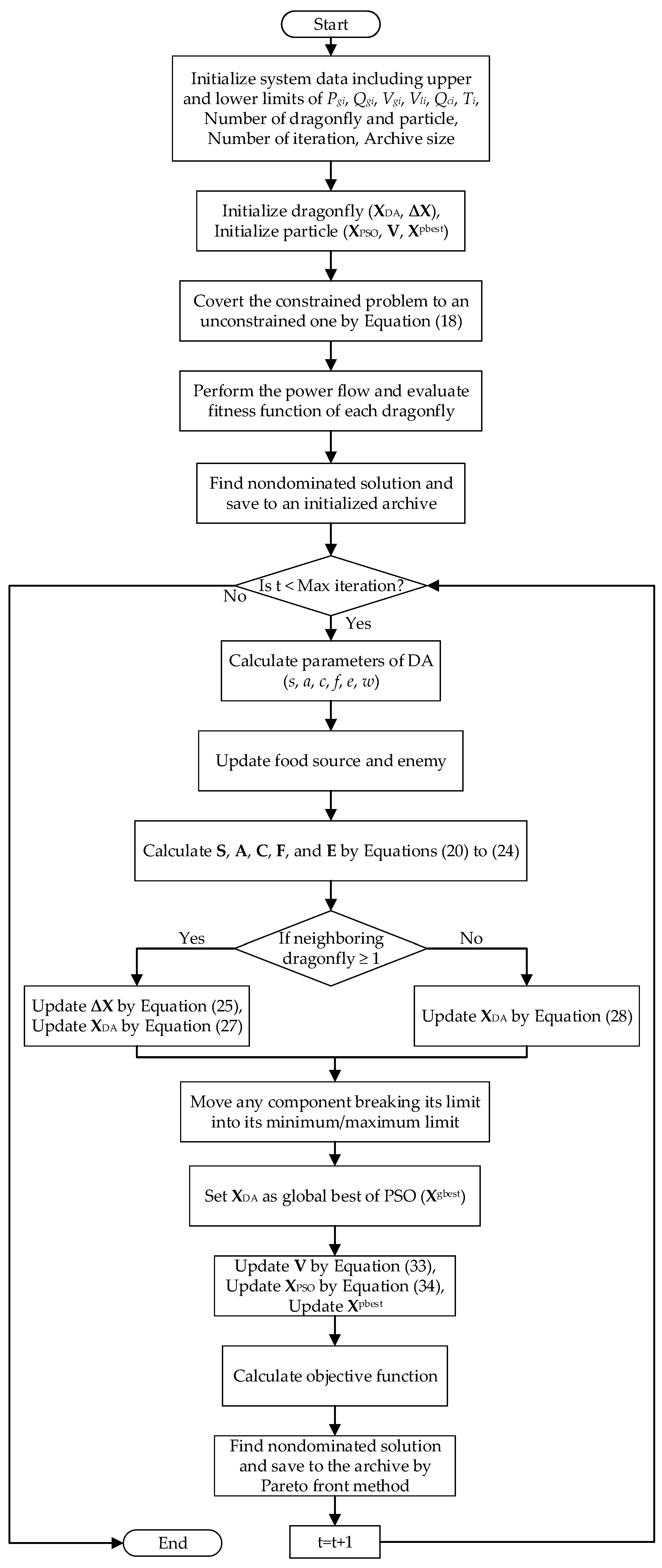
The application of the proposed DA-PSO algorithm for solving the MO-OPF problem can be described as follows:

Step 1.

Clarify the system data comprising the fuel cost coefficients of the generators, emission coefficients of the generators, initial values of generator active powers, initial values of generator bus voltages, initial values of transformer tap ratios, initial values of shunt compensation capacitors, upper limit of S_li, lower and upper limits of P_gi, Q_gi, V_gi, V_Li, Q_ci, and T_i, the parameters of DA and PSO, the number of dragonflies and particles, the number of iterations, and the archive size.

Step 2.

Generate the initial population of dragonflies and particles.

Step 3.

Convert the constrained multi objective problem to an unconstrained one by using Equation (18).

Step 4.

Perform the power flow and calculate the objective functions for the initial population of dragonflies.

Step 5.

Find the nondominated solutions and save them to the initial archive.

Step 6.

Set the fitness value of the initial population as the food source.

Step 7.

Calculate the parameters of DA (s, a, c, f, and e).

Step 8.

Update the food source and enemy of DA.

Step 9.

Calculate the S, A, C, F, and E by Equations (20)–(24).

Step 10.

Check if a dragonfly has at least one neighboring dragonfly, then update step vector (ΔX) and the position of dragonfly (X_DA) by Equations (25) and (27), respectively, and if each dragonfly has no neighboring dragonfly, then update X_DA by Equation (28) and set ΔX to be zero.

Step 11.

If any component of each population breaks its limit, then ΔX or X_DA of that population is moved into its minimum/maximum limit.

Step 12.

Set the best position obtained from DA as the global best of PSO (X^gbest).

Step 13.

Update the velocity of the particle (V) and the position of the particle (X_PSO) by Equations (33) and (34), respectively.

Step 14.

If any component of each population breaks its limit, then V or X_PSO of that population is moved into its minimum/maximum limit.

Step 15.

Calculate the objective functions of the new produced population.

Step 16.

Employ the Pareto front method to save the nondominated solutions to the archive and update the archive.

Step 17.

If the maximum number of iterations is reached, the algorithm is stopped; otherwise, go to step 7.

The flowchart of the DA-PSO algorithm for the MO-OPF problem is shown in Figure 1.

5. Simulation Results

To investigate the performance of the proposed algorithm, the IEEE 30-bus and IEEE 57-bus test systems were employed. The proposed algorithm operated for 30 independent runs for each test system. To validate the superiority of the proposed algorithm for solving the economic dispatch optimization problem, the results provided by the proposed algorithm were compared with those of other metaheuristic algorithms from the literature. In order to investigate both the single-objective optimization and multiobjective optimization, the simulation was divided into two cases. Single-objective optimization was evaluated in the first case. In the second case, multiobjective optimization to solve the MO-OPF by using the proposed DA-PSO algorithm was evaluated.

5.1. IEEE 30-Bus Test System

The proposed DA-PSO algorithm was applied to the IEEE 30-bus system to evaluate its performance. The IEEE 30-bus test system was composed of 6 generators at buses 1, 2, 5, 8, 11, and 13, 4 transformers between buses 6 and 9, buses 6 and 10, buses 4 and 12, and buses 27 and 28, and 41 transmission lines. The total system demand was 283.4 MW and 126.6 MVAR. The bus and branch data is given in [39]. The population number and the size of the Pareto archive were set to be 100 and 100, respectively.

5.1.1. Single-Objective OPF

To evaluate the performance of the proposed algorithm for solving the single-objective optimization, three different objective functions consisting of fuel cost, emissions, and transmission loss minimizations were individually considered as part of the objective function. The obtained results by the traditional DA, PSO, and the proposed DA-PSO algorithm for three individual objective functions are shown in

Table 1. Comparison of the simulation results from particle swarm optimization (PSO), dragonfly algorithm (DA), and DA-PSO for IEEE 30-bus system.

Variables	Best Fuel Cost			Best Emission			Best PLoss
	PSO	DA	DA-PSO	PSO	DA	DA-PSO	PSO	DA	DA-PSO
Pg1 (MW)	176.2376	176.5128	176.1861	64.1678	64.3407	64.0997	51.6974	51.5987	51.5893
Pg2 (MW)	48.8432	48.6955	48.8318	67.6692	67.5383	67.6295	80.0000	80.0000	80.0000
Pg3 (MW)	21.5184	21.4431	21.5119	50.0000	50.0000	50.0000	50.0000	50.0000	50.0000
Pg4 (MW)	22.1257	22.0995	22.0737	35.0000	35.0000	35.0000	35.0000	35.0000	35.0000
Pg5 (MW)	12.2000	12.0673	12.2005	30.0000	30.0000	30.0000	30.0000	40.0000	30.0000
Pg6 (MW)	12.0000	12.0091	12.0000	40.0000	40.0000	40.0000	40.0000	40.0000	40.0000
Vg1 (p.u.)	1.0500	1.0500	1.0500	1.0500	1.0500	1.0500	1.0500	1.0500	1.0500
Vg2 (p.u.)	1.0381	1.0379	1.0379	1.0459	1.0472	1.0459	1.0477	1.0476	1.0476
Vg3 (p.u.)	1.0110	1.0117	1.0109	1.0274	1.0309	1.0277	1.0292	1.0283	1.0292
Vg4 (p.u.)	1.0194	1.0197	1.0187	1.0353	1.0377	1.0350	1.0366	1.0342	1.0363
Vg5 (p.u.)	1.1000	1.1000	1.1000	1.1000	1.1000	1.1000	1.1000	1.0387	1.1000
Vg6 (p.u.)	1.0999	1.0842	1.0828	1.0852	1.0140	1.0713	1.0850	1.0606	1.0712
T6-9 (p.u.)	0.9973	1.0318	1.0166	1.0136	1.0017	1.0490	1.0153	1.1000	1.0482
T6-10 (p.u.)	0.9000	0.9004	0.9210	0.9000	1.1000	0.9000	0.9000	0.9000	0.9000
T4-12 (p.u.)	1.0157	0.9995	0.9980	1.0097	1.0003	0.9954	1.0105	0.9740	0.9962
T27-28 (p.u.)	0.9403	0.9501	0.9478	0.9518	1.0136	0.9609	0.9529	0.9647	0.9618
Qc10 (MVar)	28.6430	7.0219	10.0521	0.0000	0.0030	5.7174	7.0753	30.0000	5.2416
Qc24 (MVar)	0.0000	11.0974	10.6433	30.0000	16.6605	10.6333	17.0085	9.9534	10.6499
Fuel Cost ($/h)	802.5449	802.1299	802.1241	945.0484	944.9387	944.7159	968.1335	967.8979	967.8756
Emission (ton/h)	0.363619	0.364411	0.363494	0.204886	0.204861	0.204853	0.207294	0.207280	0.207279
PLoss (MW)	9.5249	9.4272	9.4041	3.4370	3.4790	3.3292	3.2974	3.1987	3.1893

. In

Table 2. Comparison of the results from DA-PSO and other algorithms when considering only fuel cost as part of the objective function for IEEE 30-bus system.

Algorithms	Pg1 (MW)	Pg2 (MW)	Pg3 (MW)	Pg4 (MW)	Pg5 (MW)	Pg6 (MW)	Emission (ton/h)	Loss (MW)	Cost ($/h)	Time (s)
TS [11]	176.0400	48.7600	21.5600	22.0500	12.4400	12.0000	0.363004	9.4500	802.2900	-
EP [13]	173.8480	49.9980	21.3860	22.6300	12.9280	12.0000	0.357217	9.3900	802.6200	51.40
ACO [16]	181.9450	47.0010	21.4596	21.4460	13.2070	12.0134	0.382000	9.8520	802.5780	-
SFLA [27]	179.0337	49.2580	20.3183	21.3269	11.5420	11.6655	0.372000	9.7444	802.5092	-
MSFLA [27]	179.1929	48.9804	20.4517	20.9264	11.5897	11.9579	0.372300	9.6991	802.2870	-
IEP [40]	176.2358	49.0093	21.5023	21.8115	12.3387	12.0129	0.363610	10.8700	802.4650	99.01
MDE-OPF [41]	175.9740	48.8840	21.5100	22.2400	12.2510	12.0000	0.362900	9.4590	802.3760	23.25
SGA [42]	179.3670	44.2400	24.6100	19.9000	10.7100	14.0900	0.371129	9.5177	803.6990	-
EP-OPF [43]	175.0297	48.9522	21.4200	22.7020	12.9040	12.1035	0.360125	9.7114	803.5710	-
HBMO [44]	178.4646	46.2740	21.4596	21.4460	13.2070	12.0134	0.369212	9.4662	802.2110	28.56
PSO	176.2376	48.8432	21.5184	22.1257	12.2000	12.0000	0.363619	9.5249	802.5449	92.18
DA	176.5128	48.6955	21.4431	22.0995	12.0673	12.0091	0.364411	9.4272	802.1299	103.06
DA-PSO	176.1861	48.8318	21.5119	22.0737	12.2005	12.0000	0.363494	9.4041	802.1241	287.13

, the best fuel cost of generators provided by the DA-PSO algorithm are compared with other algorithms in the literature, including TS [11], EP [13], ACO [16], SFLA [27], MSFLA [27], improved evolutionary programming (IEP) [40], modified differential evolution optimal power flow (MDE-OPF) [41], stochastic genetic algorithm (SGA) [42], evolutionary-programming-based optimal power flow (EP-OPF) [43], honey bee mating optimization (HBMO) [44], PSO, and DA. The comparison of the best emission values of the DA-PSO algorithm with various algorithms in the literature, including ACO [16], HMPSO-SFLA [23], TLBO [24], MTLBO [24], DSA [26], MSFLA [27], SFLA [27], GA [27], GBICA [28], improved particle swarm optimization (IPSO) [45], PSO, and DA, is shown in

Table 3. Comparison of the results from DA-PSO and other algorithms when considering only emissions as part of the objective function for IEEE 30-bus system.

Algorithms	Pg1 (MW)	Pg2 (MW)	Pg3 (MW)	Pg4 (MW)	Pg5 (MW)	Pg6 (MW)	Cost ($/h)	Loss (MW)	Emission (ton/h)	Time (s)
ACO [16]	64.3720	72.1604	49.5438	32.9099	28.6113	39.7390	945.5870	3.9368	0.221000	-
HMPSO-SFLA [23]	64.8148	68.0692	50.0000	34.9999	30.0000	40.0000	948.3052	4.4839	0.205200	-
TLBO [24]	63.5221	68.7345	49.9931	34.9894	29.9824	39.9801	947.4392	3.8016	0.205030	-
MTLBO [24]	64.2924	67.6250	50.0000	35.0000	30.0000	40.0000	945.1965	3.5174	0.204930	-
DSA [26]	64.0725	67.5711	50.0000	35.0000	30.0000	40.0000	944.4086	3.2437	0.205826	-
MSFLA [27]	65.7798	68.2688	50.0000	34.9999	29.9982	39.9970	951.5106	5.6437	0.205600	-
SFLA [27]	64.4840	71.3807	49.8573	35.0000	30.0000	39.9729	960.1911	7.2949	0.206300	-
GA [27]	78.2885	68.1602	46.7848	33.4909	30.0000	36.3713	936.6152	9.6957	0.211700	-
GBICA [28]	64.3125	67.4938	50.0000	35.0000	29.9924	40.0000	944.6516	3.3987	0.204900	-
IPSO [45]	67.0400	68.1400	50.0000	35.0000	30.0000	40.0000	954.2480	5.3620	0.205800	-
PSO	64.1678	67.6692	50.0000	35.0000	30.0000	40.0000	945.0484	3.4370	0.204886	91.84
DA	64.0667	67.6897	50.0000	35.0000	30.0000	40.0000	944.8819	3.3564	0.204861	103.20
DA-PSO	64.0997	67.6295	50.0000	35.0000	30.0000	40.0000	944.7159	3.3292	0.204853	290.01

. In

Table 4. Comparison of the results from DA-PSO and other algorithms when considering only losses as part of the objective function for IEEE 30-bus system.

Algorithms	Pg1 (MW)	Pg2 (MW)	Pg3 (MW)	Pg4 (MW)	Pg5 (MW)	Pg6 (MW)	Cost ($/h)	Emission (ton/h)	Loss (MW)	Time (s)
GWO [17]	51.8100	80.0000	50.0000	35.0000	30.0000	40.0000	968.3800	0.207310	3.4100	15.90
DE [17]	51.8200	79.9900	49.9900	35.0000	29.9800	40.0000	968.2300	0.207311	3.3800	16.50
MOHS [29]	66.2759	79.6413	46.8835	34.8880	29.1213	30.0558	928.5099	0.212890	3.5165	-
EGA-DQLF [46]	51.6008	80.0000	50.0000	35.0000	30.0000	40.0000	967.8600	0.207281	3.2008	-
EEA [47]	59.3216	74.8132	49.8547	34.9084	28.1099	39.7538	952.3785	0.206735	3.2823	5.72
EGA [47]	51.6740	79.9700	50.0000	35.0000	30.0000	40.0000	967.9300	0.207275	3.2440	29.71
PSO	51.6974	80.0000	50.0000	35.0000	30.0000	40.0000	968.1335	0.207294	3.2974	93.36
DA	51.5941	80.0000	50.0000	35.0000	40.0000	40.0000	967.8869	0.207280	3.1941	102.81
DA-PSO	51.5893	80.0000	50.0000	35.0000	30.0000	40.0000	967.8756	0.207279	3.1893	292.33

, the best transmission losses provided by DA-PSO algorithm are compared with other algorithms in the literature, including GWO [17], DE [17], MOHS [29], enhanced genetic algorithm with decoupled quadratic load flow (EGA-DQLF) [46], efficient evolutionary algorithm (EEA) [47], enhanced genetic algorithm (EGA) [47], PSO, and DA. It can be seen that the proposed DA-PSO provided better results compared with those of other algorithms for all three objective functions, which can be confirmed by the results in Table 1, Table 2, Table 3 and Table 4. However, the computation time of the proposed DA-PSO is much slower than other algorithms in the literature because the proposed algorithm consumed the sequential computation time of DA and PSO as presented in Table 2, Table 3 and Table 4.

5.1.2. MO-OPF

In this subsection, the proposed algorithm is investigated as a multiobjective optimization problem, while every two and three objective functions are optimized simultaneously. The best two-dimensional Pareto fronts obtained from the DA, PSO, and DA-PSO algorithms for the IEEE 30-bus system are shown in Figure 2, Figure 3 and Figure 4. However, DA could not provide the convergent Pareto front when simultaneously considering the emissions and losses as parts of the objective function. This shows that DA is suitable for some objective functions, but that it is not suitable for every objective function for finding optimal solutions. In Figure 5, the Pareto front provided by the DA-PSO algorithm for the three-dimensional Pareto front is shown. For all figures in this system, most of the nondominated solutions obtained by the DA-PSO algorithm are better than those from the DA and PSO algorithms. For instance, at the same level of the fuel cost, the emissions provided by DA-PSO are less than those of DA and PSO. This shows that the new proposed hybrid DA-PSO algorithm, which adopts the exploration phase of the DA and the exploitation phase of the PSO, could improve the performance of the original DA and PSO algorithms.

5.2. IEEE 57-Bus Test System

The proposed hybrid DA-PSO was also tested on the IEEE 57-bus system to investigate its performance. The system active and reactive power demands were 1250.8 MW and 336.4 MVAR, respectively. It consisted of 7 generators located at buses 1, 2, 3, 6, 8, 9, and 12, 15 transformers, and 80 transmission lines. The detail data were taken from [48]. The population number was 100 and the size of the Pareto archive was 100.

5.2.1. Single-Objective OPF

To verify its performance for solving the single-objective OPF in a larger system, the proposed algorithm was also applied to the IEEE 57-bus test system. Three different objective functions, i.e., fuel cost, emissions, and transmission losses, were individually considered as part of the objective function. The results provided by DA, PSO, and the proposed DA-PSO algorithm for the three individual objectives are shown in

Table 5. Comparison of the simulation results from PSO, DA, and DA-PSO for IEEE 57-bus system.

Variables	Best Fuel Cost			Best Emission			Best PLoss
	PSO	DA	DA-PSO	PSO	DA	DA-PSO	PSO	DA	DA-PSO
Pg1 (MW)	142.7472	154.8513	141.4617	236.4846	246.6610	236.4531	193.1342	269.9574	202.6688
Pg2 (MW)	88.8427	76.6227	87.7806	100.0000	44.6053	100.0000	8.8581	0.2047	0.0000
Pg3 (MW)	44.9025	49.4440	44.6638	139.9999	140.0000	140.0000	139.9731	60.2481	140.0000
Pg4 (MW)	70.8490	100.0000	73.6254	100.0000	78.0610	100.0000	100.0000	55.3529	100.0000
Pg5 (MW)	458.6003	438.7375	458.9904	292.5686	329.7090	292.1457	309.5411	377.9311	308.2507
Pg6 (MW)	100.0000	100.0000	97.4933	100.0000	82.5653	100.0000	100.0000	90.2309	100.0000
Pg7 (MW)	360.3487	347.6947	361.7228	298.6306	344.7194	298.4568	410.0000	410.0000	410.0000
Vg1 (p.u.)	1.0500	1.0500	1.0500	1.0500	1.0500	1.0500	1.0500	1.0500	1.0500
Vg2 (p.u.)	1.0494	1.0453	1.0488	1.0513	1.0486	1.0506	1.0458	1.0351	1.0450
Vg3 (p.u.)	1.0479	1.0475	1.0455	1.0532	1.0550	1.0505	1.0528	1.0342	1.0520
Vg4 (p.u.)	1.0628	1.0755	1.0581	1.0518	1.0303	1.0493	1.0537	1.0454	1.0525
Vg5 (p.u.)	1.0792	1.0802	1.0745	1.0551	1.0142	1.0506	1.0603	1.0563	1.0566
Vg6 (p.u.)	1.0455	1.0568	1.0442	1.0266	1.0133	1.0267	1.0349	1.0240	1.0348
Vg7 (p.u.)	1.0410	1.0629	1.0394	1.0251	1.0556	1.0262	1.0392	1.0119	1.0384
T4–8 (p.u.)	0.9429	1.1000	1.0221	0.9629	1.1000	0.9691	0.9625	0.9763	0.9730
T4–18 (p.u.)	0.9916	1.0140	0.9953	0.9764	1.0682	0.9870	0.9865	1.0277	1.0275
T21–20 (p.u.)	1.0151	1.1000	1.0196	1.0233	1.0113	1.0228	1.0226	1.0286	1.0442
T24–25 (p.u.)	0.9000	0.9857	1.0212	0.9082	1.1000	1.1000	0.9111	1.0430	1.0140
T24–25 (p.u.)	0.9378	0.9812	0.9896	0.9000	0.9645	0.9609	0.9118	0.9948	1.0145
T24–26 (p.u.)	1.0219	1.1000	1.0175	1.0115	0.9981	1.0086	1.0130	1.0312	1.0111
T7–29 (p.u.)	0.9901	1.0253	0.9983	0.9791	0.9658	0.9904	0.9826	0.9816	0.9945
T34–32 (p.u.)	0.9277	1.0731	0.9582	0.9285	1.0069	0.9682	0.9217	0.9815	0.9577
T11–41 (p.u.)	0.9000	0.9879	0.9063	0.9000	0.9062	0.9000	0.9000	1.1000	0.9036
T15–45 (p.u.)	0.9667	0.9770	0.9714	0.9750	1.0178	0.9786	0.9779	0.9761	0.9807
T14–46 (p.u.)	0.9578	0.9807	0.9616	0.9636	0.9743	0.9569	0.9594	0.9373	0.9616
T10–51 (p.u.)	0.9748	0.9899	0.9766	0.9642	0.9824	0.9674	0.9710	0.9395	0.9707
T13–49 (p.u.)	0.9300	1.0153	0.9301	0.9257	0.9854	0.9274	0.9292	0.9850	0.9375
T11–43 (p.u.)	0.9785	0.9738	0.9756	0.9612	0.9707	0.9647	0.9704	0.9373	0.9767
T40–56 (p.u.)	0.9962	1.1000	1.0105	0.9715	0.9460	0.9710	0.9969	1.0457	0.9972
T39–57 (p.u.)	0.9692	1.1000	0.9621	0.9728	1.0799	0.9742	0.9629	0.9373	0.9645
T9–55 (p.u.)	0.9856	1.0732	0.9988	0.9676	0.9937	0.9810	0.9756	0.9747	0.9842
Qc18 (MVar)	18.7450	6.6751	13.2804	0.0000	15.6977	2.4493	10.9247	12.9734	4.5146
Qc25 (MVar)	13.8614	8.7220	12.6307	7.3042	22.1164	16.8169	28.7430	12.9949	14.5906
Qc53 (MVar)	12.0686	22.2015	13.9725	0.0249	9.3410	12.5551	19.7432	10.7143	12.9250
Fuel Cost ($/h)	41,698.37	41,828.45	41,674.62	45,671.22	45,449.13	45,648.67	44,951.80	43,464.17	45,039.05
Emission (ton/h)	1.9027	1.6883	1.9087	1.0814	1.3097	1.0799	1.3821	1.7562	1.4014
PLoss (MW)	15.4903	16.5502	14.9380	16.8837	15.5210	16.2556	10.7076	13.6430	10.1212

. The best results from DA-PSO are compared with those of: MTLBO [23], DSA [25], GBICA [27], MGBICA [27], ARCBBO [29], MO-DEA [30], MICA-TLA [31], TLBO [48], Levy mutation teaching–learning-based optimization (LTLBO) [49], new particle swarm optimization (NPSO) [50], fuzzy genetic algorithm (Fuzzy-GA) [51], differential evolution pattern search (DE-PS) [52], ABC [53], particle swarm optimization algorithm with linearly decreasing inertia weight (LDI-PSO) [53], evolving ant direction differential evolution (EADDE) [54], gravitational search algorithm (GSA) [55], adaptive particle swarm optimization strategy (APSO) [56], PSO, and DA for the fuel cost objective function; GBICA [27], MGBICA [27], PSO, and DA for the emission objective function; and PSO and DA for the transmission loss objective function—all of which is summarized in Table 5,

Table 6. Comparison of the results from DA-PSO and other algorithms when considering only fuel cost as part of the objective function for the IEEE 57-bus system.

Algorithms	Cost ($/h)
MTLBO [23]	41,638.3822
DSA [25]	41,686.8200
GBICA [27]	41,740.2884
MGBICA [27]	41,715.7101
ARCBBO [29]	41,686.0000
MO-DEA [30]	41,683.0000
MICA-TLA [31]	41,675.0545
TLBO [48]	41,695.6629
LTLBO [49]	41,679.5451
NPSO [50]	41,699.5163
Fuzzy-GA [51]	41,716.2808
DE-PS [52]	41,685.2950
ABC [53]	41,693.9589
LDI-PSO [53]	41,815.5035
EADDE [54]	41,713.6200
GSA [55]	41,695.8717
APSO [56]	41,713.8868
PSO	41,698.3672
DA	41,828.4473
DA-PSO	41,674.6209

,

Table 7. Comparison of the results from DA-PSO and other algorithms when considering the only emissions as part of the objective function for the IEEE 57-bus system.

Algorithms	Emission (ton/h)
GBICA [27]	1.1881
MGBICA [27]	1.1724
PSO	1.0814
DA	1.3097
DA-PSO	1.0799

and

Table 8. Comparison of the results from DA-PSO and its traditional algorithms when considering only transmission losses as part of the objective function for the IEEE 57-bus system.

Algorithms	Loss (MW)
PSO	10.7076
DA	13.6430
DA-PSO	10.1212

. From these tables, it is obvious that the proposed algorithm could provide more optimized results than the compared algorithms for all three objective functions.

5.2.2. MO-OPF

This case proposes a multiobjective optimization problem by using the proposed DA-PSO algorithm to evaluate its performance for the IEEE 57-bus test system. The two-dimensional Pareto fronts provided by the PSO and DA-PSO algorithms for this system are shown in Figure 6, Figure 7 and Figure 8, while DA could not provide the convergent Pareto fronts for any multiobjective functions in this system. In Figure 9, the three-dimensional Pareto front obtained from DA-PSO is shown. From all figures for this system, the fronts obtained from DA-PSO algorithm are superior to those from PSO, while the fronts obtained from DA could not converge because the best experience of dragonflies in DA is not applied during the operation and the obtained solutions are trapped in the local optima. From the results, it can be seen that the proposed hybrid DA-PSO performs better than the original DA and PSO algorithms once again.

6. Conclusions

In this paper, a hybrid DA-PSO algorithm is proposed to solve the MO-OPF problem in a power system. As the DA is an algorithm that applies Levy flight to improve its randomness and stochastic behavior, this could significantly develop the exploration phase of the algorithm in an optimization. The PSO could quickly converge on the optimal solution because of its equations for finding optimal solutions by using the best experience of the particles. This makes PSO perform well at the exploitation phase in an optimization. The new hybrid DA-PSO algorithm combines the prominent points of these two algorithms, which are the exploration phase of DA and the exploitation phase of the PSO, to improve its performance for finding the optimal solution of the OPF problem. The proposed algorithm was used to minimize fuel cost, emissions, and transmission losses, which are considered to be parts of the objective function. The standard IEEE 30-bus and 57-bus systems were employed to investigate the performance of the proposed algorithm to find the optimal settings of the control variables. In order to investigate the single-objective and multiobjective optimizations, the simulation was divided into two cases. First, the proposed algorithm was used to solve a single-objective function. The results from the proposed algorithm show its superiority over other optimization algorithms in the literature. For the other case, the DA-PSO was successfully employed to solve the MO-OPF problem because the Pareto fronts generated by DA-PSO are better than those obtained by the original DA and PSO algorithms. All simulation results support the applicability, potential, and effectiveness of the proposed algorithm. However, the computation time of the DA-PSO is much slower than other algorithms in the literature because of the sequential computation of DA and PSO.

References

1. Sanseverino, E.R.; Buono, L.; Di Silvestre, M.L.; Zizzo, G.; Ippolito, M.G.; Favuzza, S.; Quynh, T.T.T.; Ninh, N.Q. A distributed minimum losses optimal power flow for islanded microgrids. Electr. Power Syst. Res. 2017, 152, 271–283. [Google Scholar] [CrossRef]
2. Christakou, K.; Tomozei, D.C.; Le Boudec, J.Y.; Paolone, M. AC OPF in radial distribution networks—Part I: On the limits of the branch flow convexification and the alternating direction method of multipliers. Electr. Power Syst. Res. 2017, 143, 438–450. [Google Scholar] [CrossRef]
3. Roy, P.K.; Ghoshal, S.P.; Thakur, S.S. Biogeography based optimization for multi-constraint optimal power flow with emission and non-smooth cost function. Expert Syst. Appl. 2010, 37, 8221–8228. [Google Scholar] [CrossRef]
4. Ma, H.; Hart, J.L. Economic Dispatch in View of the Clean Air Act of 1990. IEEE Trans. Power Syst. 2000, 9, 972–978. [Google Scholar]
5. Momoh, J.A.; El-Hawary, M.E.; Adapa, R. A review of selected optimal power flow literature to 1993 part I: Nonlinear and quadratic Programming Approaches. IEEE Trans. Power Syst. 1999, 14, 96–103. [Google Scholar] [CrossRef]
6. Burchett, R.C.; Happ, H.H.; Vierath, D.R. Quadratically Convergent Optimal Power Flow. IEEE Trans. Power Appar. Syst. 1984, PAS-103, 3267–3275. [Google Scholar] [CrossRef]
7. Yan, X.; Quintana, V.H. Improving an interior-point-based off by dynamic adjustments of step sizes and tolerances. IEEE Trans. Power Syst. 1999, 14, 709–716. [Google Scholar] [CrossRef]
8. Ghasemi, M.; Ghavidel, S.; Ghanbarian, M.M.; Habibi, A. A new hybrid algorithm for optimal reactive power dispatch problem with discrete and continuous control variables. Appl. Soft Comput. 2014, 22, 126–140. [Google Scholar] [CrossRef]
9. Ghasemi, M.; Ghanbarian, M.M.; Ghavidel, S.; Rahmani, S.; Mahboubi Moghaddam, E. Modified teaching learning algorithm and double differential evolution algorithm for optimal reactive power dispatch problem: A comparative study. Inf. Sci. (N. Y.) 2014, 278, 231–249. [Google Scholar] [CrossRef]
10. Lai, L.L.; Ma, J.T.; Yokoyama, R.; Zhao, M. Improved genetic algorithms for optimal power flow under both normal and contingent operation states. Int. J. Electr. Power Energy Syst. 1997, 19, 287–292. [Google Scholar] [CrossRef]
11. Abido, M.A. Optimal Power Flow Using Tabu Search Algorithm. Electr. Power Compon. Syst. 2002, 30, 469–483. [Google Scholar] [CrossRef]
12. El Ela, A.A.A.; Abido, M.A.; Spea, S.R. Optimal power flow using differential evolution algorithm. Electr. Power Syst. Res. 2010, 80, 878–885. [Google Scholar] [CrossRef]
13. Yuryevich, J.; Wong, K.P. Evolutionary Programming Based Optimal Power Flow Algorithm. IEEE Trans. Power Syst. 1999, 14, 1245–1250. [Google Scholar] [CrossRef]
14. Deng, X.; He, J.; Zhang, P. A novel probabilistic optimal power flow method to handle large fluctuations of stochastic variables. Energies 2017, 10, 1623. [Google Scholar] [CrossRef]
15. Wu, X.; Zhou, Z.; Liu, G.; Qi, W.; Xie, Z. Preventive security-constrained optimal power flow considering UPFC control modes. Energies 2017, 10, 1199. [Google Scholar] [CrossRef]
16. Sliman, L.; Bouktir, T. Economic Power Dispatch of Power System with Pollution Control Using Multiobjective Ant Colony Optimization. Int. J. Comput. Intell. Res. 2007, 3, 145–153. [Google Scholar] [CrossRef]
17. El-Fergany, A.A.; Hasanien, H.M. Single and Multi-objective Optimal Power Flow Using Grey Wolf Optimizer and Differential Evolution Algorithms. Electr. Power Compon. Syst. 2015, 43, 1548–1559. [Google Scholar] [CrossRef]
18. Bai, W.; Lee, D.; Lee, K. Stochastic Dynamic AC Optimal Power Flow Based on a Multivariate Short-Term Wind Power Scenario Forecasting Model. Energies 2017, 10, 2138. [Google Scholar] [CrossRef]
19. Abido, M.A. Optimal power flow using particle swarm optimization. Int. J. Electr. Power Energy Syst. 2002, 24, 563–571. [Google Scholar] [CrossRef]
20. Bashishtha, T.K. Nature Inspired Meta-heuristic dragonfly Algorithms for Solving Optimal Power Flow Problem. Int. J. Electron. Electr. Comput. Syst. 2016, 5, 111–120. [Google Scholar]
21. Shang, R.; Wang, Y.; Wang, J.; Jiao, L.; Wang, S.; Qi, L. A multi-population cooperative coevolutionary algorithm for multi objective capacitated arc routing problem. Inf. Sci. (N. Y.) 2014, 277, 609–642. [Google Scholar] [CrossRef]
22. Yuan, X.; Zhang, B.; Wang, P.; Liang, J.; Yuan, Y.; Huang, Y.; Lei, X. Multi-objective optimal power flow based on improved strength Pareto evolutionary algorithm. Energy 2017, 122, 70–82. [Google Scholar] [CrossRef]
23. Narimani, M.R.; Azizipanah-Abarghooee, R.; Zoghdar-Moghadam-Shahrekohne, B.; Gholami, K. A novel approach to multi objective optimal power flow by a new hybrid optimization algorithm considering generator constraints and multi-fuel type. Energy 2013, 49, 119–136. [Google Scholar] [CrossRef]
24. Shabanpour-Haghighi, A.; Seifi, A.; Niknam, T. A modified teaching-learning based optimization for multi objective optimal power flow problem. Energy Convers. Manag. 2014, 77, 597–607. [Google Scholar] [CrossRef]
25. Ghasemi, M.; Ghavidel, S.; Ghanbarian, M.M.; Gharibzadeh, M.; Azizi Vahed, A. Multi-objective optimal power flow considering the cost, emission, voltage deviation and power losses using multi objective modified imperialist competitive algorithm. Energy 2014, 78, 276–289. [Google Scholar] [CrossRef]
26. Abaci, K.; Yamacli, V. Differential search algorithm for solving multi objective optimal power flow problem. Int. J. Electr. Power Energy Syst. 2016, 79, 1–10. [Google Scholar] [CrossRef]
27. Niknam, T.; rasoul Narimani, M.; Jabbari, M.; Malekpour, A.R. A modified shuffle frog leaping algorithm for multi objective optimal power flow. Energy 2011, 36, 6420–6432. [Google Scholar] [CrossRef]
28. Ghasemi, M.; Ghavidel, S.; Ghanbarian, M.M.; Gitizadeh, M. Multi-objective optimal electric power planning in the power system using Gaussian bare-bones imperialist competitive algorithm. Inf. Sci. (N. Y.) 2015, 294, 286–304. [Google Scholar] [CrossRef]
29. Sivasubramani, S.; Swarup, K.S. Multi-objective harmony search algorithm for optimal power flow problem. Int. J. Electr. Power Energy Syst. 2011, 33, 745–752. [Google Scholar] [CrossRef]
30. Ramesh Kumar, A.; Premalatha, L. Optimal power flow for a deregulated power system using adaptive real coded biogeography-based optimization. Int. J. Electr. Power Energy Syst. 2015, 73, 393–399. [Google Scholar] [CrossRef]
31. El-Sehiemy, R.A.; Shaheen, A.M.; Farrag, S.M. Solving multi objective optimal power flow problem via forced initialised differential evolution algorithm. IET Gener. Transm. Distrib. 2016, 10, 1634–1647. [Google Scholar] [CrossRef]
32. Ghasemi, M.; Ghavidel, S.; Rahmani, S.; Roosta, A.; Falah, H. A novel hybrid algorithm of imperialist competitive algorithm and teaching learning algorithm for optimal power flow problem with non-smooth cost functions. Eng. Appl. Artif. Intell. 2014, 29, 54–69. [Google Scholar] [CrossRef]
33. Mirjalili, S. Dragonfly algorithm: A new meta-heuristic optimization technique for solving single-objective, discrete, and multi objective problems. Neural Comput. Appl. 2016, 27, 1053–1073. [Google Scholar] [CrossRef]
34. Eberhart, R.; Kennedy, J. A New Optimizer Using Particle Swarm Theory. In Proceedings of the Sixth International Symposium on Micro Machine and Human Science (MHS’95), Nagoya, Japan, 4–6 October 1995; pp. 39–43. [Google Scholar]
35. Naderi, E.; Narimani, H.; Fathi, M.; Narimani, M.R. A novel fuzzy adaptive configuration of particle swarm optimization to solve large-scale optimal reactive power dispatch. Appl. Soft Comput. 2017, 53, 441–456. [Google Scholar] [CrossRef]
36. Zhou, Y.; Wu, J.; Ji, L.; Yu, Z.; Lin, K.; Hao, L. Transient stability preventive control of power systems using chaotic particle swarm optimization combined with two-stage support vector machine. Electr. Power Syst. Res. 2018, 155, 111–120. [Google Scholar] [CrossRef]
37. Mehdinejad, M.; Mohammadi-Ivatloo, B.; Dadashzadeh-Bonab, R.; Zare, K. Solution of optimal reactive power dispatch of power systems using hybrid particle swarm optimization and imperialist competitive algorithms. Int. J. Electr. Power Energy Syst. 2016, 83, 104–116. [Google Scholar] [CrossRef]
38. Shihabudheen, K.V.; Mahesh, M.; Pillai, G.N. Particle swarm optimization based extreme learning neuro-fuzzy system for regression and classification. Expert Syst. Appl. 2018, 92, 474–484. [Google Scholar] [CrossRef]
39. The University of Washington Electrical Engineering. Power System Test Case Archive, the IEEE 30-Bus Test System Data. Available online: https://www2.ee.washington.edu/research/pstca/pf30/pg_tca30bus.htm (accessed on 9 November 2017).
40. Ongsakul, W.; Tantimaporn, T. Optimal Power Flow by Improved Evolutionary Programming. Electr. Power Compon. Syst. 2006, 34, 79–95. [Google Scholar] [CrossRef]
41. Sayah, S.; Zehar, K. Modified differential evolution algorithm for optimal power flow with non-smooth cost functions. Energy Convers. Manag. 2008, 49, 3036–3042. [Google Scholar] [CrossRef]
42. Bouktir, T.; Slimani, L.; Mahdad, B. Optimal Power Dispatch for Large Scale Power System Using Stochastic Search Algorithms. Int. J. Power Energy Syst. 2008, 28. [Google Scholar] [CrossRef]
43. Sood, Y. Evolutionary programming based optimal power flow and its validation for deregulated power system analysis. Int. J. Electr. Power Energy Syst. 2007, 29, 65–75. [Google Scholar] [CrossRef]
44. Niknam, T.; Narimani, M.R.; Aghaei, J.; Tabatabaei, S.; Nayeripour, M. Modified Honey Bee Mating Optimisation to solve dynamic optimal power flow considering generator constraints. IET Gener. Transm. Distrib. 2011, 5, 989. [Google Scholar] [CrossRef]
45. Niknam, T.; Narimani, M.R.; Aghaei, J.; Azizipanah-Abarghooee, R. Improved particle swarm optimisation for multi objective optimal power flow considering the cost, loss, emission and voltage stability index. IET Gener. Transm. Distrib. 2012, 6, 515–527. [Google Scholar] [CrossRef]
46. Kumari, M.S.; Maheswarapu, S. Enhanced Genetic Algorithm based computation technique for multi objective Optimal Power Flow solution. Int. J. Electr. Power Energy Syst. 2010, 32, 736–742. [Google Scholar] [CrossRef]
47. Surender Reddy, S.; Bijwe, P.R.; Abhyankar, A.R. Faster evolutionary algorithm based optimal power flow using incremental variables. Int. J. Electr. Power Energy Syst. 2014, 54, 198–210. [Google Scholar] [CrossRef]
48. The University of Washington Electrical Engineering. Power System Test Case Archive, the IEEE 57-Bus Test System Data. Available online: https://www2.ee.washington.edu/research/pstca/pf57/pg_tca57bus.htm (accessed on 9 November 2017).
49. Ghasemi, M.; Ghavidel, S.; Gitizadeh, M.; Akbari, E. An improved teaching-learning-based optimization algorithm using Lévy mutation strategy for non-smooth optimal power flow. Int. J. Electr. Power Energy Syst. 2015, 65, 375–384. [Google Scholar] [CrossRef]
50. Niknam, T. A new particle swarm optimization for non-convex economic dispatch. Trans. Electr. 2011, 21, 656–679. [Google Scholar] [CrossRef]
51. Hsiao, Y.T.; Chen, C.H.; Chien, C.C. Optimal capacitor placement in distribution systems using a combination fuzzy-GA method. Int. J. Electr. Power Energy Syst. 2004, 26, 501–508. [Google Scholar] [CrossRef]
52. Gitizadeh, M.; Ghavidel, S.; Aghaei, J. Using SVC to Economically Improve Transient Stability in Long Transmission Lines. IETE J. Res. 2014, 60, 319–327. [Google Scholar] [CrossRef]
53. Rezaei Adaryani, M.; Karami, A. Artificial bee colony algorithm for solving multi objective optimal power flow problem. Int. J. Electr. Power Energy Syst. 2013, 53, 219–230. [Google Scholar] [CrossRef]
54. Vaisakh, K.; Srinivas, L.R. Evolving ant direction differential evolution for OPF with non-smooth cost functions. Eng. Appl. Artif. Intell. 2011, 24, 426–436. [Google Scholar] [CrossRef]
55. Duman, S.; Güvenç, U.; Sönmez, Y.; Yörükeren, N. Optimal power flow using gravitational search algorithm. Energy Convers. Manag. 2012, 59, 86–95. [Google Scholar] [CrossRef]
56. Mahdad, B.; Srairi, K. Hierarchical adaptive PSO for multi objective OPF considering emissions based shunt FACTS. In Proceedings of the 38th Annual Conference on IEEE Industrial Electronics Society IECON 2012), Montreal, QC, Canada, 25–28 October 2012; pp. 1337–1343. [Google Scholar] [CrossRef]
Figure 1. Flowchart of the dragonfly algorithm and particle swarm optimization (DA-PSO) algorithm for solving the multiobjective optimal power flow (MO-OPF) problem.
Energies 11 02270 g001
Figure 2. Two-dimensional Pareto fronts when considering fuel cost and emissions as part of the objective function for the IEEE 30-bus system.
Energies 11 02270 g002
Figure 3. Two-dimensional Pareto fronts when considering fuel cost and transmission losses as part of the objective function for the IEEE 30-bus system.
Energies 11 02270 g003
Figure 4. Two-dimensional Pareto fronts when considering emissions and transmission losses as part of the objective function for the IEEE 30-bus system.
Energies 11 02270 g004
Figure 5. Three-dimensional Pareto fronts when considering fuel cost, emissions, and transmission losses as part of the objective function for the IEEE 30-bus system shown in the different views: (a) front view; (b) side view; (c) back view; (d) side view.
Energies 11 02270 g005
Figure 6. Two-dimensional Pareto fronts when considering fuel cost and emissions as part of the objective function for the IEEE 57-bus system.
Energies 11 02270 g006
Figure 7. Two-dimensional Pareto fronts when considering fuel cost and transmission losses as part of the objective function for the IEEE 57-bus system.
Energies 11 02270 g007
Figure 8. Two-dimensional Pareto fronts when considering emissions and transmission losses as part of the objective function for the IEEE 57-bus system.
Energies 11 02270 g008
Figure 9. Three-dimensional Pareto fronts when considering fuel cost, emissions, and transmission losses as part of the objective function for the IEEE 57-bus system.
Energies 11 02270 g009