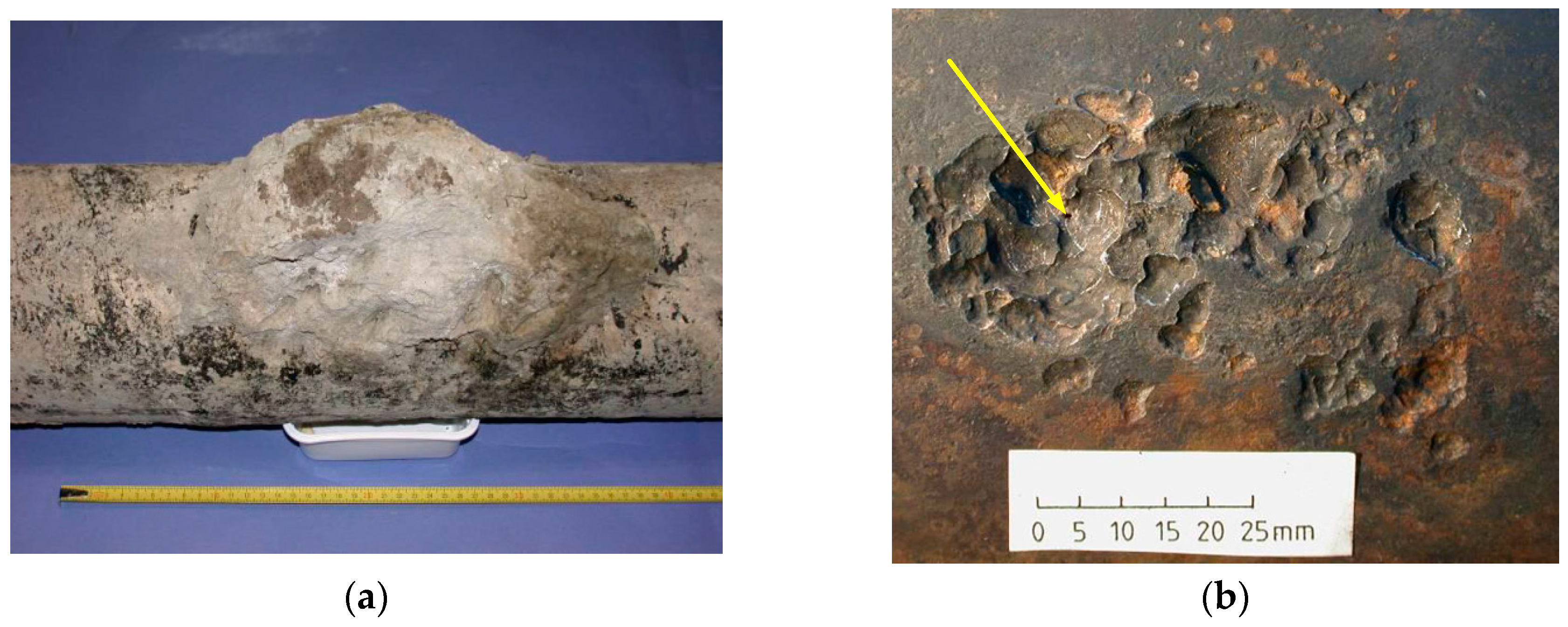
Article

Effects and Characteristics of AC Interference on Parallel Underground Pipelines Caused by an AC Electrified Railway

1
School of Electrical Engineering, Southwest Jiaotong University, Chengdu 611756, China
2
China Petroleum Pipeline Engineering Co., Ltd., Langfang 65000, China
*
Author to whom correspondence should be addressed.
Energies 2018, 11(9), 2255; https://doi.org/10.3390/en11092255
Submission received: 29 July 2018 / Revised: 23 August 2018 / Accepted: 25 August 2018 / Published: 27 August 2018

Abstract

:
An AC electrified railway can interfere significantly with parallel underground pipelines in a public transportation corridor. Such interference may threaten the long-term transportation and the operational safety of the pipelines. Therefore, this paper presents a mathematical model to illustrate the electromagnetic coupling between an AC electrified railway and nearby parallel underground pipelines. As the basis of the engineering calculation, an integration simulation model based on CDEGS software, which included an electrified railway and pipeline system, was built and its correctness was validated by comparing it with a mathematical model. Also, the effects of electric traction load parameters, pipeline parameters, and soil structure parameters were analyzed, the results of which demonstrate the distribution characteristics of AC interference on parallel underground pipelines. Using a real case in China as an example, protection measures were introduced to decrease coupling interference and their effectiveness was verified by simulation calculations and field measurements.

1. Introduction

Due to geographical conditions and cost constraints, electrified railways and oil and gas pipelines are often laid on the same public transport corridor, especially in regions where energy and rail transportation are in great demand. AC interference produced by strong interference sources (i.e., high-voltage AC power supply systems, AC traction system) is a serious issue for nearby underground pipelines. It can result in varying degrees of corrosion on metal structures through electromagnetic coupling and lead to the dangerous for the operating personnel and the equipment connected to it [1]. In the absence of effective protective measures, buried pipelines are severely corroded or even perforated under long-term exposure, endangering transportation and operation safety. According to the measurement results of the Rome–Naples high-speed rail transit line, AC interference is dangerous for the safety of people, in particular, in the case of faults. Further, AC interference can also cause corrosion of buried metallic structures not correctly insulated or protected in a few cases in combination with DC sources [2]. The monitoring data of the pipe potential in a parallel section of power lines, railway lines and the investigated natural gas pipeline in Austria revealed that the inductive influence caused pipeline potential peaks [3]. During a routine inspection of a natural gas transmission line in Canada, it was found that a leak occurred at the end of a pipeline which runs in parallel to a railway (16 2/3-Hz system) for approximately 10 km, as shown in Figure 1 [4].
At present, much of the published literature has focused on AC interference on underground pipelines caused by high-voltage transmission lines in power systems using different methods. Dawalibi [5] used method of moments for calculating the inductive coupling of steady-state AC interference on buried pipelines caused by AC transmission line. Bortels [6] and Christoforidis [7] used the finite element method to calculate the inductive interference caused by HV power lines to nearby buried pipelines under normal operating conditions and fault conditions respectively. Meanwhile, Micu et al. [1] used the finite element method to reveal the influence of the phase shift and the different loading between the two circuits, the unbalanced loading and the phase sequence on the electromagnetic interference between double circuit power lines and nearby pipelines. Tsiamitros et al. [8] used the Hertzian vector method to calculate the complex impedances of a system comprising of overhead and underground insulated conductors in a multilayered earth installation.
However, unlike a three-phase power system, the traction power supply system of a single-phase power frequency (50 Hz) high-voltage power supply system is asymmetrical [9] and uses the rail and the earth as the return path for return current flow back to the supplying traction substations. As such, there is a high stray current, even during normal operation [10]. As the rails and the earth are only insulated by ballast beds or insulating gaskets, the gradual deterioration of insulation performance and the running of high-power electric locomotives (i.e., EMUs) will lead to the increased leakage current of the rails. Therefore, as opposed to steady-state AC interference of power systems caused by inductive coupling [11], the interference of the electrified railway traction power supply system is the instantaneous AC interference under the interaction of inductive coupling and resistive coupling [12,13].
In recent years, with the construction and operation of pipelines and railways, many achievements have been obtained in the research of AC interference on buried pipelines caused by electrified railways. With regard to the actual problem of induced voltages on underground pipelines due to short circuits on overhead lines in the electric traction system, a calculation model was established with EMTP-ATP software [14]. Meanwhile, the joint influence of high-voltage power lines and AC electrified railways on buried pipelines was studied [3]. Further, the effects of the most popular potential mitigation measures along inductively interfered pipelines were given and the pros and cons of the most common potential mitigation measure were discussed [15]. Moreover, with the development of numerical simulation techniques such as boundary element and finite element, the design of AC interference mitigation measures for buried pipelines was carried out by using numerical simulation technology [16,17].
However, the aforementioned studies and many others rarely considers the effects of the complex structure of electrified railway and pipeline, the impact of the parameters of traction load, pipeline, and soil structure on the distribution of AC interference has hardly been discussed or resolved. To this end, this paper aims at providing insight on this problem. The explicit contributions of this paper are listed as follows:
  • A mathematical model of electromagnetic field theory is applied to account for the inductive coupling voltage and resistive coupling voltage on nearby pipelines.
  • A simulation mode including all sections of an AC traction system and nearby pipeline is constructed. This subsequently allows for studying the influence of the above parameters on AC interference.
  • The effects of the traction load position, traction load current, harmonics current, pipeline parameters (i.e., parallel length, parallel interval, coating), and soil resistivity are analyzed, which reveal the distribution of AC interference on the pipeline in the simulation model.
  • Using a real case in China as an example, protection measures were introduced to decrease coupling interference and their effectiveness was verified by simulation calculations and field measurements.

2. Calculation of AC Interference on Parallel Buried Pipelines Caused by Electrified Railway

The traction power supply system uses the rail and the earth as the return path for return current flow back to the supplying traction substations, as shown in Figure 2. In this case, inductive coupling and conductive coupling are the dominant interference mechanisms under a normal AC traction system’s operating conditions [11]. Both of them will produce induced voltage on the pipeline, which will affect the normal operation of the pipeline cathode protection system and age the anticorrosion coating. This might result in the electrochemical corrosion of the pipeline and a threat to human safety. To this end, China’s national standards and industrial standards provide safety limits relevant to AC interference which can be tolerated on steel pipelines. These limits primarily refer to the total acceptable AC interference voltage produced on pipelines by the normal operating conditions of all nearby AC-interfering sources [18,19]. In what follows, the mathematical model for inductive coupling voltage and resistive coupling voltage is presented.

2.1. Calculation of Inductive Coupling Voltage

The induced electromotive force on the pipeline is caused by the contact wire-ground circuit. Meanwhile, the inductive current in opposite directions is generated in the rail-ground circuit by the current in the contact wire-ground circuit, which reduces the induced electromotive force on the pipeline [20], as shown in Figure 3.
During the normal operating state, the induced electromotive force on the metal pipeline caused by the contact and rail-ground circuits is described as follows [20]:
E n = 2 π f M n l I n λ
M n = ( 4.6 lg ( D / d n ) j π / 2 ) × 10 4
D = 0.2085 / f σ × 10 9
where M n is the mutual inductance of contact wire and pipeline, l is the parallel length, d n is the parallel interval, I n is the current in the contact wire, σ is the earth conductivity, D is the equivalent depth of the ground return wire, and λ is the shielding coefficient of the rail; generally, single-track railways take 0.47 and multi-track railways take 0.33.
According to the theory of the transmission line and taking the earth as the reference conductor, the transmission line model of the pipeline-earth electrical circuit is shown in Figure 4 [6].
Based on the configuration given in Figure 4, the corresponding transmission line equations can be formulated as follows:
d U ( x ) d x + Z I ( x ) E ( x ) = 0
d I ( x ) d x + Y U ( x ) = 0
where U ( x ) is the voltage along the pipeline, I ( x ) is the current along the pipeline, Z is the unit length series impedance, Y is the unit length parallel admittance, and E ( x ) is the induction electromotive force of the unit length pipeline.
The induced electromotive force E ( x ) = E is a constant when the transmission line is parallel to the pipeline. In this case, the general solution of U ( x ) can be described as follows:
U ( x ) = A e γ X + B e γ X
I ( x ) = E Z 1 Z C ( A e γ X B e γ X )
where, γ = Z Y is the propagation constant and Z C = Z / Y is the characteristic impedance of the transmission line model of the pipeline-ground electrical circuit.
In practice, the ends of the parallel section of the pipeline are not grounded and the nonparallel sections extend infinitely far away. Therefore, it can be seen that Z 1 = Z 2 = Z C . At the same time, U ( 0 ) = Z 1 ( 0 ) and U ( L ) = Z 2 I ( l ) are known from the constraint conditions of the end of the transmission line model.
According to the Equations (4) and (5), it can be further derived as:
A = E 2 γ , B = E 2 γ
Therefore, the inductive voltages of each point along the pipeline can be obtained:
U ( x ) = E 2 γ ( e γ ( x l ) e γ x )

2.2. Calculation of Resistive Coupling Voltage

A schematic diagram of the calculation of resistive coupling voltage on a parallel underground pipeline is presented in Figure 5.
As shown in Figure 5, the traction load current leakage point is the coordinate origin. N ( x , y ) is a point on the parallel underground pipeline I g is the current in the rail.
When the traction load current I injects into the rail, the current in the rail I g is:
I g = { I 2 e γ p x ( x > 0 ) I ( x = 0 ) I 2 e γ p x ( x < 0 )
where γ p is the propagation constant of the rail-ground circuit, x is the horizontal distance from point N to the leakage point, and y is the vertical distance from point N to the leakage point.
The current d I g flows into the earth through resistive coupling. Therefore, an electric potential will form at any point N (as shown in Figure 6a) on the buried pipeline, which can be determined from the potential of point M (as shown in Figure 6b) according to the equivalent circuit of the pipeline on the ground.
The electric potential of point N on the buried pipeline can be formulated as follows:
V N = V M = ρ γ d I g 2 π Ω ( γ x 1 , γ y 1 )
Ω ( u , v ) = 1 2 [ e u f ( γ x 1 , γ y 1 ) + e u f ( γ x 1 , γ y 1 ) ]
f ( γ x 1 , γ y 1 ) = u e γ ( x x 1 ) [ γ ( x x 1 ) ] 2 + ( γ y 1 ) 2 d τ
Ignoring the reverse reaction and the mutual impedance between the pipeline-ground and rail–ground circuits, the potential between pipeline and ground at point N on the pipeline can be obtained from Equations (10) and (11):
V N = ρ γ 2 γ p 2 I λ 2 π ( γ p 2 γ 2 ) [ 1 γ Ω ( γ x , γ y ) 1 γ p Ω ( γ p x , γ p y ) ]
where I is the current of the locomotive injected into the rail, γ is the propagation coefficient of the pipeline-ground circuit, γ p is the propagation coefficient of the rail–ground circuit, ρ is the soil resistivity, and λ is the shielding coefficient of the rail.
From Equations (9) and (14), it can be seen that the distribution of AC interference on buried pipelines is affected not only by the traction load current but also by the propagation constant of the pipeline-earth and rail–earth circuits, which are determined by the electrical topology and parameters of the traction power supply system, the parameters of the pipeline, and the soil structure.

3. Simulation Model for AC Interference on Parallel Buried Pipelines Caused by Electrified Railways

3.1. Simulation Model

This study used the direct power supply mode with a return line as an example. The simulation model for AC interference on parallel buried pipelines caused by an electrified railway was formulated in the HiFREQ module of the CDEGS software. For AC interference studies, the advantage of HIFREQ is concurrent calculation of inductive and conductive couplings. Through the HiFREQ model, calculation of the distribution of current, electric field, magnetic field and electric potential (including conductor and coating potential) in the space above ground and underground can be performed from 0 Hz to several tens of MHz for model inside an infinite medium or in a multi-layered soil medium. The simulation model formulated is illustrated in Figure 7.

3.1.1. Modeling of the Traction Substation

The traction transformer was constructed by the single-phase transformer provided by the HiFREQ module. The parameters of the transformer simulation are shown in Table 1.
The X-Z plan view of the traction substation grounding grid is shown in Figure 8. The earthing impedance of the grounding grid was 0.3 Ω.
The parameters of the grounding grid are shown in Table 2.

3.1.2. Modeling of Catenary

Taking the direct power supply with return wires as an example, the topological arrangement of a single-phase AC traction supply and supporting system is shown in Figure 9.
The type of messenger wire was JTMH95. The type of contact wire was CTMH120. The type of return wire was LBGLJ-185/10. The type of boosting cable was YJV-150 and the setting interval was 1.5 km [21].

3.1.3. Modeling of Rails

P60 railway standard rails were selected according to TB/T3276-2011 [22]. The parameters are shown in Table 3:

3.1.4. Modeling of Underground Pipeline

The buried pipeline was a steel pipe and the anticorrosion coating was a three-layer polyethylene (3PE) coating. The parameters are shown in Table 4.

3.2. Validation of Impedance Characteristics of the Traction Power Supply Circuit

The traction power supply system simulation model determines the load flow distribution of the power supply network, and it is also an important basis for the assessment of resistively coupling AC interference on buried pipelines. Further, the short circuit impedance characteristics of the traction supply circuit can be used to describe the accuracy of the simulation model. A comparison between the results of the simulation model and the Carson theory is shown in Table 5.
From Table 5, it can be seen that there is very good agreement between the simulation and the Carson theory results. Furthermore, as the distance increases, the error decreases and does not go exceed 5%. The main reason for the error is that the Carson theory only considers the traction network impedance and ignores the grounding resistance effect on the short circuit impedance. The simulation model based on CDEGS software adds a grounding grid model in the traction substation, and the impact is obvious when the short circuit point is close to the traction substation.

3.3. Characteristic Analysis of Inductive Coupling and Resistive Coupling

Using the mathematical model and simulation model to calculate the inductive coupling voltage and the resistive coupling voltage, the effect of the horizontal distance between the electrified railway and the pipeline on the AC interference voltage distribution of the pipeline can be evaluated. A comparison between the simulation and calculation results is given in Table 6.
From Table 6, it can be seen that the simulation results are basically the same as the calculation results. The error decreases with the increase of horizontal distance between the parallel buried pipeline and the center point of the pipeline. This is because as the horizontal distance decreases, the magnetic shielding effect of the rail becomes stronger. Therefore, the simulation model based on CDEGS software has a high calculation accuracy and can be used to simulate the electromagnetic coupling effect of a traction power supply system on the distribution of AC interference on buried pipelines.

4. Simulation Analysis of Influence Factors

The further particulars of the simulation model are as follows: the length of the power supply arm of the traction power supply system was 20 km; the parallel length between the buried pipeline and the railway was 5 km; the parallel interval was 250 m; the soil resistivity of the public transmission area was 100 Ω · m ; the traction load location was 10 km; and the traction load current was 500 A. The relative positions between the electrified railway and the buried pipeline is shown in Figure 10.

4.1. Traction Load Parameters

4.1.1. Traction Load Current

Five kinds of typical operating conditions (200, 400, 600, 800 and 1000 A) were selected as the traction load currents. The distribution of the AC interference voltage on the buried pipeline at different traction load currents is presented in Figure 11.
As the traction load current increases, the AC interference voltage on the pipeline increases. Taking the currents of 200 A and 800 A as examples, the maximum AC interference voltages of the pipeline are 10.04 V and 52.51 V, respectively, and the voltage increases 4.23 times. This is due to the increase of traction load current which causes the leakage current increases, and therefore, it leads to the AC interference voltage rise on the pipeline. The relationship between the extreme value of the AC interference voltage on the pipeline and the traction load current when the traction load current is different is presented in Figure 12.
It can be seen that the extremes of the pipeline AC interference voltage (maximum 1, maximum 2 and minimum) increase with the increasing traction load current. The growth rate of maximum 1 (AC interference voltage at the end point of the pipeline, which is close to the substation) is larger than that of maximum 2 (AC interference voltage at the end point of the pipeline, which is far away from the substation), and the maximum growth rate is much higher than the minimum.

4.1.2. The Position of the Traction Load

Four kinds of typical operating conditions (5 km, 10 km, 15 km and 20 km) were selected as the distances between the train and traction substation. The distribution of the AC interference voltage on the buried pipeline at different distances between the traction load and traction substation is presented in Figure 13.
With the traction load away from the traction substation, the magnitude of the AC interference voltage on the pipeline will increase. When the traction load is located at 5 km and 20 km, the maximum AC interference voltage of the pipeline is 2.45 V and 38.77 V, respectively, and the voltage increases 14.8 times. This is because the traction power supply system uses the rail and the earth as the return path for return current, with the traction load away from the traction substation, the impedance of rail return path will increase. This will lead to the increase of return current in the earth return path and therefore it results in the AC interference voltage rise on the pipeline.
The relationship between the AC interference voltage distribution and traction load position at different points on the pipeline when the traction load is in a different position is presented in Figure 14.
It can be seen that the AC interference voltage of the pipeline increases with the increase of the distance between the traction load and traction substation. When the distance is beyond about 15 km, the AC interference voltage tends to be stable and reaches the maximum value. When the traction load runs throughout the power supply arm, the AC interference voltage along the pipeline is symmetrical at about the center point of the pipeline. The maximum value of the AC interference voltage at the two symmetrical positions is basically the same, and the growth trend is also basically in agreement.

4.1.3. Harmonics

Harmonics are a common problem for electrified railways [23]. The AC-DC electric locomotive harmonics are mainly third, fifth, seventh, and so on [24]. In this model, four typical operating conditions (third, fifth, seventh and ninth harmonics) were selected. The harmonic current data are shown in Table 7.
The distribution of the AC interference voltage on the buried pipeline at different harmonic currents is presented in Figure 15.
The maximum AC interference voltages of the third, fifth, seventh, and ninth harmonics are 19.9 V, 8.96 V, 6.71 V and 10.7 V, respectively. It can be seen that the AC interference voltages caused by low-order harmonic currents are still beyond the AC interference voltage limit of 4 V, which was specified in the national standard GB/T50698-2011 [19].

4.2. Parallel Pipeline Parameters

4.2.1. Parallel Length

According to the principle of electromagnetic coupling, when the pipeline is parallel to the electrified railway, the parallel length and parallel interval between the pipeline and railway have a significant impact on the distribution of AC interference voltages on pipelines. Five kinds of typical operating conditions (2, 4, 6, 8 and 10 km) were selected as the parallel lengths of pipeline. The distribution of the AC interference voltage on the buried pipeline at different parallel lengths is presented in Figure 16.
As the parallel length increases, the AC interference voltage on the pipeline increases. Taking the pipeline parallel lengths of 2 km and 10 km as examples, the maximum AC interference voltages of the pipeline are 10.65 V and 54.37 V, respectively, and the voltage increases 4.1 times. It is obviously that the minimum voltage is observed at the center point. This is due to the minimum leakage current is at this point. Moreover, the maximum voltage occurs at the two end points of the pipeline. This is because as the parallel length increases, the induced electromotive increases, and thus it results in a large AC interference voltage at the two end points. Meanwhile, it also causes the increase of AC interference voltage on the pipeline with the l parallel length increases.
The relationship between the distribution of the extreme voltages (maximum 1, maximum 2 and minimum) and the parallel length of the pipeline AC interference voltage when the parallel length of the pipeline is different is presented in Figure 17.
It can be seen that the extreme values of the pipeline AC interference voltages (maximum 1, maximum 2 and minimum) increase with the increase of the parallel length. The growth rate of maximum 1 (AC interference voltage at the end point of the pipeline, which is close to the substation) is larger than that of maximum 2 (AC interference voltage at the end point of the pipeline, which is far away from the substation), and the maximum growth rate is much higher than the minimum.

4.2.2. Parallel Interval

Five kinds of typical operating conditions (200 m, 400 m, 600 m, 800 m and 1000 m) were selected as the parallel intervals of the pipeline. The distribution of the AC interference voltage on the buried pipeline at different parallel intervals is presented in Figure 18.
As the parallel interval increases, the AC interference voltage on the pipeline decreases. Taking the pipeline parallel intervals of 200 m and 1000 m as examples, the maximum AC interference voltages of the pipeline are 15.39 V and 3.42 V, respectively, and the voltage drops by 77.8%. This is because as the parallel interval increases, the induced electromotive decreases, and therefore it results in the decrease of AC interference voltage on the pipeline.
The relationship between the distribution of the extreme voltages (maximum 1, maximum 2 and minimum) and the parallel separation distance of the pipeline AC interference voltage when the parallel interval of the pipelines is different is presented in Figure 19.
It can be seen that the extreme values of the pipeline AC interference voltage (maximum 1, maximum 2 and minimum) decrease with the increase of the parallel interval, and the reduction rate of the extreme values decreases with the increase of the parallel interval distance. The reduction rate of maximum 1 (AC interference voltage at the end point of the pipeline, which is close to the substation) is larger than that of maximum 2 (AC interference voltage at the end point of the pipeline, which is far away from the substation), and the maximum reduction rate is much higher than the minimum.

4.2.3. Anticorrosion Coating of Pipelines

Anticorrosion coatings have been widely utilized on pipelines to protect the steel structures from environmental attack. This is done to avoid the loss of cathode current and to prevent corrosion of the pipe. The coating resistance is a significant parameter that reflects performance. The anticorrosion coating materials are mainly divided into asphalt (10,000 Ω · m 2 ), epoxy powder (30,000 Ω · m 2 ), and 3 PE coatings (100,000 Ω · m 2 ). These three kinds of typical conditions (asphalt, epoxy powder and 3 PE coatings) were selected as the pipeline coatings. The distribution of AC interference voltages on buried pipelines with different coatings is presented in Figure 20.
As the resistance of the pipeline coating increases, the AC interference voltage of the pipeline increases. Taking asphalt, epoxy powder and 3 PE coatings as examples, the maximum AC interference voltages in the pipeline are 12.97, 18.09 and 21.13 V, respectively. This is because the increase of pipeline coating resistance blocks the exchange of current between the pipeline and the earth. It forces a large induced current on the pipeline and causes the AC interference voltage rise on the pipeline.
The relationship between the distribution of the extreme values of the AC interference voltage (maximum 1, maximum 2, and minimum) and the resistance of the coating when the resistance of the pipeline coating is different is presented in Figure 21.
It can be seen that as the resistance of the coating increases, the maximum value of the AC interference voltage (maximum 1, maximum 2) increases, and the growth rates of maximum 1 and maximum 2 are basically the same. The growth rate of the maximum value decreases with the increase of the resistance. Once the resistance of the coating goes beyond about 90,000 Ω · m 2 , the AC interference voltage tends to be stable. However, the resistance has no appreciable influence on the minimum value.

4.3. Soil Parameters

Five kinds of typical operating conditions (200, 400, 600, 800 and 1000 Ω · m ) were selected as the soil resistances. The distribution of the AC interference voltages on the buried pipeline at different soil resistances is presented in Figure 22.
As the soil resistance increases, the AC interference voltage of the pipeline increases. Taking the soil resistances of 200 and 1000 Ω · m as examples, the maximum AC interference voltages of the pipeline are 30.81 and 48.78 V, respectively, and the voltage increases by 58.33%. This is because as the soil resistance increases, the pipeline resistivity decreases relatively. It concentrates the current on the pipe, causing the AC interference voltage to rise on the pipeline.
The relationship between the distribution of the extreme values of the AC interference voltage (maximum 1, maximum 2 and minimum) and the soil resistance when the soil resistance is different is presented in Figure 23.
The maximum 1 (AC interference voltage at the end point of the pipeline, which is close to the substation) and the minimum increase with the increase of soil resistance, and the growth rate of maximum 1 is larger than the minimum. However, the soil resistance has no appreciable influence on maximum 2 (AC interference voltage at the end point of the pipeline, which is far away from the substation).

5. Field Measurements and Case Study

In this paper, the AC interference between the Baotou–Lanzhou railway and Lanzhou–Yinchuan gas pipeline was investigated and studied. The positional relationship between the railway and pipeline is presented in Figure 24.
The length of the Baiyin branch line of Lanzhou Yinchuan gas pipeline is 54 km, the size of the pipeline is ϕ273 × 10 mm, and it has a 3PE external anticorrosion coating and forced current cathode protection. The pipelines are laid parallel or cross to the Baolan electrified railway in the section between the test piles of JP45-JP55. The parameters of each test point are shown in Table 8.
The power supply system of the west section of the Baiyin railway is a direct power supply with return wires. The electrical diagram of the substation is shown in Figure 25. It is a typical structure diagram of traction substation for 27.5 kV AC electrified railway, which is also the basis of the traction substation modeling based on HiFREQ module of the CDEGS software. The length of the power supply arm of the Zhujiayao feeder is 13.73 km. The length of the power supply arm of the Doujiagou feeder is 14.32 km. The impedance of the traction network is 6.71 Ω. Furthermore, the location of the field measurement is labeled by the red dots in Figure 25, which can provide more details for easy understanding in the case study. The traction load currents were measured by the Zhujiayao feeder and Dujiagou feeder. The ground return current and rail return current were measured by the ground return line and ground line of transformer 1#B and 2#B. These data can be used for optimization design of the protection measures below.
The parameters of the traction transformer are shown in Table 9.
The simulation model of AC interference on parallel buried pipelines caused by an electrified railway was constructed based on the relevant structural parameters of the Baiyin West traction substation and Baiyin branch pipeline (traction transformer, grounding grid, traction network, pipeline, coating, line GPS coordinates, etc.), traction load test data and the soil resistivity of the common transmission corridor.

5.1. Simulation of Return Current

Based on the test data and simulation results of the traction substation, the distribution characteristics of the traction return current (rail return current and ground return current) of the Baiyin traction substation were obtained. Taking the largest traction load current during the field measurement as an example (350 A Harmony (HX) electric locomotive), the results of the distribution of the traction return current are shown in Figure 26.
The error of each traction return current (rail return current and ground return current) of the traction substation was less than 8%. When the locomotive was located at the test pile No. 55 (measuring point 1), which is close to the traction substation and the high-voltage transmission line, the error was the largest. However, the errors of the rail return current and ground return current were only 7.72% and 6.08%, respectively.

5.2. Simulation of Undraining Condition

Based on the measurement data of traction load current and AC interference voltage, the fitting result of the distribution of AC interference on the pipeline without applying the drainage was obtained. Taking the largest traction load current during the field measurement as an example (350 A Harmony (HX) electric locomotive), the results of the distribution of AC interference voltages on the pipeline are shown in Figure 27 and Figure 28.
The error of the AC interference voltage is less than 1 V, and the fitting accuracy of the AC interference voltage at different measurement points is satisfied. Comparing the AC interference voltage of the cross and parallel sections, it can be seen that both of them are beyond the AC interference voltage limit of 4 V specified in the national standard GB/T50698-2011 [19]. Also, the AC interference density index J AC (the soil resistivity of the test section is 53 Ω · m ) was calculated according to the standard, and the AC interference level was “middle”, so AC interference protection measures should be taken in this section.

5.3. Simulation of Draining Condition

The field measurements and simulation analysis showed that there was serious AC interference on the pipeline. Combined with the Baiyin branch line and construction conditions, drainage devices were installed for the pipelines in the interference section. In Table 10, the test piles with drain conductor installed are listed and the real grounding resistance values taken from field measurements of the drainage devices are shown.
The grounding electrode of the drainage device is steel pipe (ϕ50 × 5) which is buried vertically, as shown in Figure 29.
Combined with the measurement data of traction load current and the AC interference voltage on the pipeline, the fitting results of the real distribution and simulation of the AC interference voltage under the draining condition were obtained. Taking the largest traction load current during the field measurement as an example (350 A Harmony (HX) electric locomotive), the results of the distribution of AC interference voltages on the pipeline are shown in Figure 30 and Figure 31.
The error of pipeline AC interference voltage is less than 0.4 V, and the fitting accuracy of the AC interference voltage at different measurement points is satisfied. The AC interference voltage on the pipeline in the cross and parallel sections drops below to 4 V, which satisfies the requirement of the national standard. The maximum value of the AC interference density index J AC is 15.61 A/m2, which satisfies the drainage requirement limit of 60 A/m2.
The protection measures proposed above reduces the voltage on the pipeline and avoids corrosion caused by AC interference. As a compromise between technical and economic factors on different projects, the iterative optimization of the protection measures should be performed to provide a better protection effect.

6. Conclusions

This paper studies the inductive coupling voltage and resistive coupling voltage on buried pipelines caused by an AC traction power supply system. This was accomplished by building a mathematical model based on the inductive coupling and resistive coupling theory and a simulation model based on CDEGS software, which include an electrified railway and pipeline system. The correctness of mathematical model and simulation model has been validated by mutual comparison.
In simulation model, the effects and sensitivity of traction load parameters, parallel pipeline parameters and soil parameters on the AC interference voltage on pipeline have been discussed. Among the above factors, the traction load current, the traction load position, and the parallel length of the pipeline have a significant influence on the interference voltage which should be considered as a key point when designing electrified railways and oil and gas pipelines to avoid excessively high AC interference voltage on the pipeline. Meanwhile, in most simulation results, the AC interference voltages on the pipeline are beyond the limit of 4 V, which was specified in the national standard. Therefore, it is necessary to implement protection measures for pipelines. Using a real case in China as an example, protection measures were introduced to decrease coupling interference and their effectiveness was verified by simulation calculations and field measurements. In conclusion, the outcomes of this paper can provide engineering guidance for the design and protection of railways and pipelines.

Author Contributions

J.Z. and M.C. proposed the idea. S.L. and J.Z. developed the model, performed the simulation works and wrote the paper. S.L., C.X., H.T. were in charge of review and editing. This work was conducted under the supervision of M.C. and J.L.

Funding

This research was funded by the National Natural Science Foundation of China (Grant No. 51877182) and the Science and Technology Plan Project of Sichuan Province (Grant No. 2018FZ0107). APC was funded by the National Natural Science Foundation of China and the Science and Technology Plan Project of Sichuan Province.

Acknowledgments

This research was supported by China Petroleum Pipeline Engineering Co., Ltd. (CPP) and the First Design and Survey Institute (FDSI) Group Co., Ltd.

Conflicts of Interest

The authors declare no conflict of interest.

References

  1. Micu, D.D.; Christoforidis, G.C.; Czumbil, L. AC interference on pipelines due to double circuit power lines: A detailed study. Electr. Power Syst. Res. 2013, 103, 1–8. [Google Scholar] [CrossRef]
  2. Santi, G.; Sandrolini, L. Stray current interferences on high-speed rail transit systems and surrounding buried metallic structures. In Proceedings of the 6th International Congress CEOCOR, Giardini Naxos, Messina, Italy, 13–16 May 2003; pp. 1–12. [Google Scholar]
  3. Fickert, L.; Schmautzer, E.; Braunstein, R.; Lindinger, M. Reduction of the electrical potential of interfered pipelines due to currents of high voltage power lines and electric railways. E I Elektrotech. Inf. 2010, 127, 362–366. [Google Scholar] [CrossRef]
  4. Linhardt, P.; Ball, G. AC Corrosion: Results from Laboratory Investigations and from a Failure Analysis. In CORROSION/2006; NACE International: Houston, TX, USA, 2006; pp. 061601–061609. [Google Scholar]
  5. Dawalibi, F.P. Electromagnetic field generated by overhead and buried short conductor, part 1: Single conductor. IEEE Trans. Power Deliv. 1986, 1, 105–111. [Google Scholar] [CrossRef]
  6. Bortels, L.; Deconinck, J.; Munteanu, C.; Topa, V. A general applicable model for ac predictive and mitigation techniques for pipeline networks influenced by HV power lines. IEEE Trans. Power Deliv. 2006, 21, 210–217. [Google Scholar] [CrossRef]
  7. Christoforidis, G.C.; Labridis, D.P.; Dokopoulos, P.S. A hybrid method for calculating the inductive interference caused by faulted power lines to nearby buried pipelines. IEEE Trans. Power Deliv. 2005, 20, 1465–1473. [Google Scholar] [CrossRef]
  8. Tsiamitros, D.A.; Christoforidis, G.C.; Papagiannis, G.K.; Labridis, D.P.; Dokopoulos, P.S. Earth conduction effects in systems of overhead and underground conductors in multilayered soils. IEE Proc.-Gener. Transm. Distrib. 2006, 153, 291–299. [Google Scholar] [CrossRef]
  9. Matta, V.; Kumar, G. Unbalance and voltage fluctuation study on ac traction system. In Proceedings of the 2014 Electric Power Quality and Supply Reliability Conference (PQ), Rakvere, Estonia, 11–13 June 2014; pp. 303–308. [Google Scholar]
  10. Mariscotti, A. Distribution of the traction return current in ac and dc electric railway systems. IEEE Trans. Power Deliv. 2003, 18, 1422–1432. [Google Scholar] [CrossRef]
  11. Czumbil, L.; Micu, D.D.; Stet, D.; Ceclan, A. A neural network approach for the inductive coupling between overhead power lines and nearby metallic pipelines. In Proceedings of the 2016 International Symposium on Fundamentals of Electrical Engineering (ISFEE), Bucharest, Romania, 30 June–2 July 2016. [Google Scholar]
  12. Charalambous, C.A.; Demetriou, A.; Lazari, A. Effects of Electromagnetic Interference on Underground Pipelines caused by the Operation of High Voltage A.C. Traction Systems: The Impact of Harmonics. IEEE Trans. Power Deliv. 2018, 99, 1. [Google Scholar] [CrossRef]
  13. EN 15280:2013. Evaluation of a.c. Corrosion Likelihood of Buried Pipelines Applicable to Cathodically Protected Pipeline; EN: Brussels, Belgium, 2013. [Google Scholar]
  14. Milesevic, B.; Filipovic-Grcic, B.; Radosevic, T. Electromagnetic fields and induced voltages on underground pipeline in the vicinity of ac traction system. J. Energy Power Eng. 2014, 8, 1333–1340. [Google Scholar]
  15. Braunstein, R.; Schmautzer, E.; Graz, G.P. Comparison and discussion on potential mitigating measures regarding inductive interference of metallic pipelines. In Proceedings of the Electrical Systems for Aircraft, Railway and Ship Propulsion, Bologna, Italy, 19–21 October 2010. [Google Scholar]
  16. Zhao, J.; Shen, G.J.; Yin, X.D.; Chen, Z.H.; Xue, Z.Y.; Chen, H.Y. Using Computer Software to Simulate AC Interference and Mitigation Measures of Buried Pipelines. In ICPTT 2012: Better Pipeline Infrastructure for a Better Life; ASCE: Reston, VA, USA, 2012; pp. 161–170. [Google Scholar]
  17. Du, Y.X.; Jiang, Z.T.; Lu, M.X. Study on AC Interference Mitigation Design Methods for Buried Pipelines. In CORROSION/2013; NACE International: Houston, TX, USA, 2013. [Google Scholar]
  18. SY/T0032-2000: Standard for AC Influence Drainage Protection of Buried Steel Pipeline; China Petroleum and Chemical Industry Federation: Beijing, China, 2000.
  19. GB/T50698-2011: Standard for AC Interference Mitigation of Buried Steel Pipelines; Ministry of Housing and Urban-Rural Development: Beijing, China, 2011.
  20. Wang, W.J.; Li, Q.Z.; Zhang, L. The Computation of the Induction Voltage Based on the System of Two Transmission Lines over One Rail. High Volt. Eng. 2003, 29, 22–23. [Google Scholar]
  21. TB 10621-2014: Code for Design of High Speed Railway; China Railway: Beijing, China, 2014.
  22. TB/T3276-2011: Rails for High Speed Railway; China Railway: Beijing, China, 2011.
  23. He, X.Q.; Guo, A.P.; Peng, X.; Zhou, Y.Y.; Shi, Z.H.; Shu, Z.L. A traction three-phase to single-phase cascade converter substation in an advanced traction power supply system. Energies 2015, 8, 9915–9929. [Google Scholar] [CrossRef]
  24. Wang, J.H.; Zhang, M.; Li, S.W.; Zhou, T.D.; Ou, H.J. Passive filter design with considering characteristic harmonics and harmonic resonance of electrified railway. In Proceedings of the 2017 8th International Conference on Mechanical and Intelligent Manufacturing Technologies (ICMIMT), Cape Town, South Africa, 3–6 February 2017; pp. 174–178. [Google Scholar]
Figure 1. Leak site on underground natural gas transmission pipeline (attributed to AC corrosion). (a) Before cleaning; (b) After cleaning. The arrow indicates the leak.
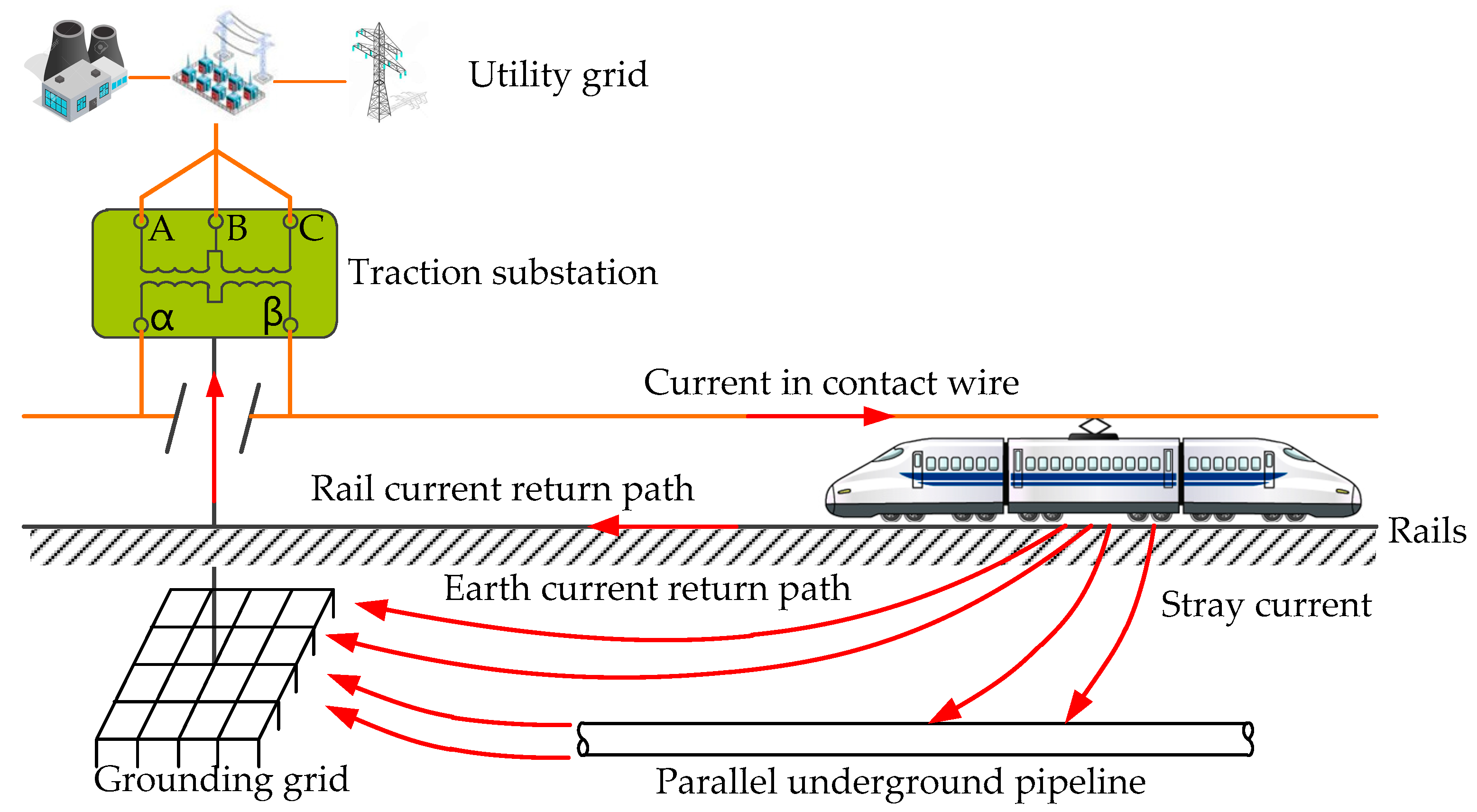
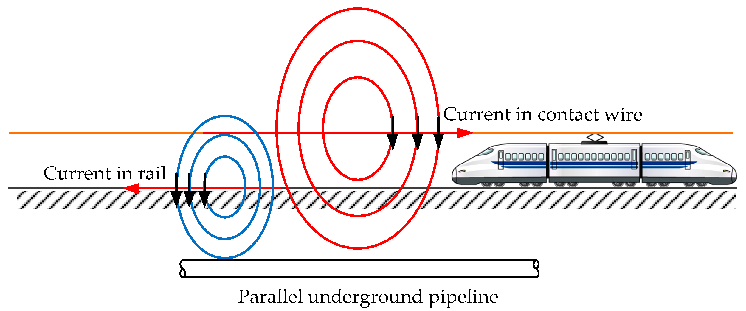
Energies 11 02255 g001
Figure 2. AC interference on a parallel underground pipeline caused by electrified railway.
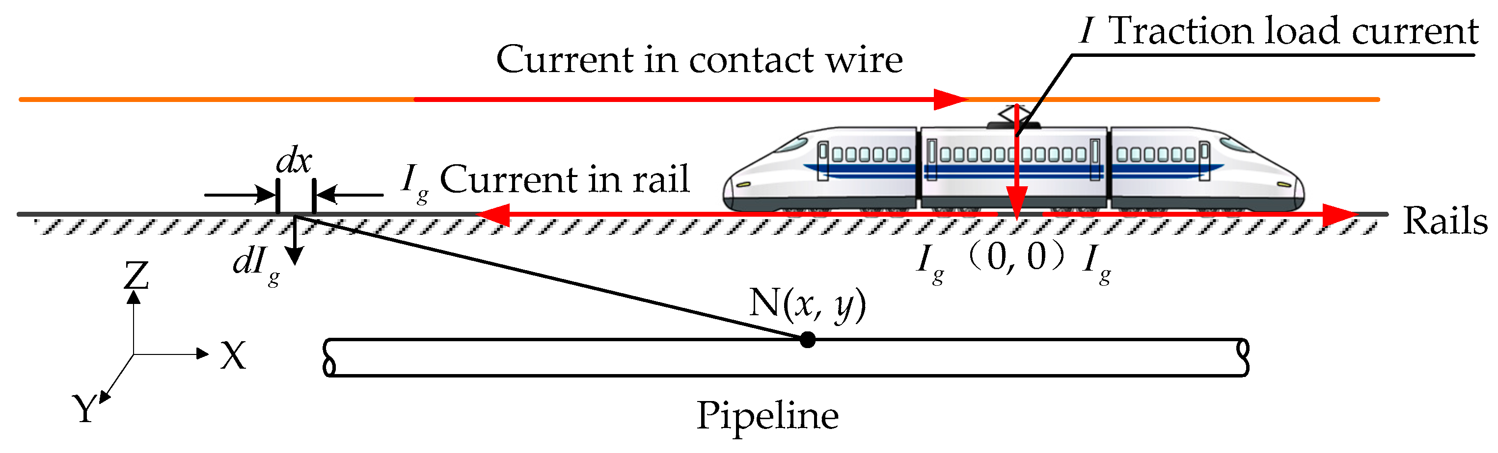
Energies 11 02255 g002
Figure 3. Calculation of inductive voltage on a parallel pipeline.
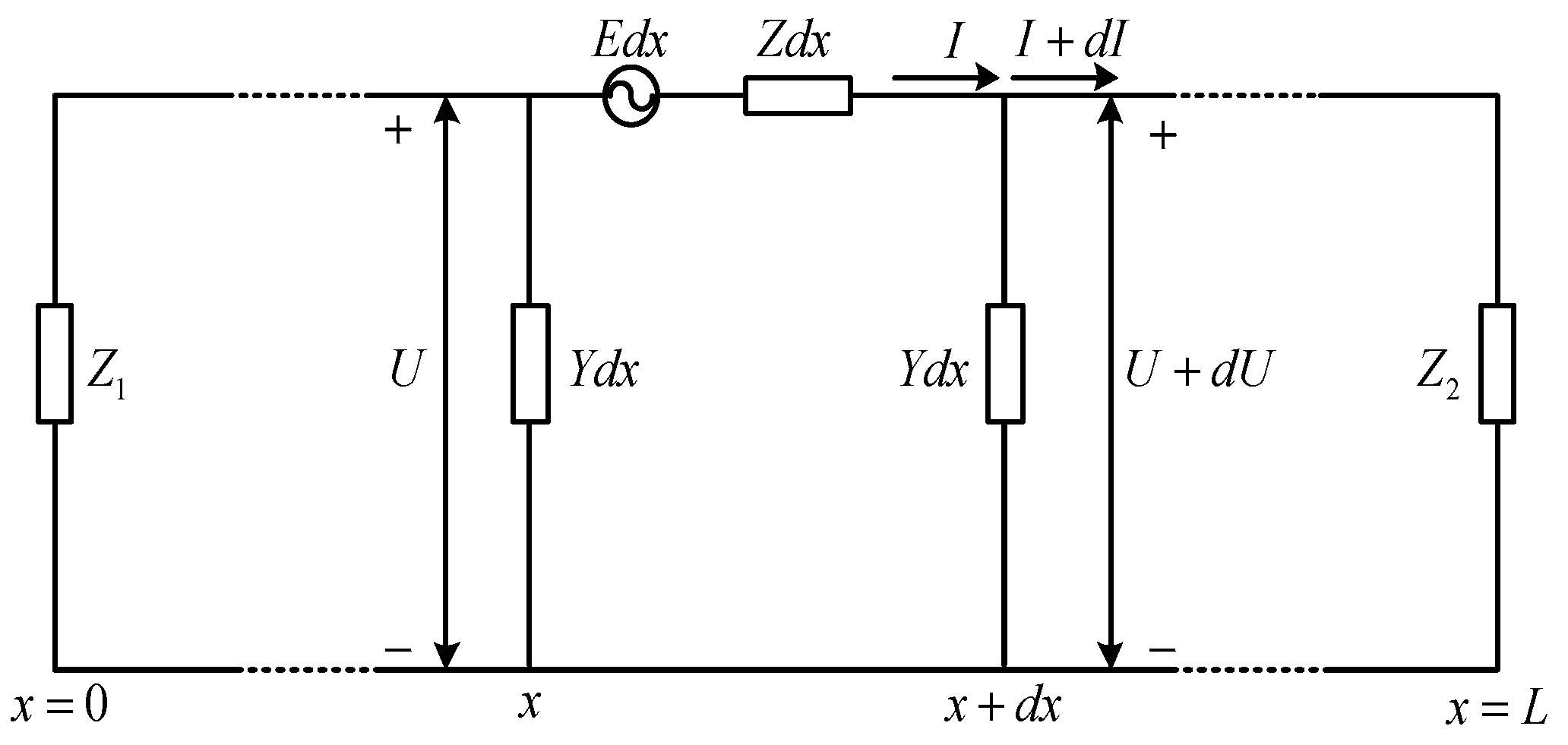
Energies 11 02255 g003
Figure 4. Transmission line model of the pipeline-ground electrical circuit.
Energies 11 02255 g004
Figure 5. Calculation of resistive voltage on a parallel pipeline.
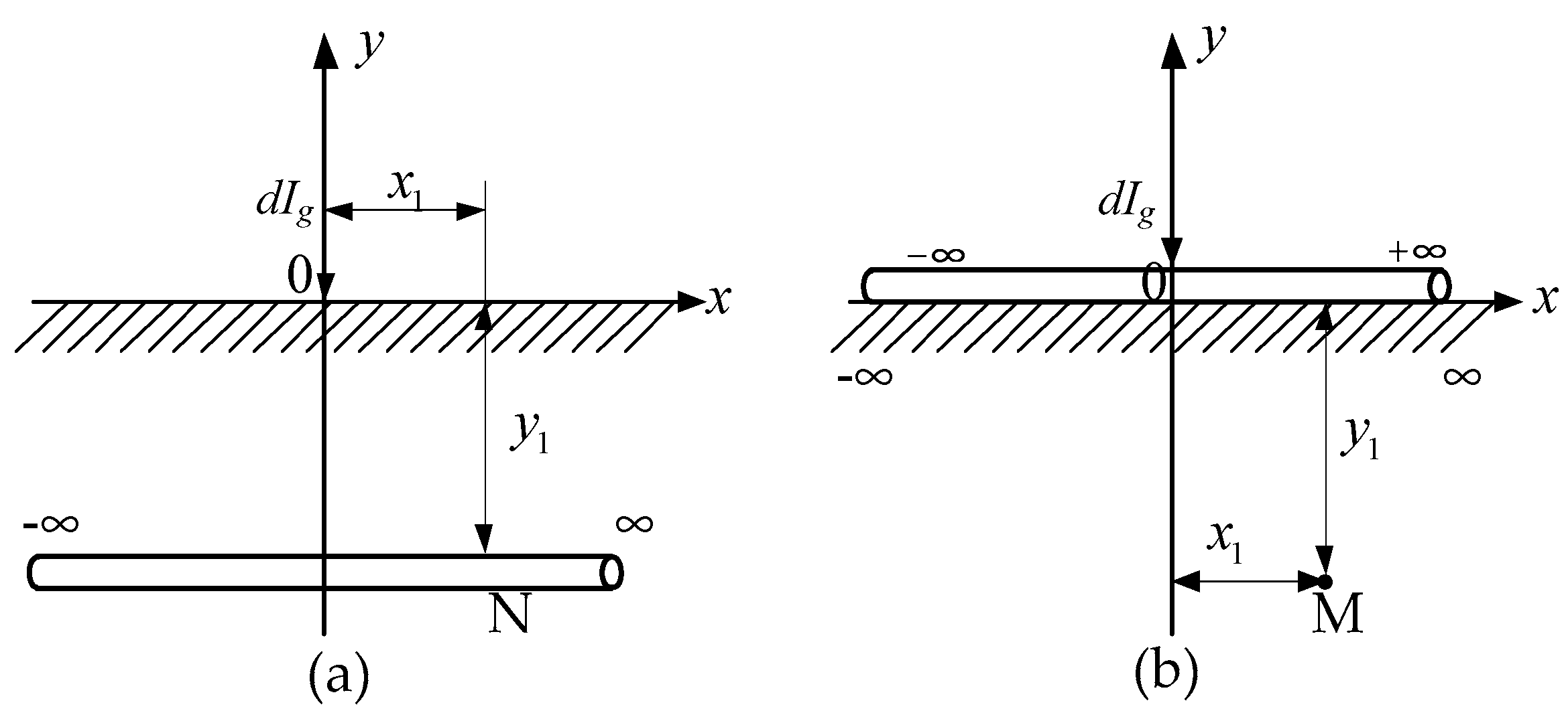
Energies 11 02255 g005
Figure 6. Interference on a parallel buried pipeline caused by ground current. (a) The electric potential at point N on the buried pipeline; (b) The electric potential on point M caused by leakage current from ground pipeline.
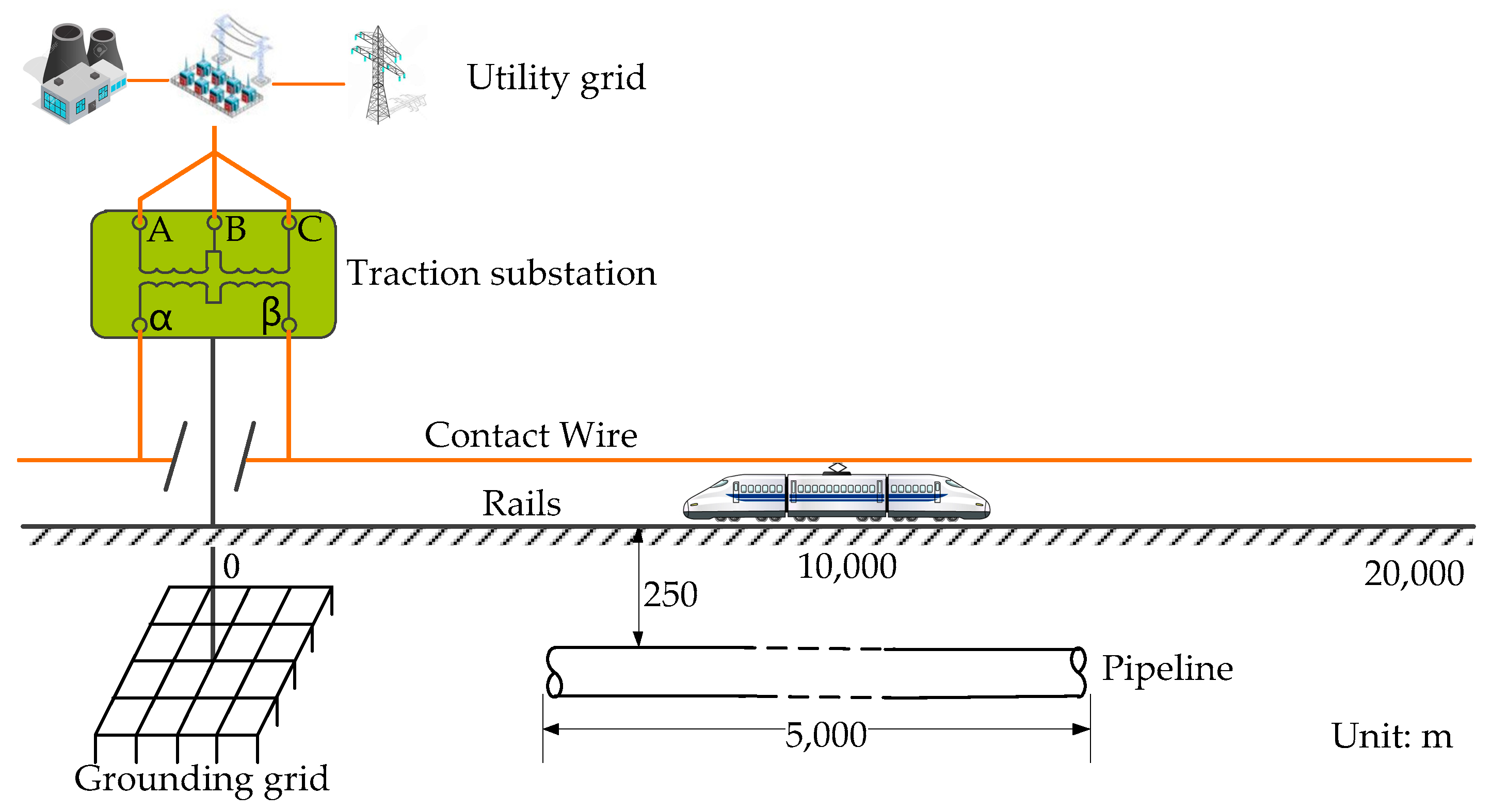
Energies 11 02255 g006
Figure 7. Model for AC interference on parallel buried pipelines caused by an electrified railway.
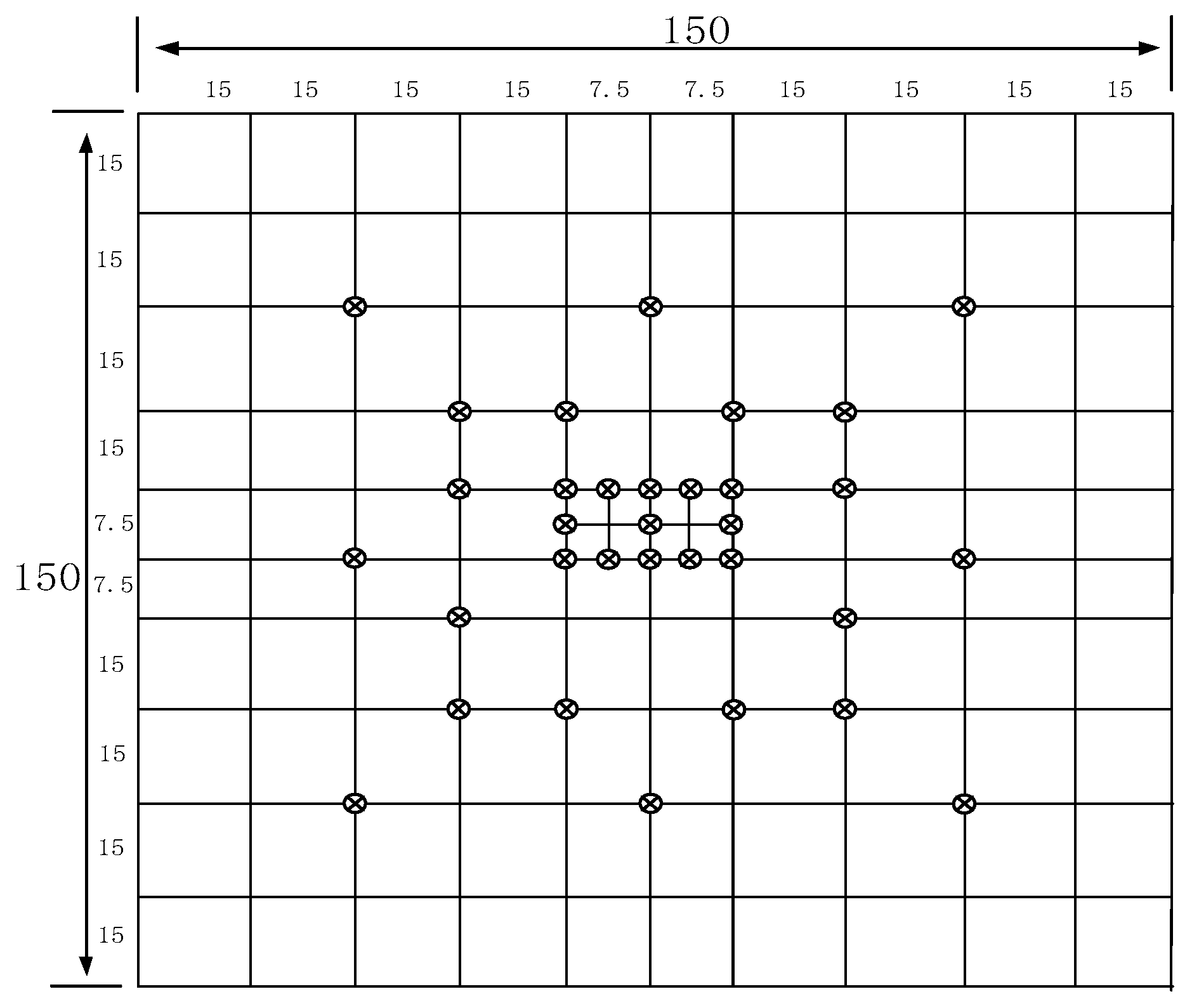
Energies 11 02255 g007
Figure 8. X-Z plan view of the grounding grid.
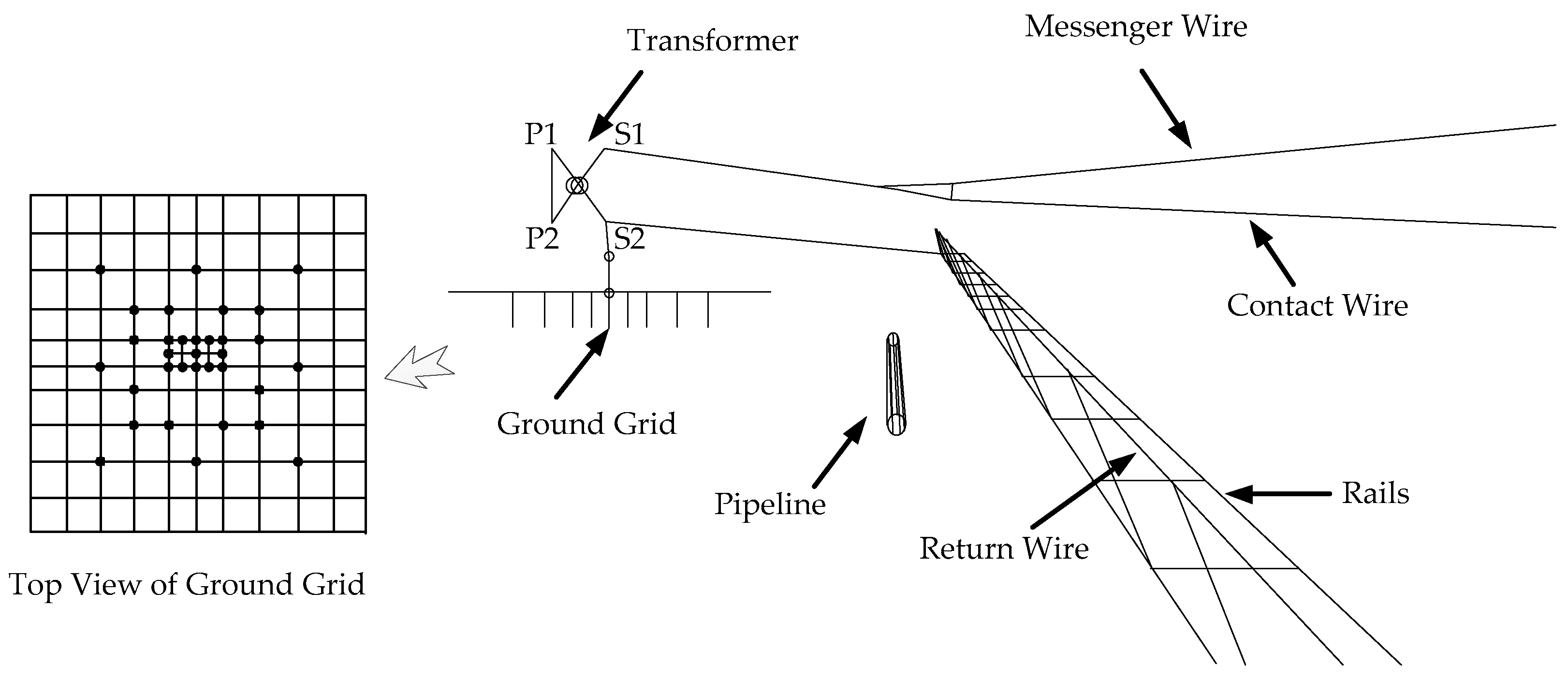
Energies 11 02255 g008
Figure 9. Topological arrangement of a single-phase AC traction supply and supporting system.
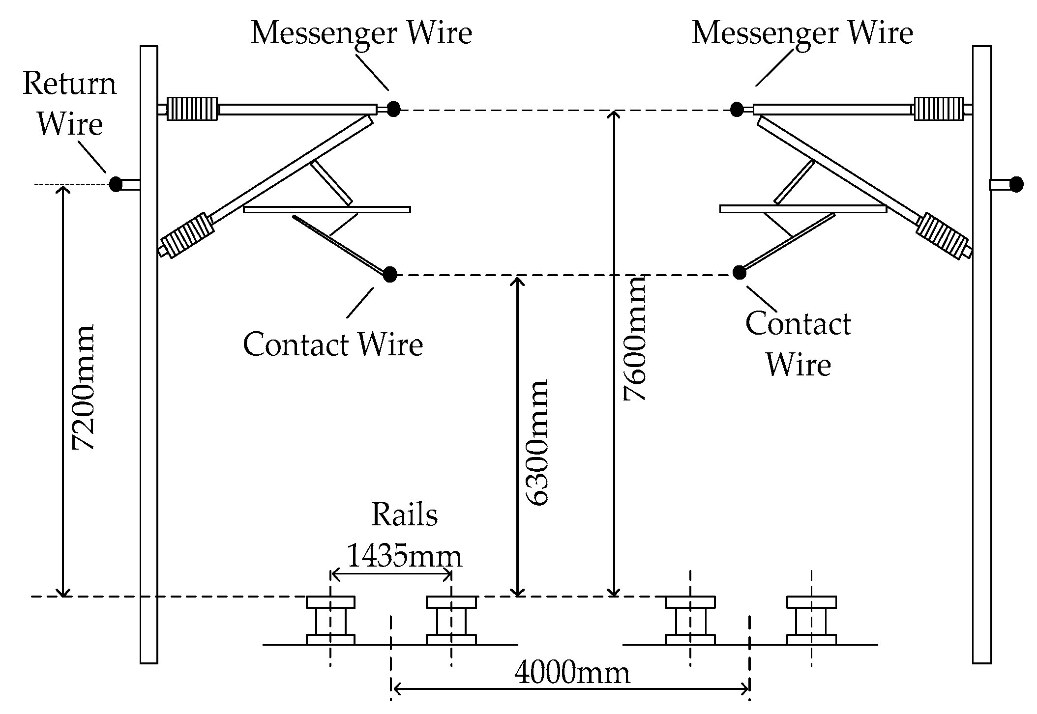
Energies 11 02255 g009
Figure 10. Relative positions between the electrified railways and buried pipelines.
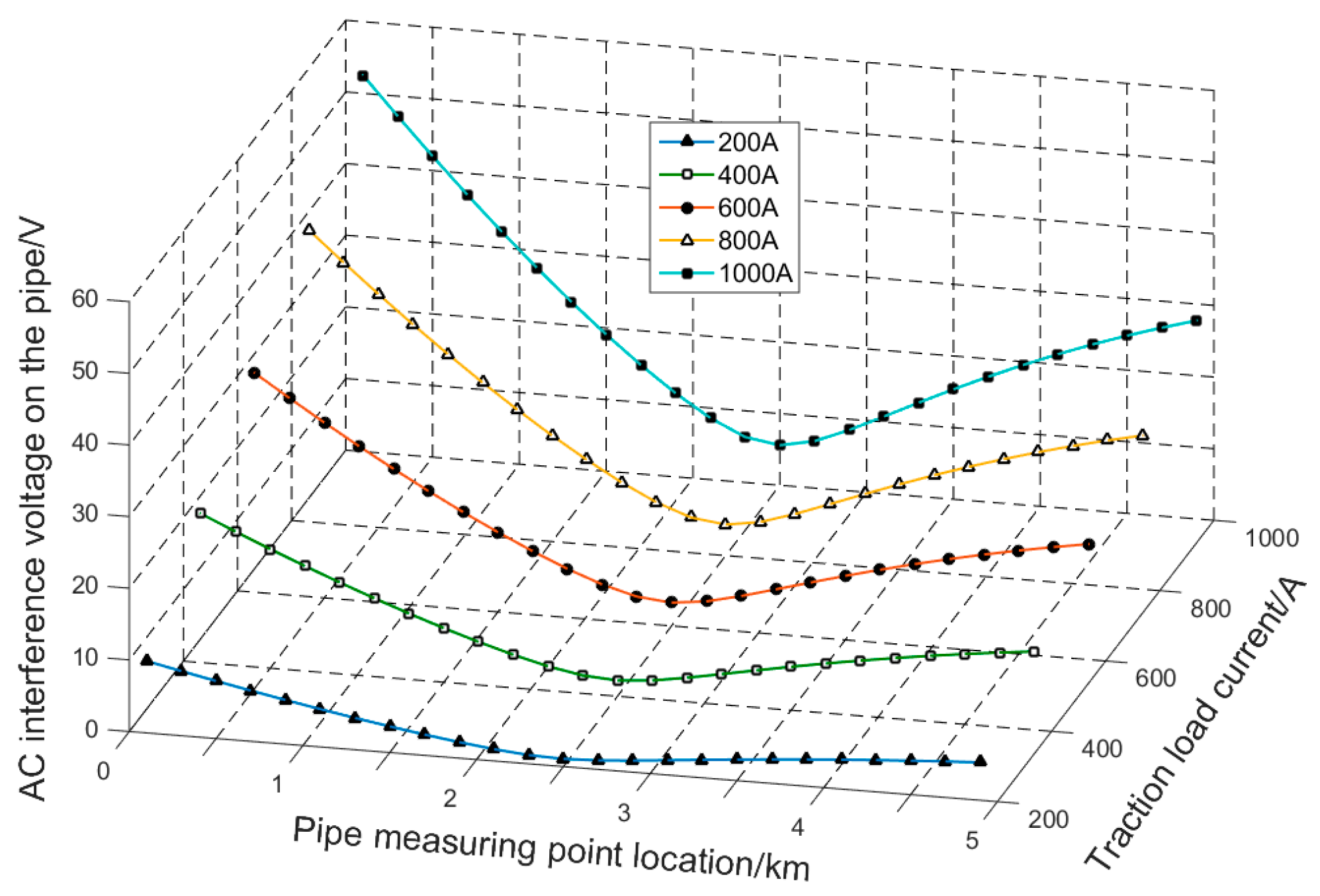
Energies 11 02255 g010
Figure 11. Influence of traction load current on AC interference voltage distribution on the pipeline.
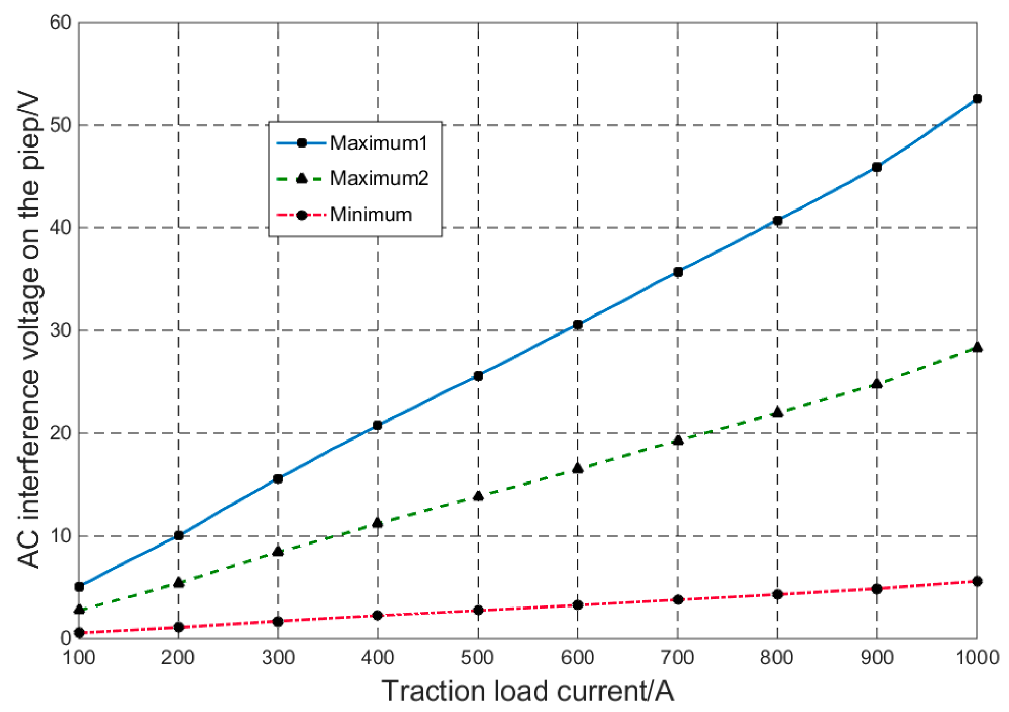
Energies 11 02255 g011
Figure 12. The distribution of AC interference voltages on the pipeline with different traction load current.
Energies 11 02255 g012
Figure 13. Influence of traction load location on AC interference voltage distribution on the pipeline.
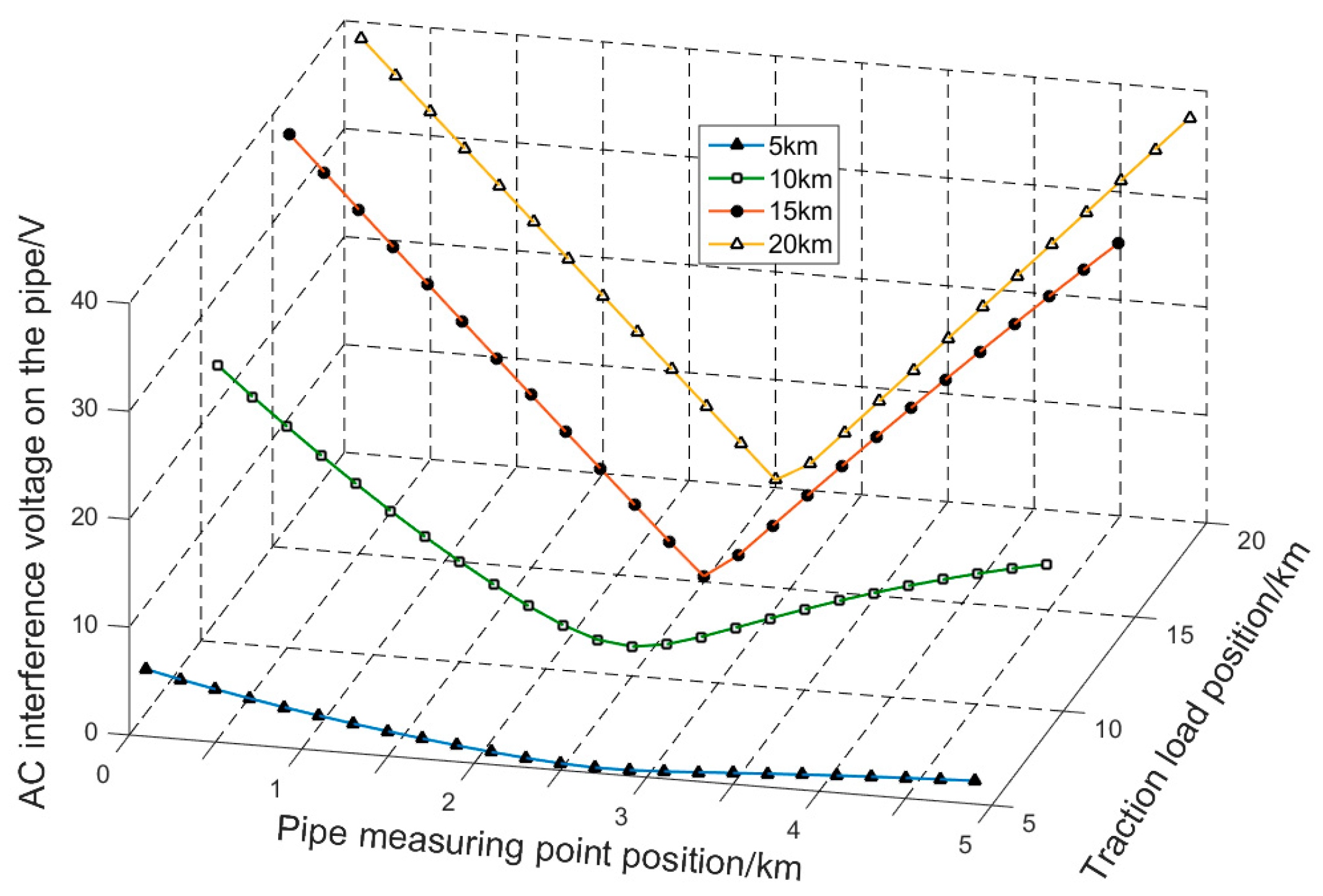
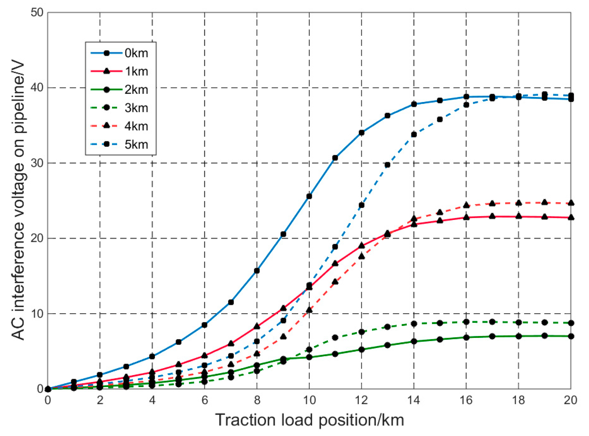
Energies 11 02255 g013
Figure 14. The distribution of AC interference voltages on the pipeline with different traction load position.
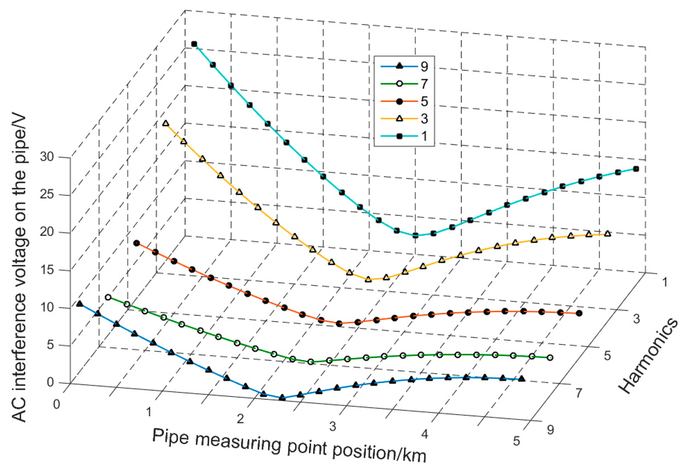
Energies 11 02255 g014
Figure 15. Influence of harmonics on the AC interference voltage distribution on the pipeline.
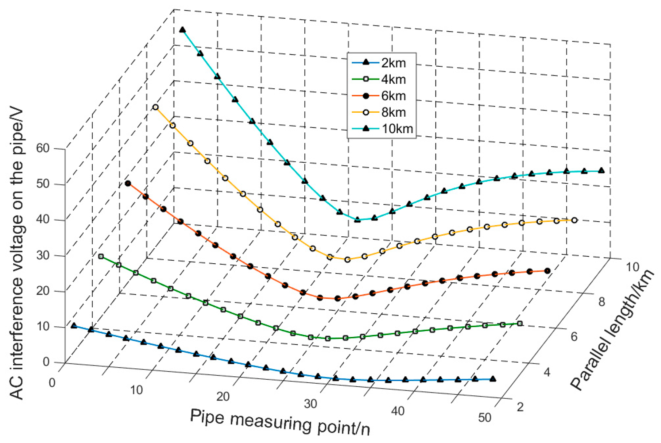
Energies 11 02255 g015
Figure 16. Influence of parallel length on AC interference voltage distribution on the pipeline.
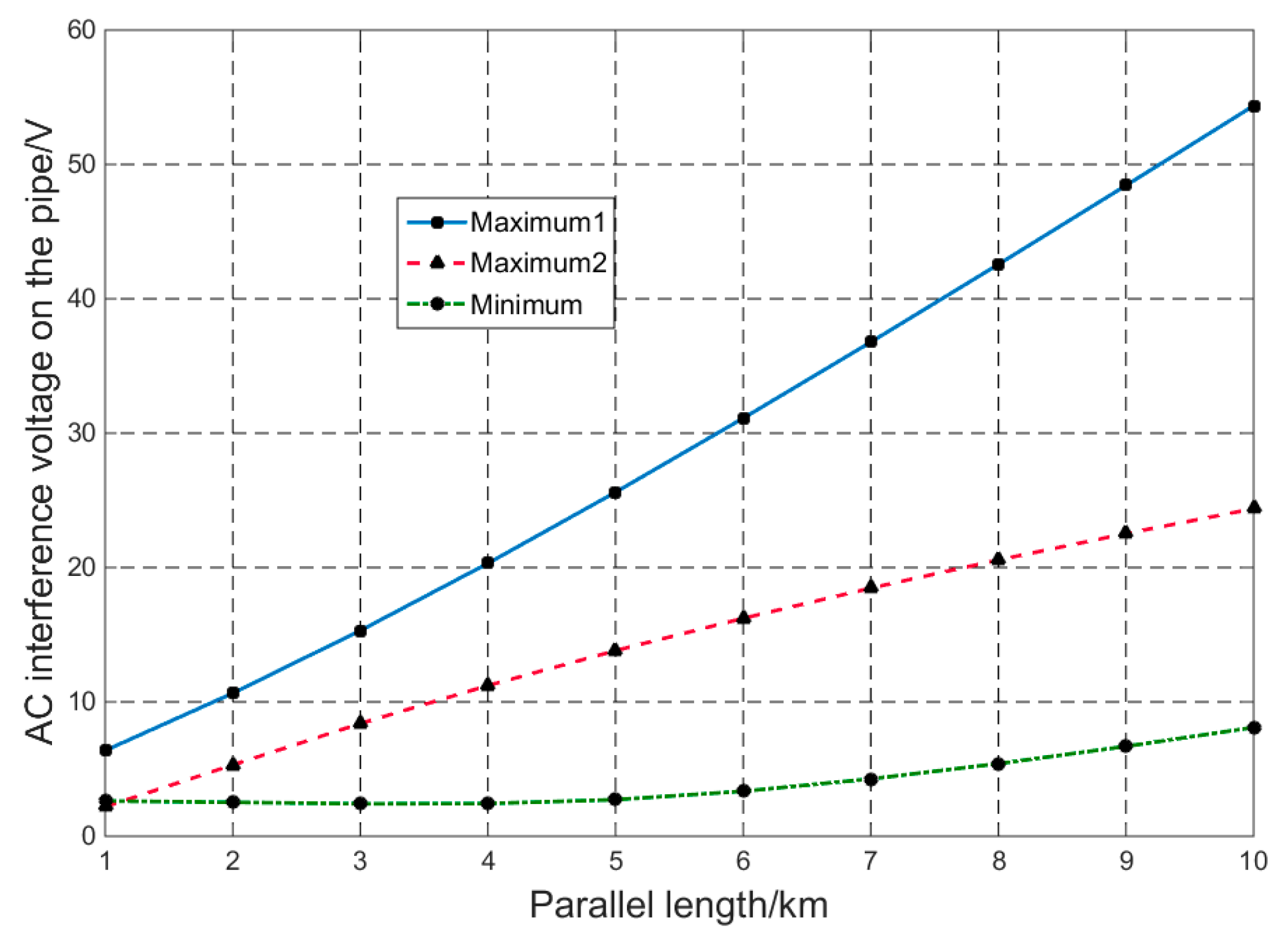
Energies 11 02255 g016
Figure 17. The distribution of AC interference voltages of the pipeline with different parallel lengths.
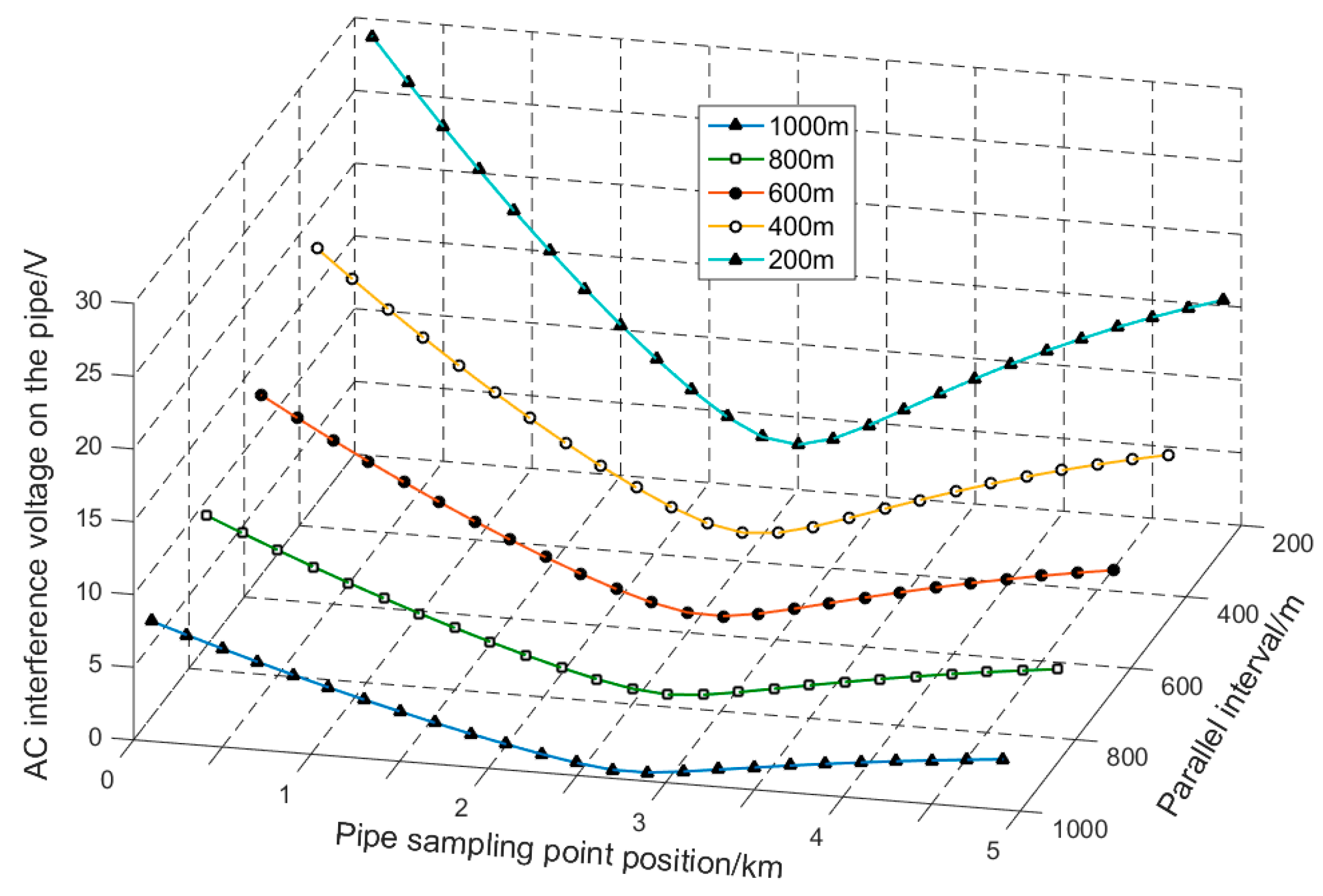
Energies 11 02255 g017
Figure 18. Influence of parallel interval on AC interference voltage distribution on the pipeline.
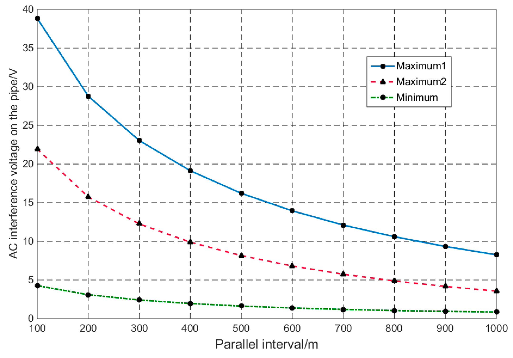
Energies 11 02255 g018
Figure 19. The distribution of AC interference voltages of the pipeline with different parallel intervals.
Energies 11 02255 g019
Figure 20. Influence of pipe coatings on AC interference voltage distribution on the pipeline.
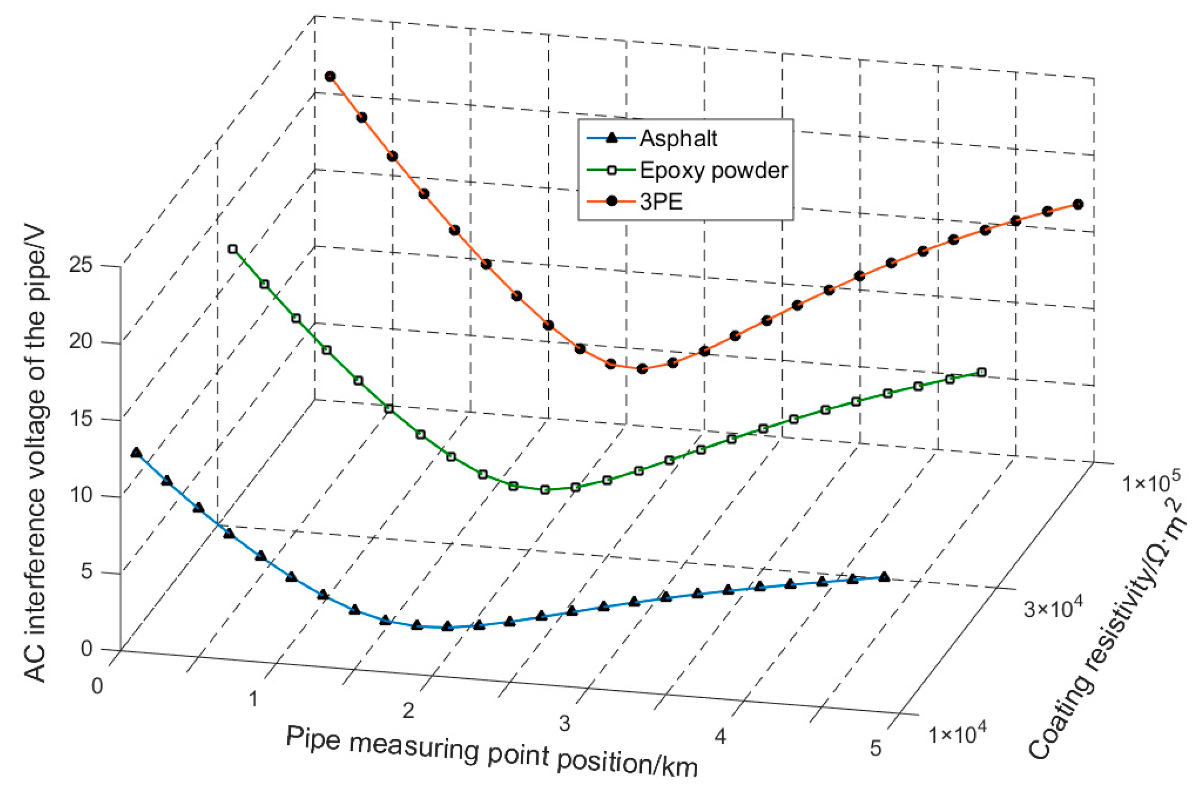
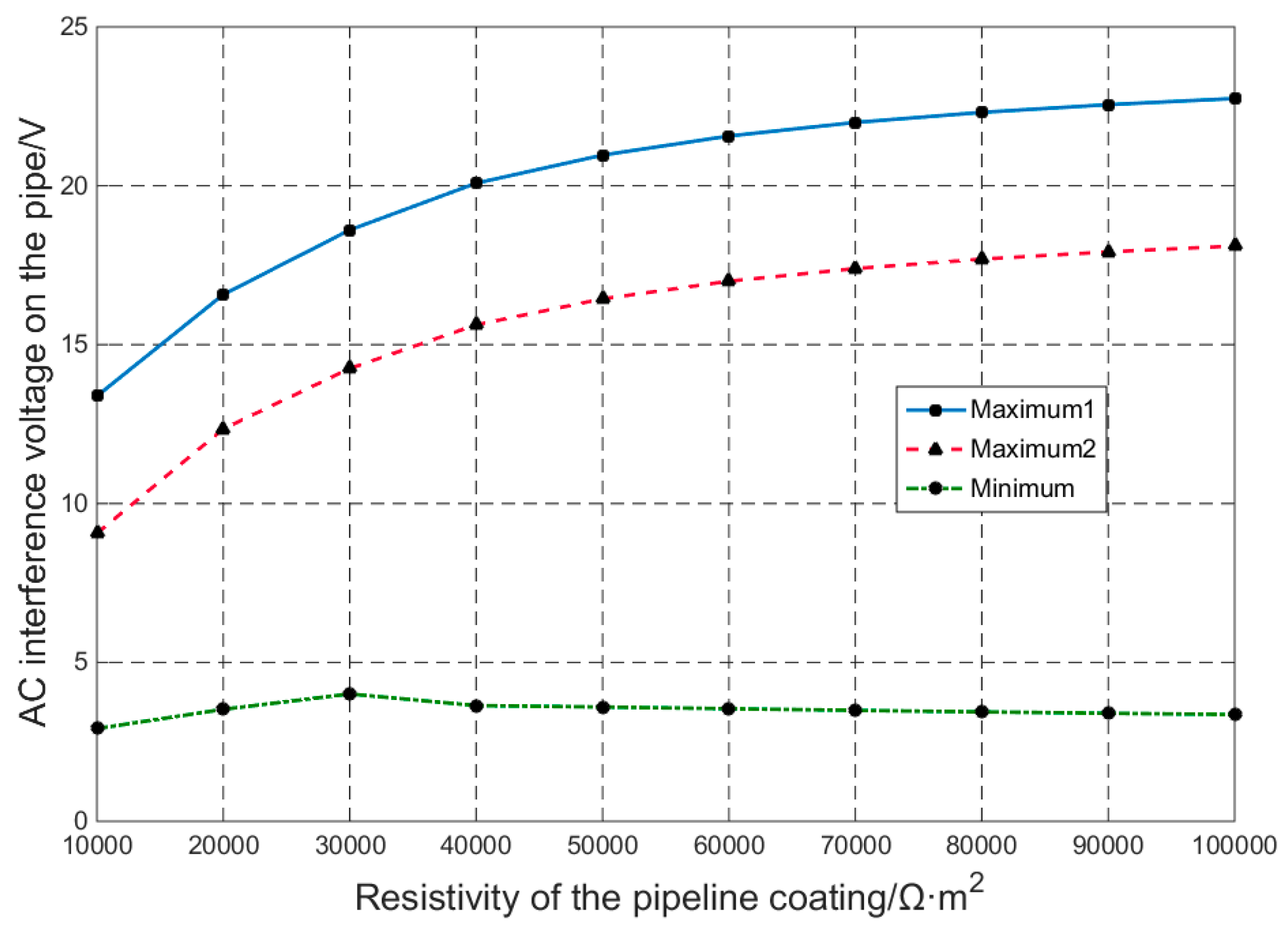
Energies 11 02255 g020
Figure 21. The distribution of AC interference voltages of the pipeline with different coating resistances.
Energies 11 02255 g021
Figure 22. Influence of soil resistance on AC interference voltage distribution.
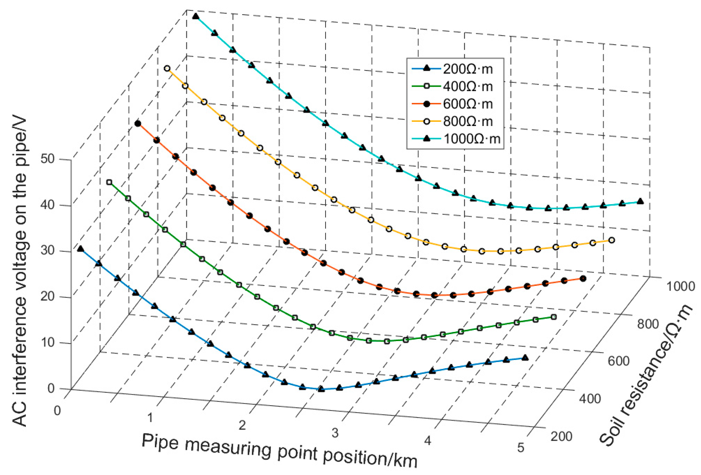
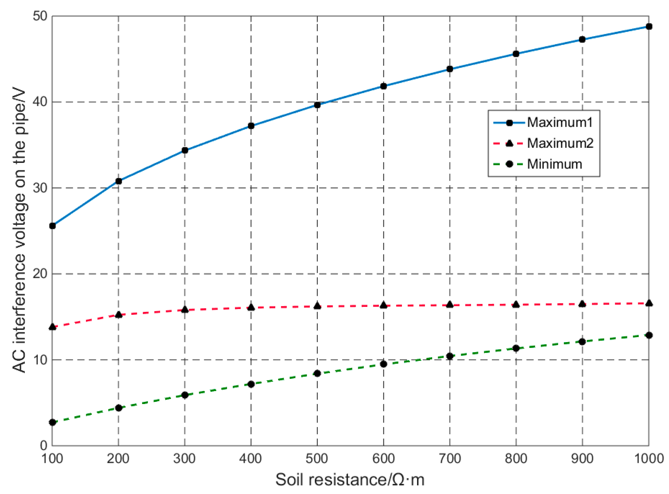
Energies 11 02255 g022
Figure 23. The distribution of AC interference voltages of the pipeline with different soil resistances.
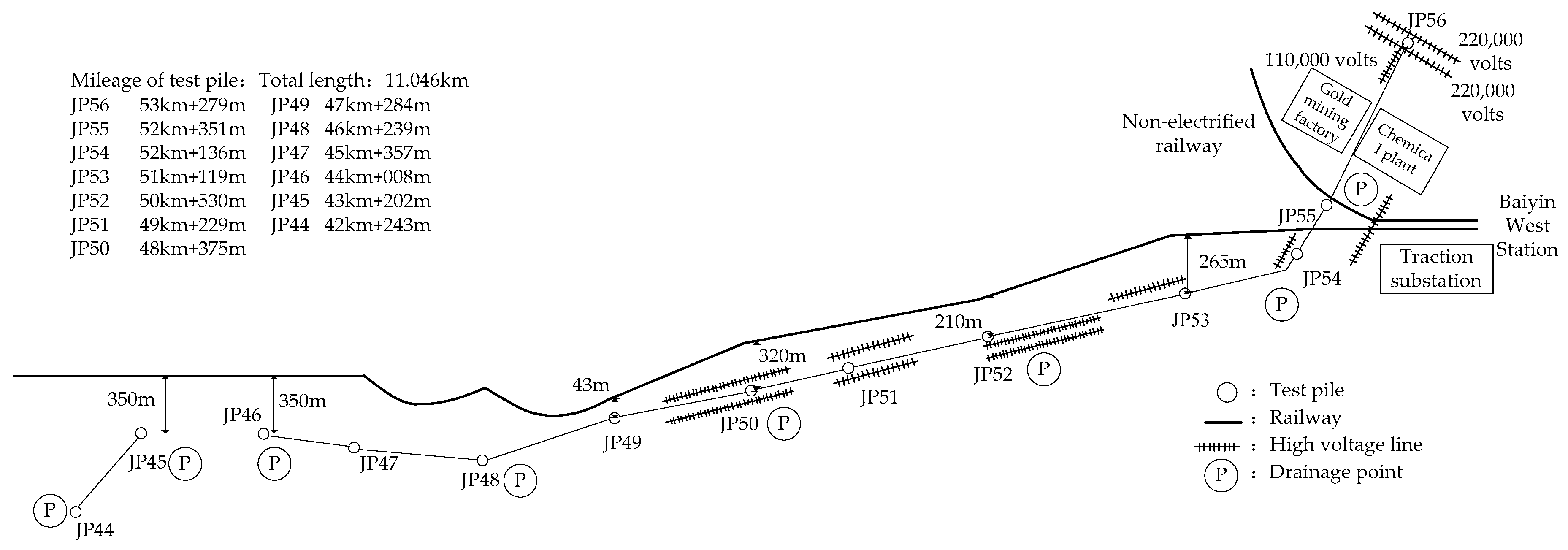
Energies 11 02255 g023
Figure 24. Schematic diagram of the Baolan railway and the Baiyin branch pipeline.
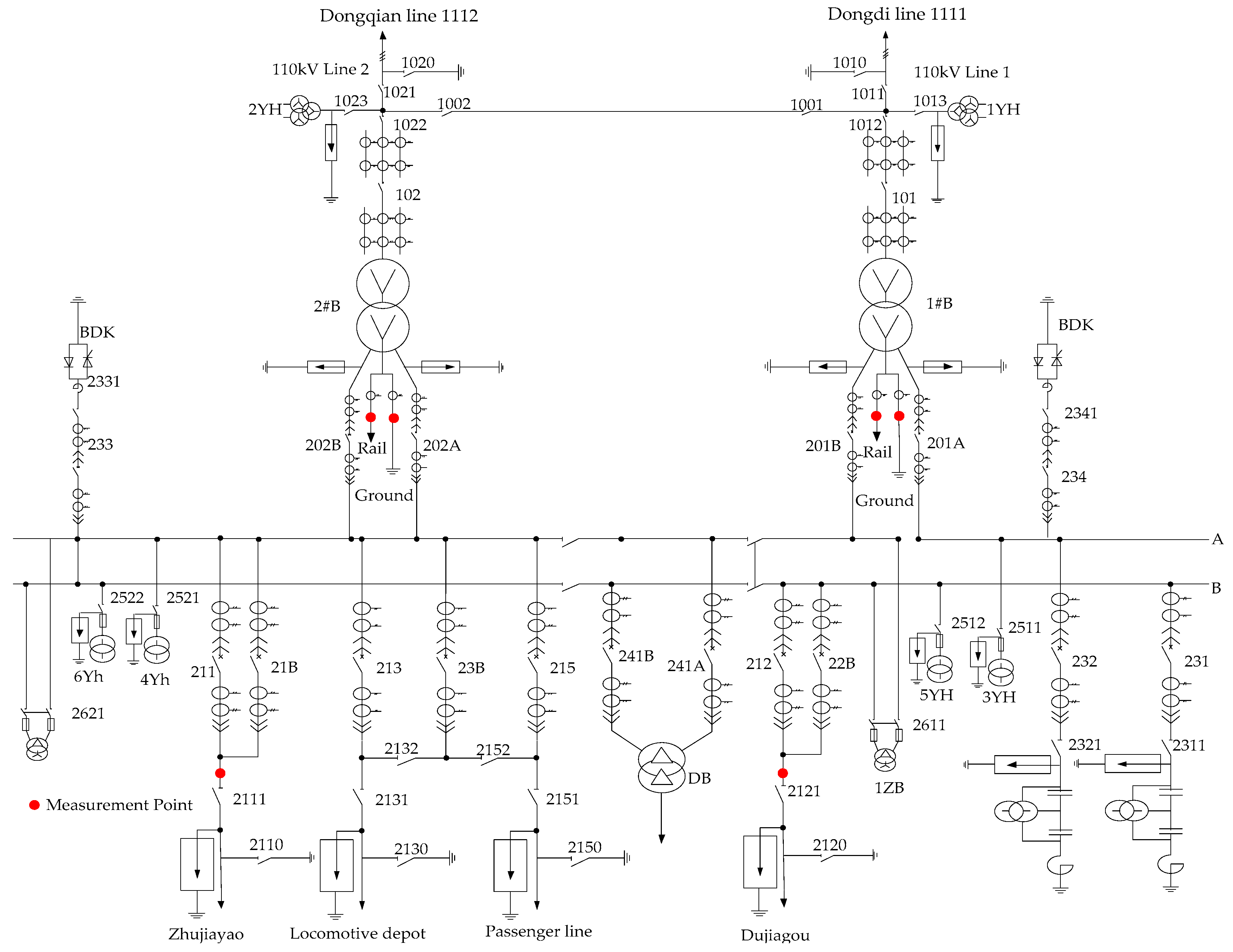
Energies 11 02255 g024
Figure 25. Electrical diagram of the Baiyin West traction substation.
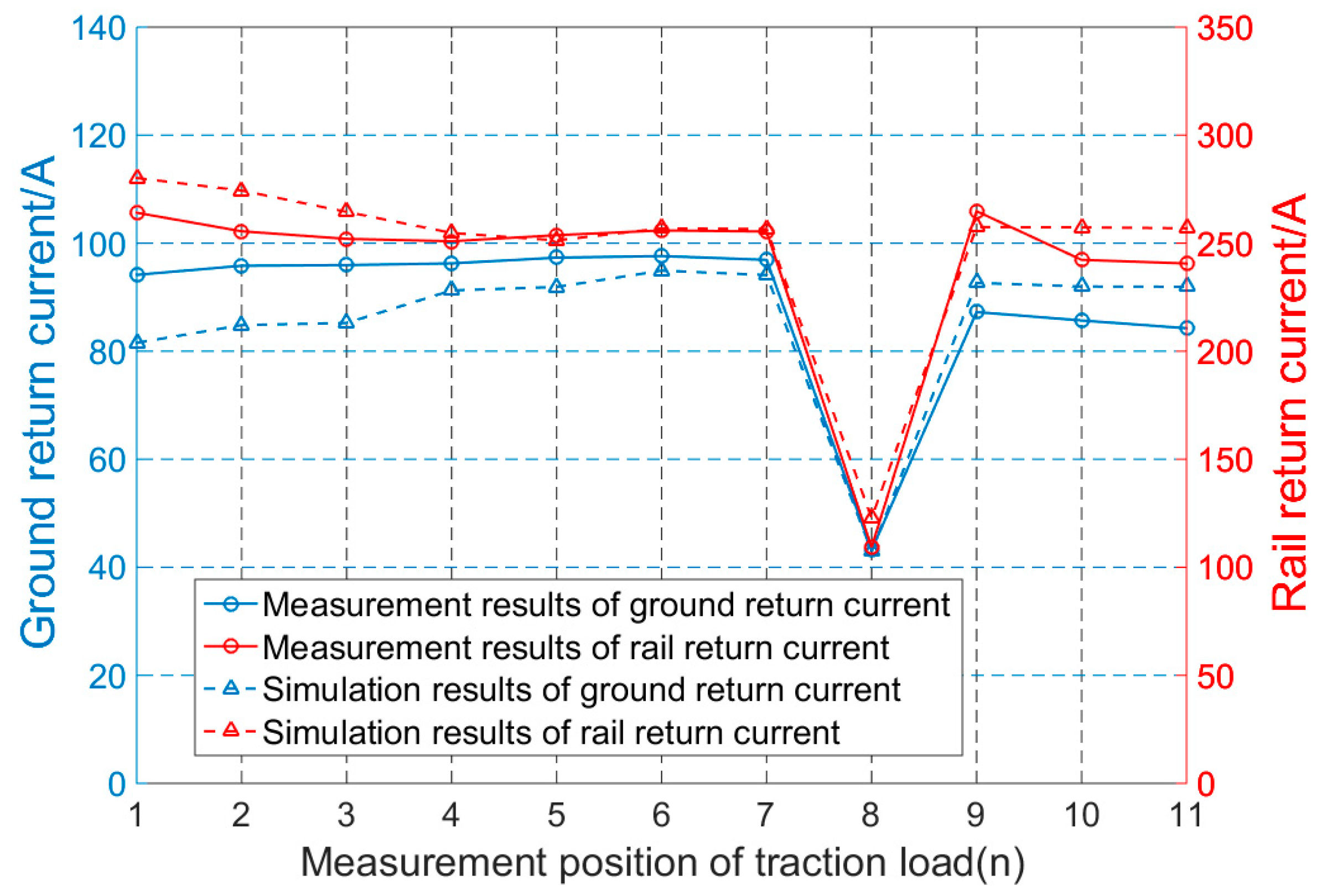
Energies 11 02255 g025
Figure 26. The results of the traction return current (traction load current is 350 A).
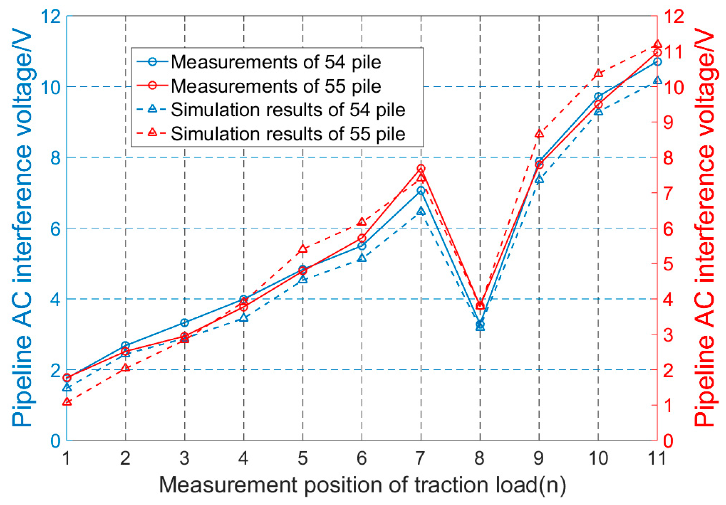
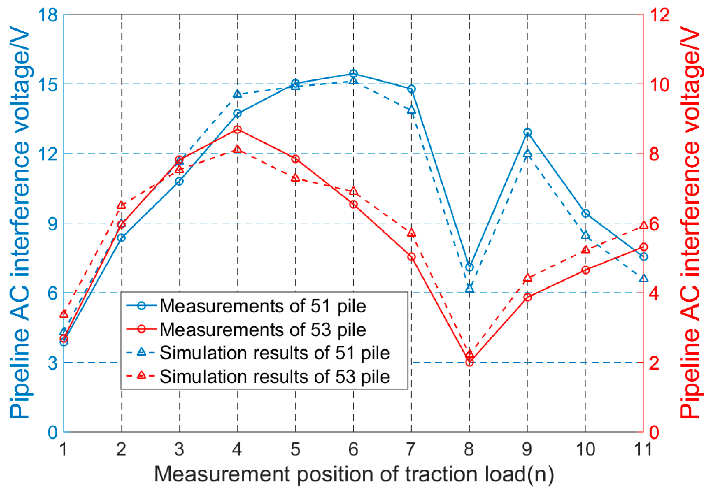
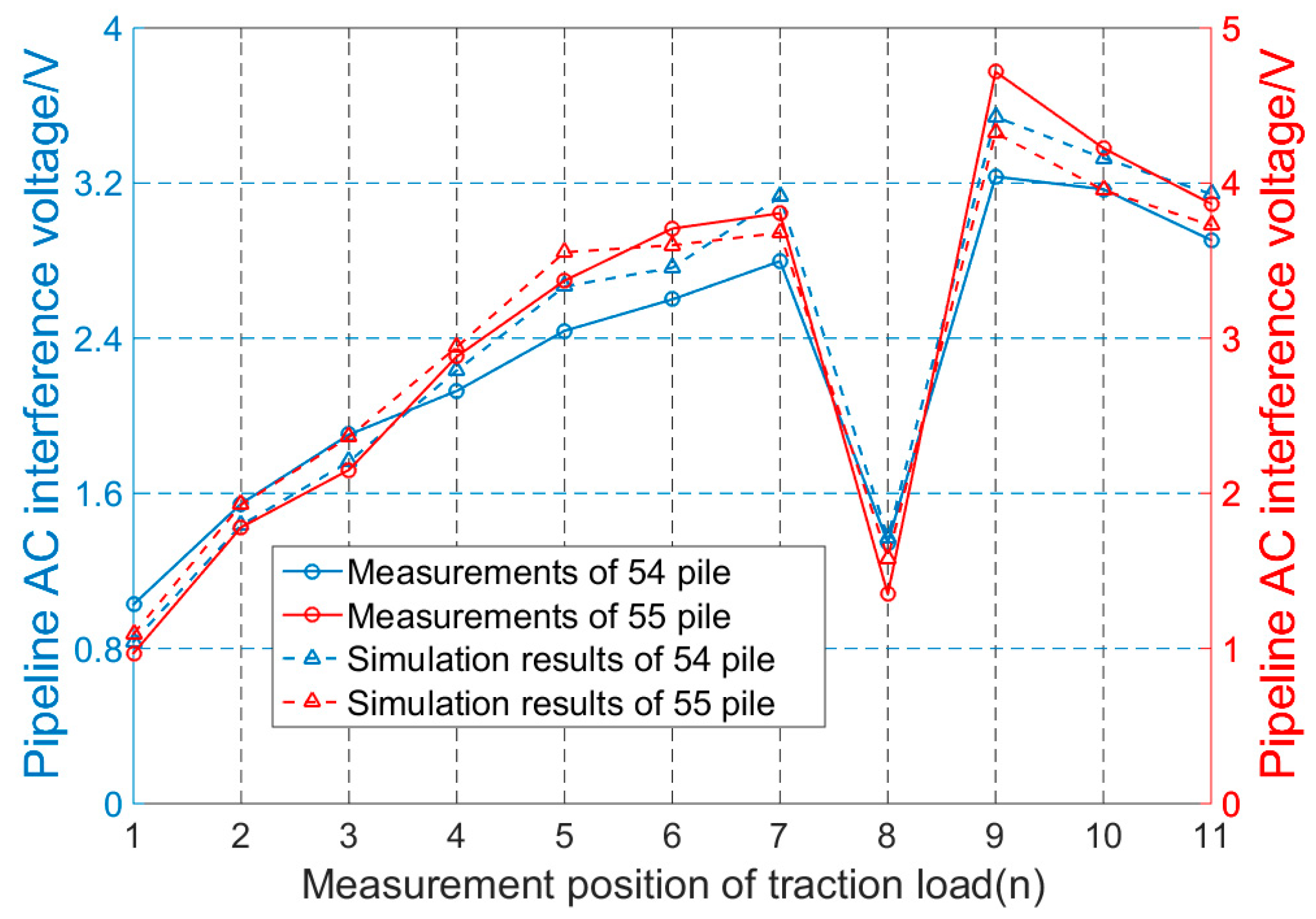
Energies 11 02255 g026
Figure 27. Comparison of measurement and simulation of the undraining condition in the cross section.
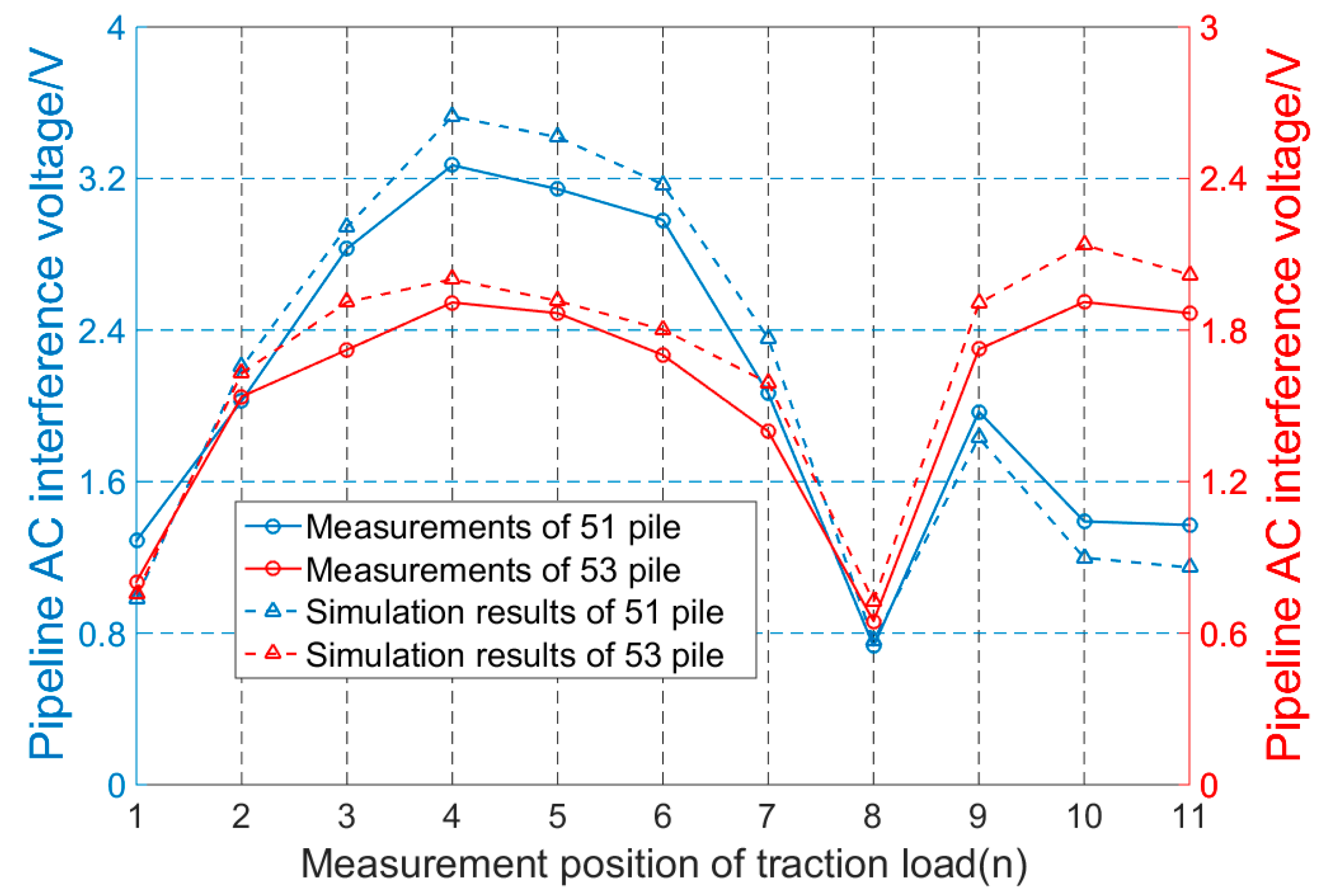
Energies 11 02255 g027
Figure 28. Comparison of measurement and simulation of the undraining condition in the parallel section.
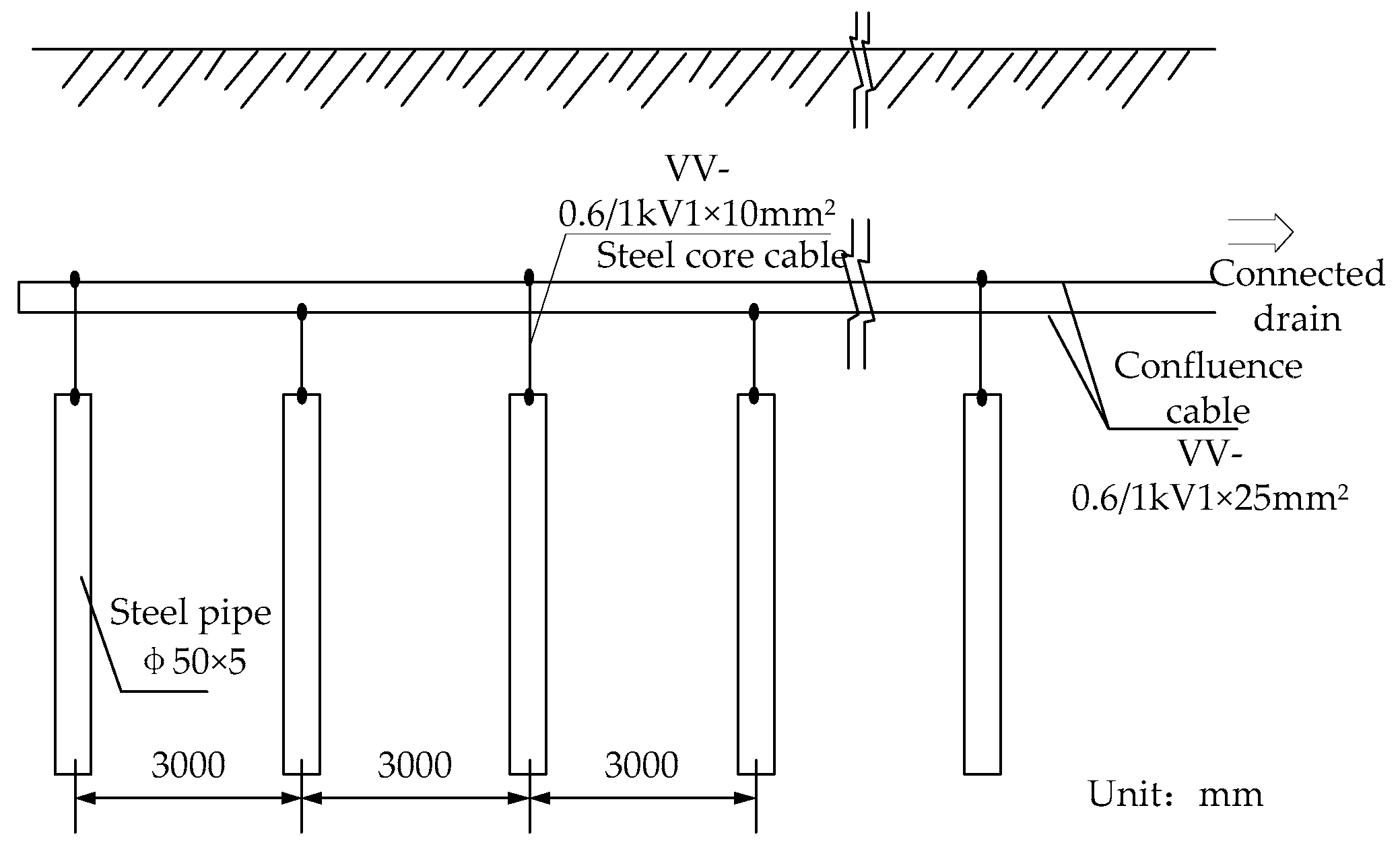
Energies 11 02255 g028
Figure 29. Schematic diagram of the ground pole structure of the drainage device.
Energies 11 02255 g029
Figure 30. Comparison of measurement and simulation of the draining condition in the cross section.
Energies 11 02255 g030
Figure 31. Comparison of measurement and simulation of the draining condition in the parallel section.
Energies 11 02255 g031
Table 1. Parameters of the traction transformer.
ParameterCharacteristics
Capacity (MVA)40
Ratio220/27.5
Short circuit impedance (%)8.4
Table 2. Parameters of the grounding grid.
CategoryParameterCharacteristics
Horizontal grounding gridArea150 × 150 m
Conductor materialGalvanized flat steel
Conductor spacing20 m
Vertical grounding conductorLength2.5 m
Conductor materialGalvanized angle steel
Conductor spacing7.5 or 15 m
Grounding gridEarthing impedance0.3 Ω
Table 3. Parameters of the rail (P60).
Specification (kg/m)Weight (kg/m)Section (cm2)Calculate Radius (mm)Effective Internal Resistance (Ω/km)Equivalent Radius (mm)
6060.3577.08109.10.13512.79
Table 4. Buried pipeline parameters.
ParameterCharacteristics
Pipe diameter (mm)508
Wall thickness (mm)12
Coating material3 PE
Coating thickness (mm)3.3
Coating resistivity ( Ω · m )100,000
Pipeline relative resistivity (relative to copper)10
Relative permeability of pipeline300
Buried depth (m)2
Table 5. Short circuit impedance of traction power supply system.
The Distance between the Short Circuit Point and the Traction Substation (km)CDEGSCarson TheoryError (%)
10.6350.6074.61
106.2316.0293.35
159.279.0412.53
2012.2712.051.83
Table 6. Simulation and calculation results of inductive coupling and resistive coupling voltages on buried pipelines.
The Horizontal Distance of the Buried Pipeline from the Center Point of the Line (m)Inductive Coupling Calculation (Potential Maximum Point)Resistive Coupling Calculation (Positive to Discharge Point)
Simulation Value (V)Calculated Value (V)Error (%)Simulation Value (V)Calculated Value (V)Error (%)
3054.76650.8667.6674.0963.8735.758
5048.59945.2847.3213.6983.5145.231
10038.87336.4166.7463.173.0145.168
15032.98631.2215.6542.8482.7244.537
30023.05822.1564.0692.272.2013.144
50016.22815.6363.7881.851.8251.375
Table 7. Harmonic current data of AC-DC electric locomotive.
f/HznAmplitude of Harmonic Current (A)Harmonic Content (%)
501500100
1503183.136.62
250557.0511.41
350732.206.44
450943.408.68
Table 8. Parameters of AC Interference Voltage Test Point.
Test PilePosition Relation with RailwayDistance from Railway (m)
45Parallel322
46Parallel334
47Parallel676
48Parallel575
49Parallel42
50Parallel300
51Parallel400
52Parallel202
53Parallel223
54Cross68.5
55Cross91.2
Table 9. Parameters of the traction transformer.
ParameterCharacteristics
Transformer windingsVv
Capacity (MVA)20
Ratio110/27.5
Short circuit impedance (%)10.54
No-load current (%)0.15
No-load loss (kW)26.855
Sheath losses (kW)176.795
Table 10. The grounding resistance values of the Baiyin branch discharge devices.
The number of installation locations444546484951535456
Grounding resistance value (Ω)1.51.1121.221.821.9

