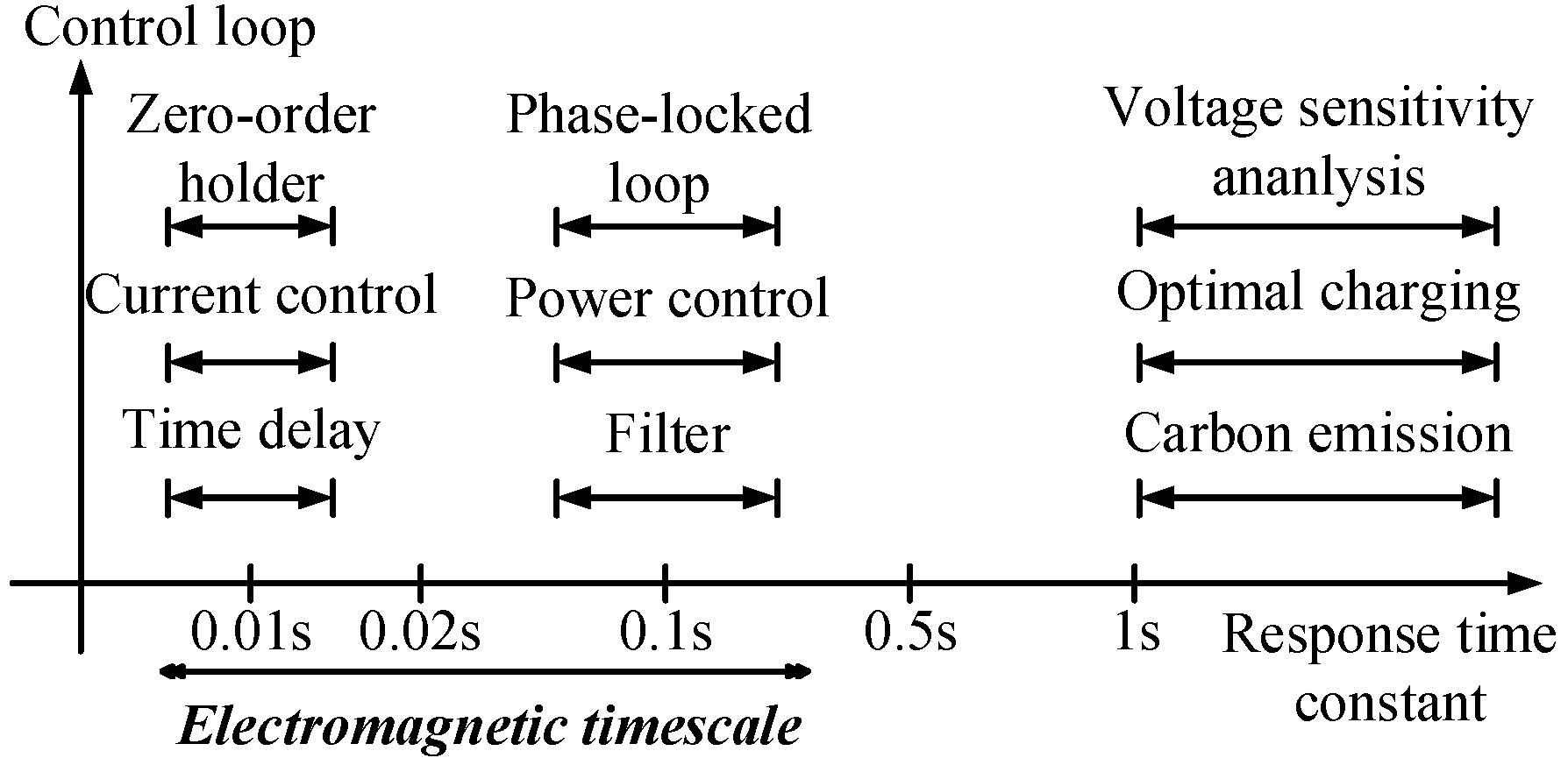
Figure 1.
Extending the multi-timescale classification of a power electronic converter.
Figure 1.
Extending the multi-timescale classification of a power electronic converter.
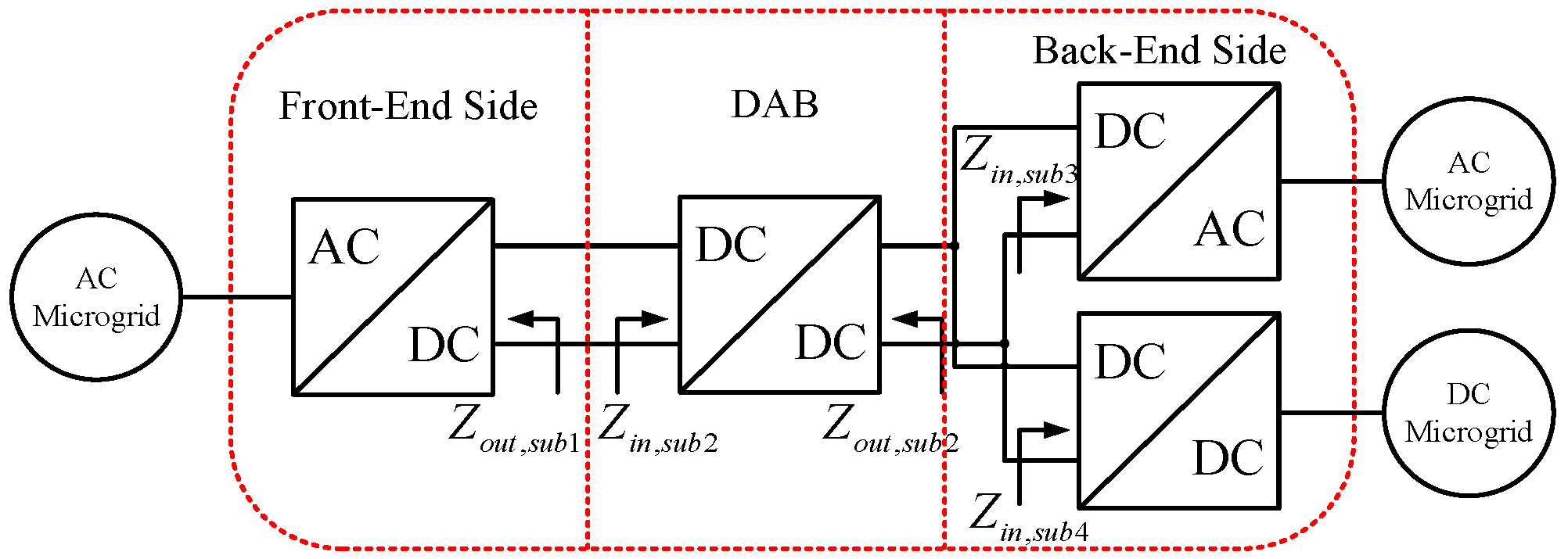
Figure 2.
The multi-port single-phase solid-state transformer (MS3T) structure model with three stages.
Figure 2.
The multi-port single-phase solid-state transformer (MS3T) structure model with three stages.
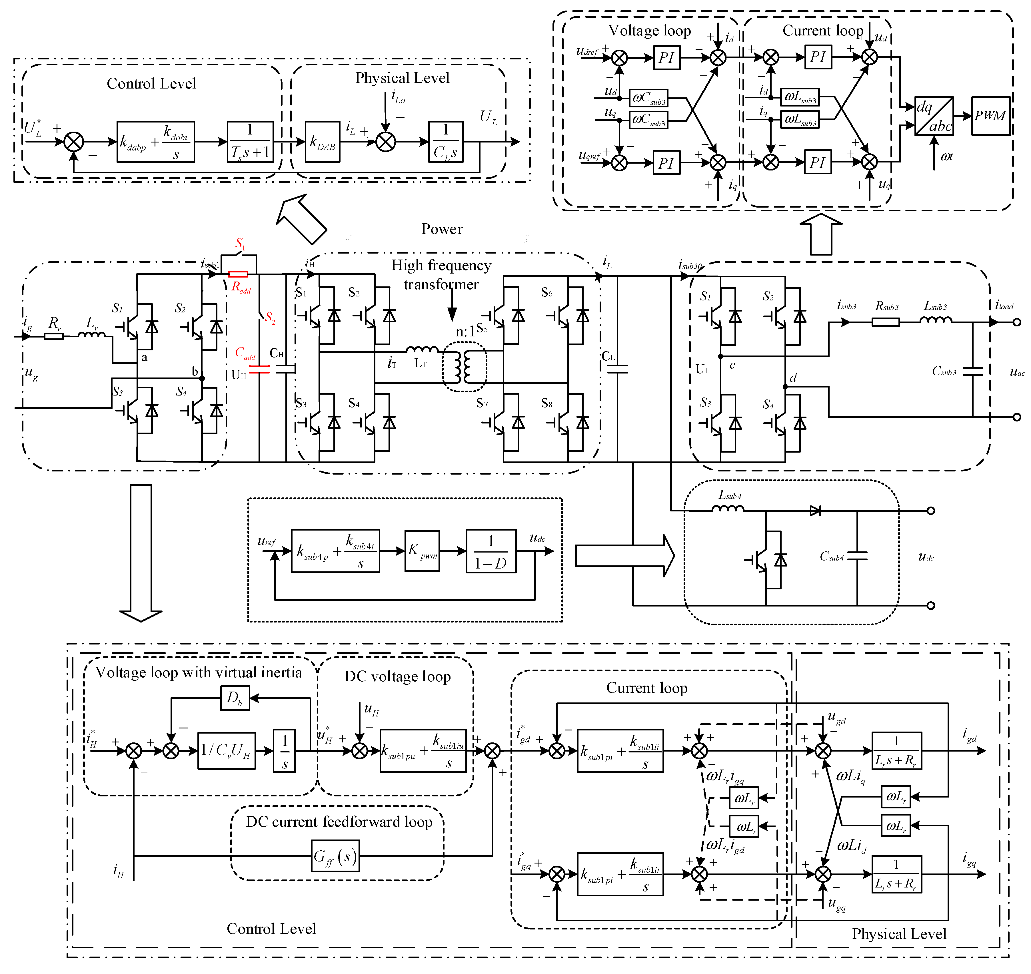
Figure 3.
The overall control strategy and topological structure of the MS3T.
Figure 3.
The overall control strategy and topological structure of the MS3T.
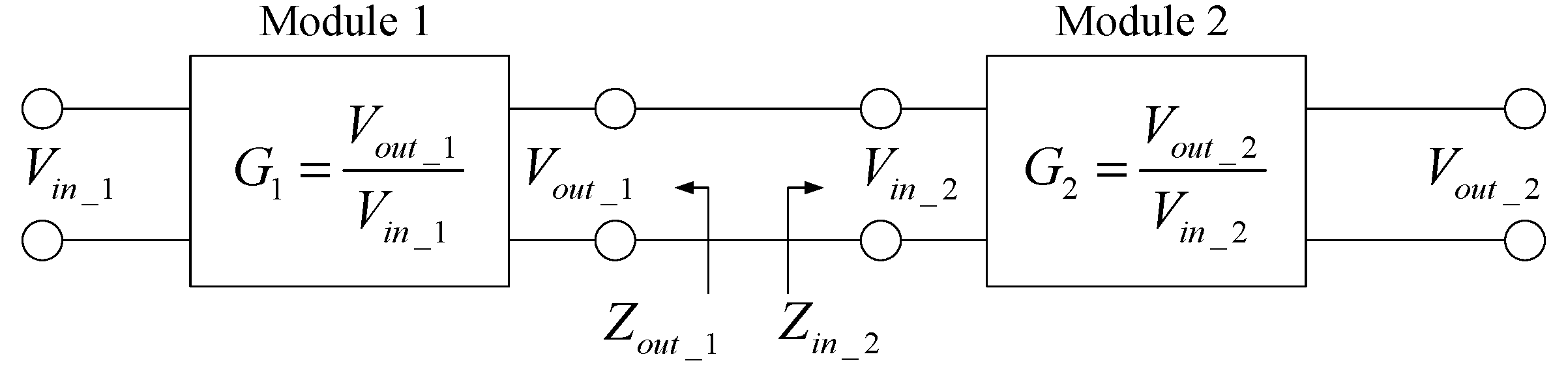
Figure 4.
Interconnection of two stable independent systems.
Figure 4.
Interconnection of two stable independent systems.
Figure 5.
Setup for the terminal characterization of the MS3T.
Figure 5.
Setup for the terminal characterization of the MS3T.
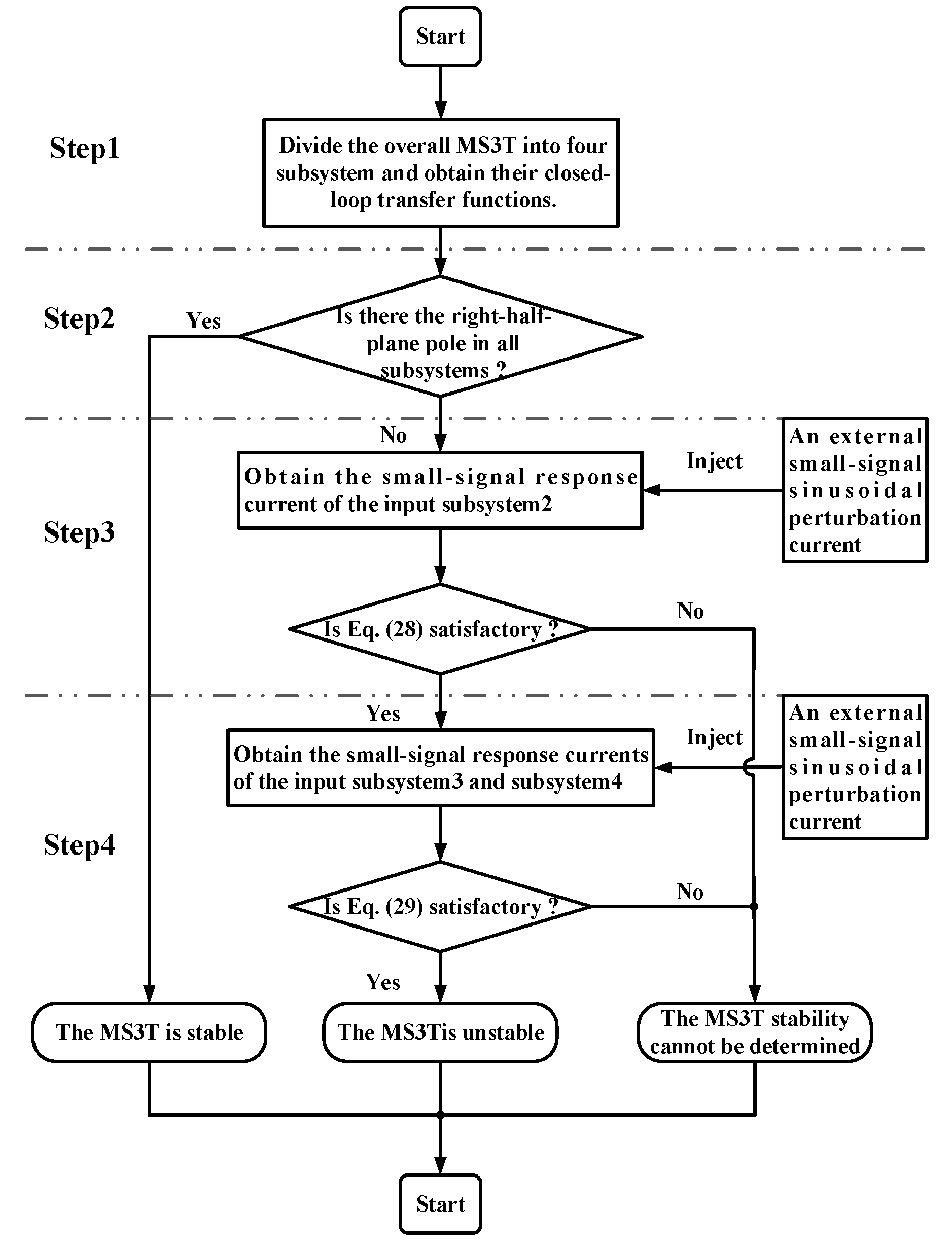
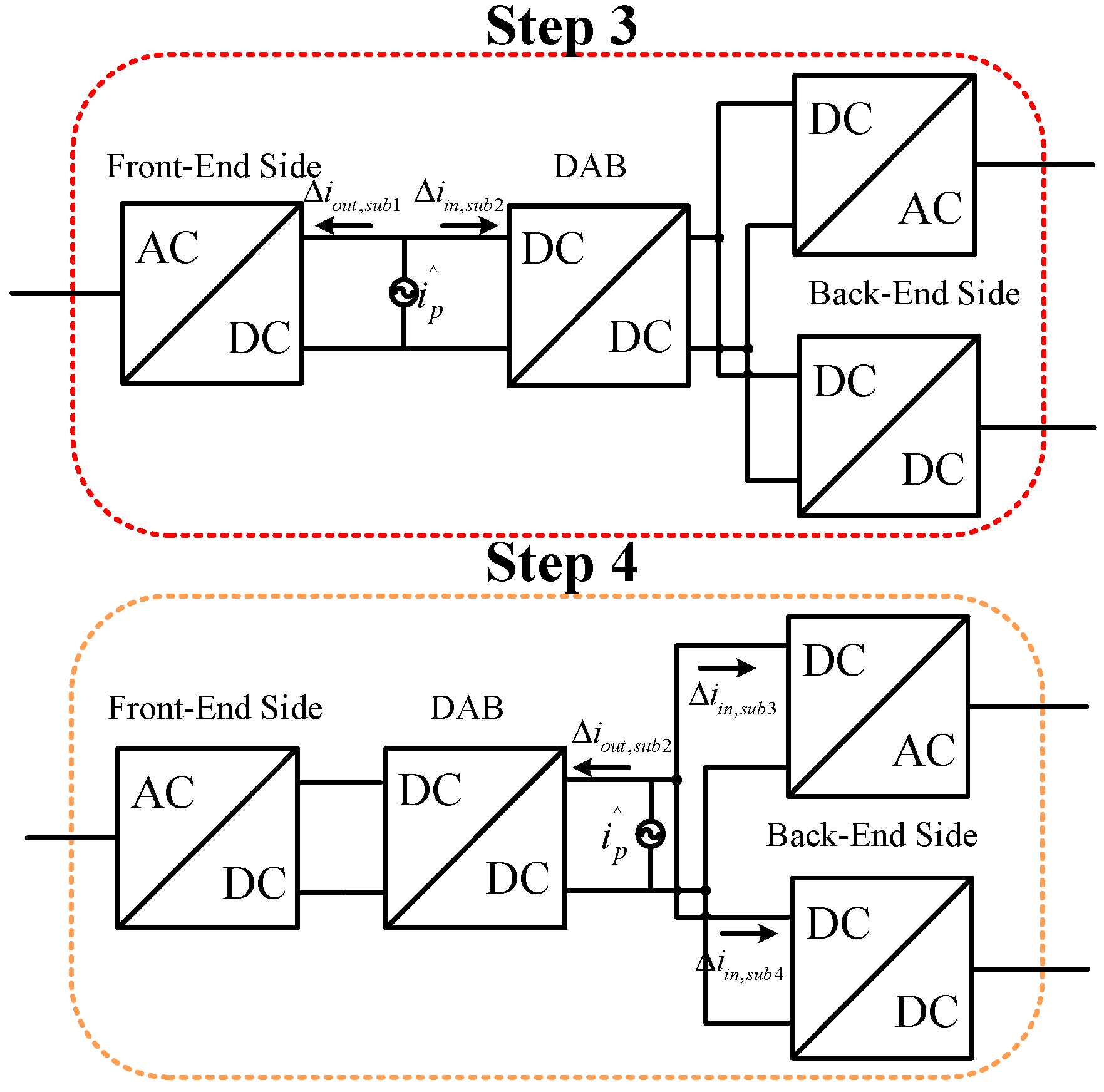
Figure 6.
The flow chart of the proposed stability assessment method.
Figure 6.
The flow chart of the proposed stability assessment method.
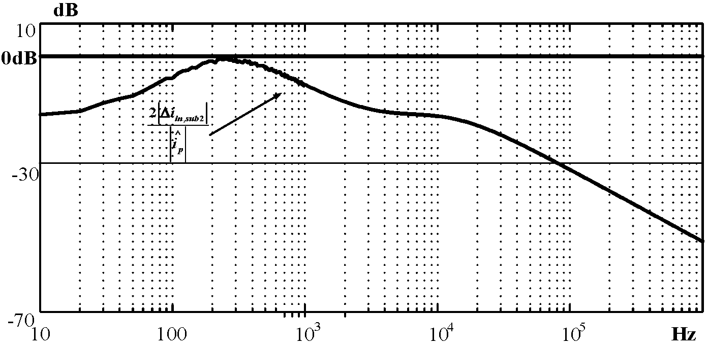
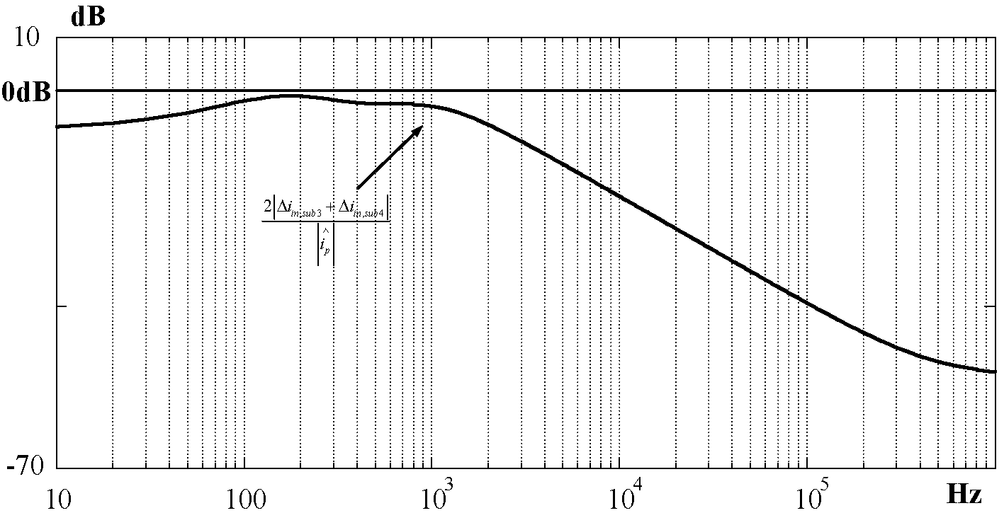
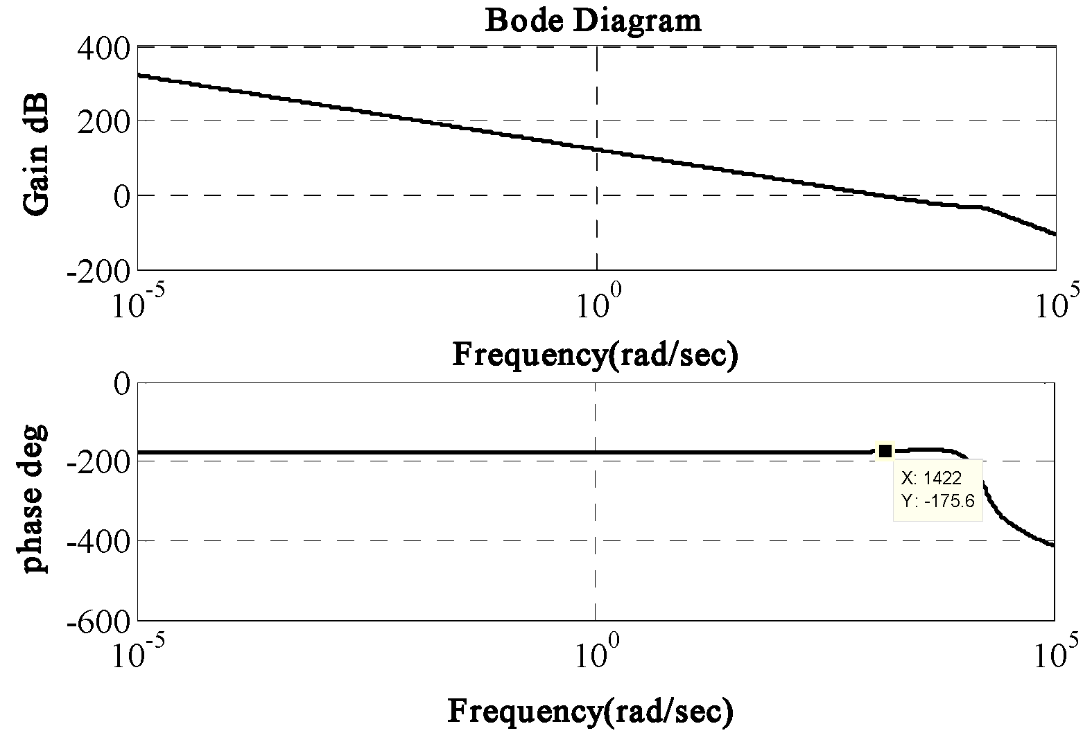
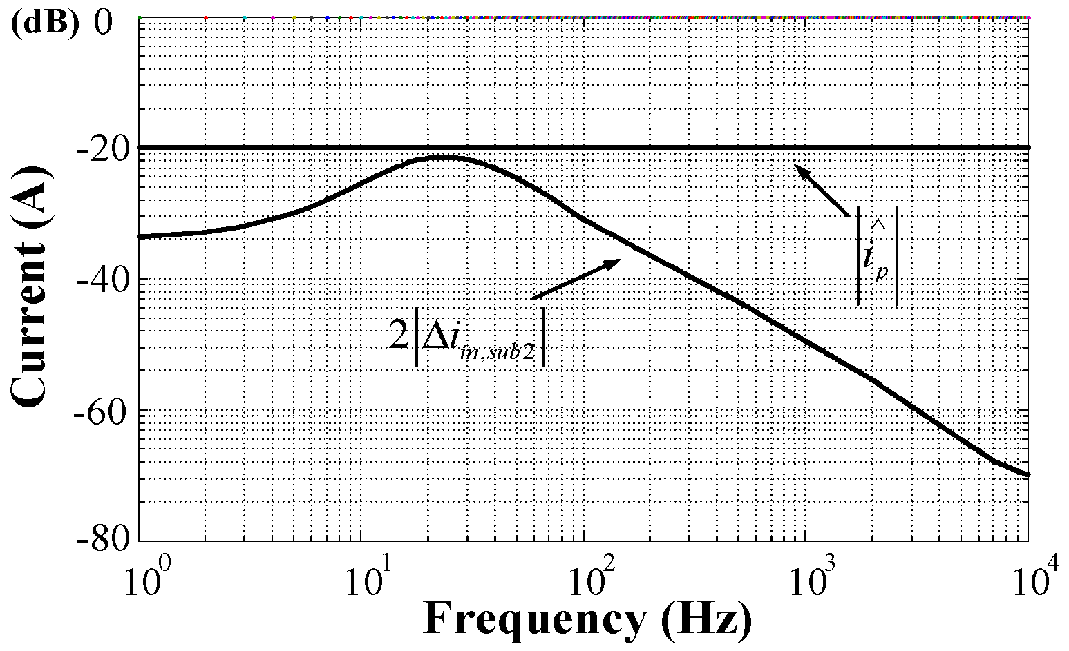
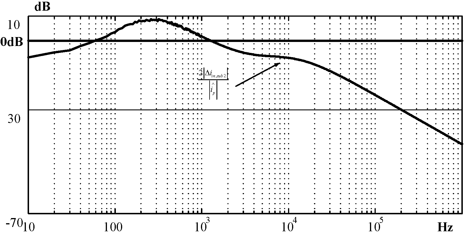
Figure 7.
The Bode diagram of the DC-AC back-end side converter.
Figure 7.
The Bode diagram of the DC-AC back-end side converter.
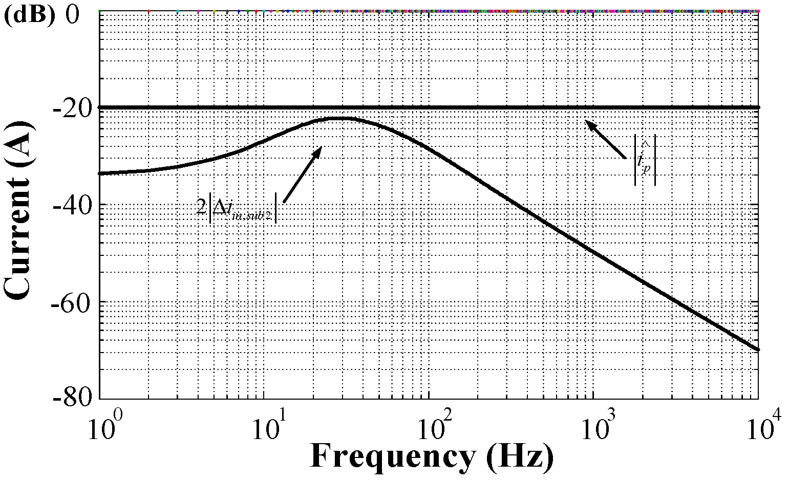
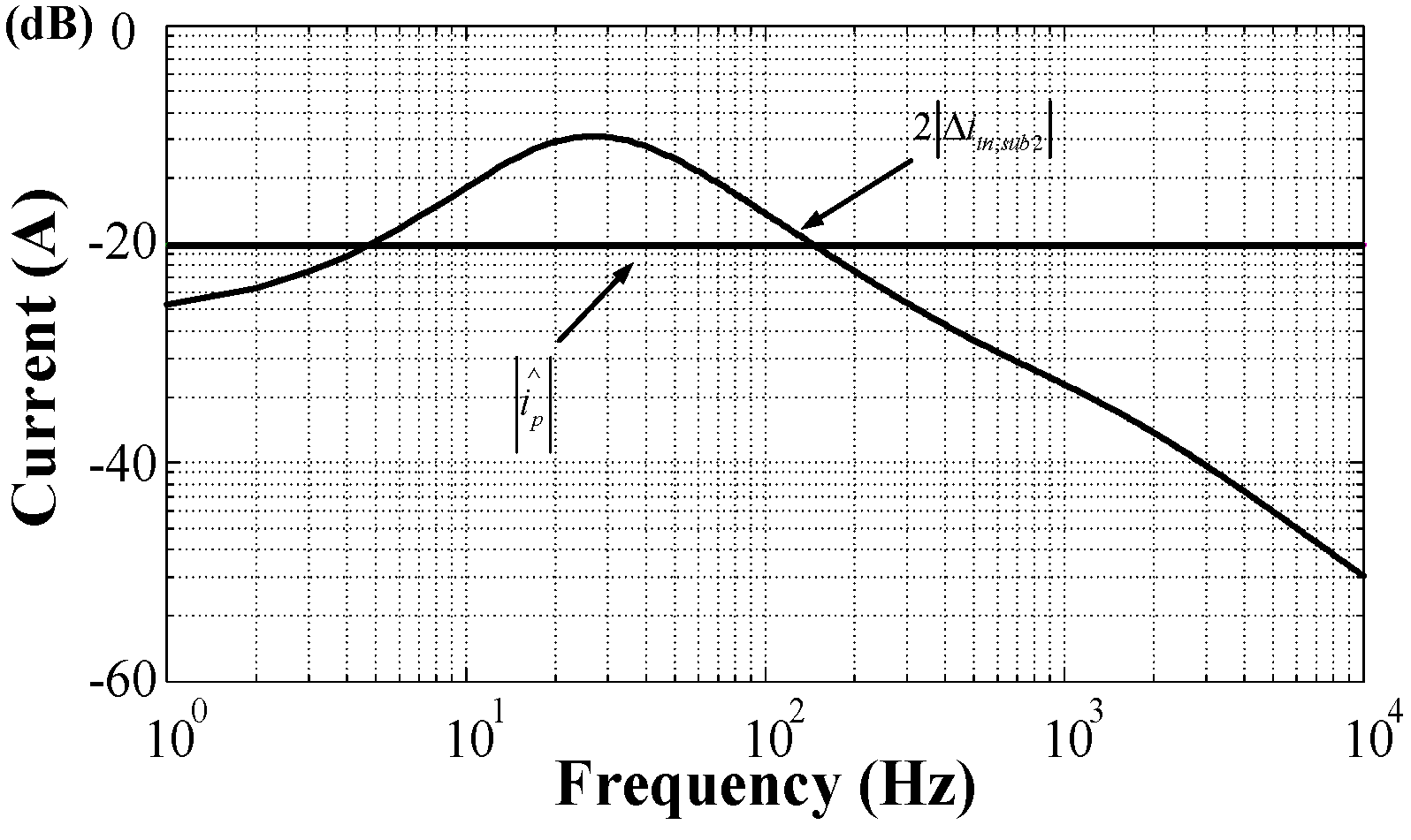
Figure 8.
Relationship between measured currents of and in a stable case.
Figure 8.
Relationship between measured currents of and in a stable case.
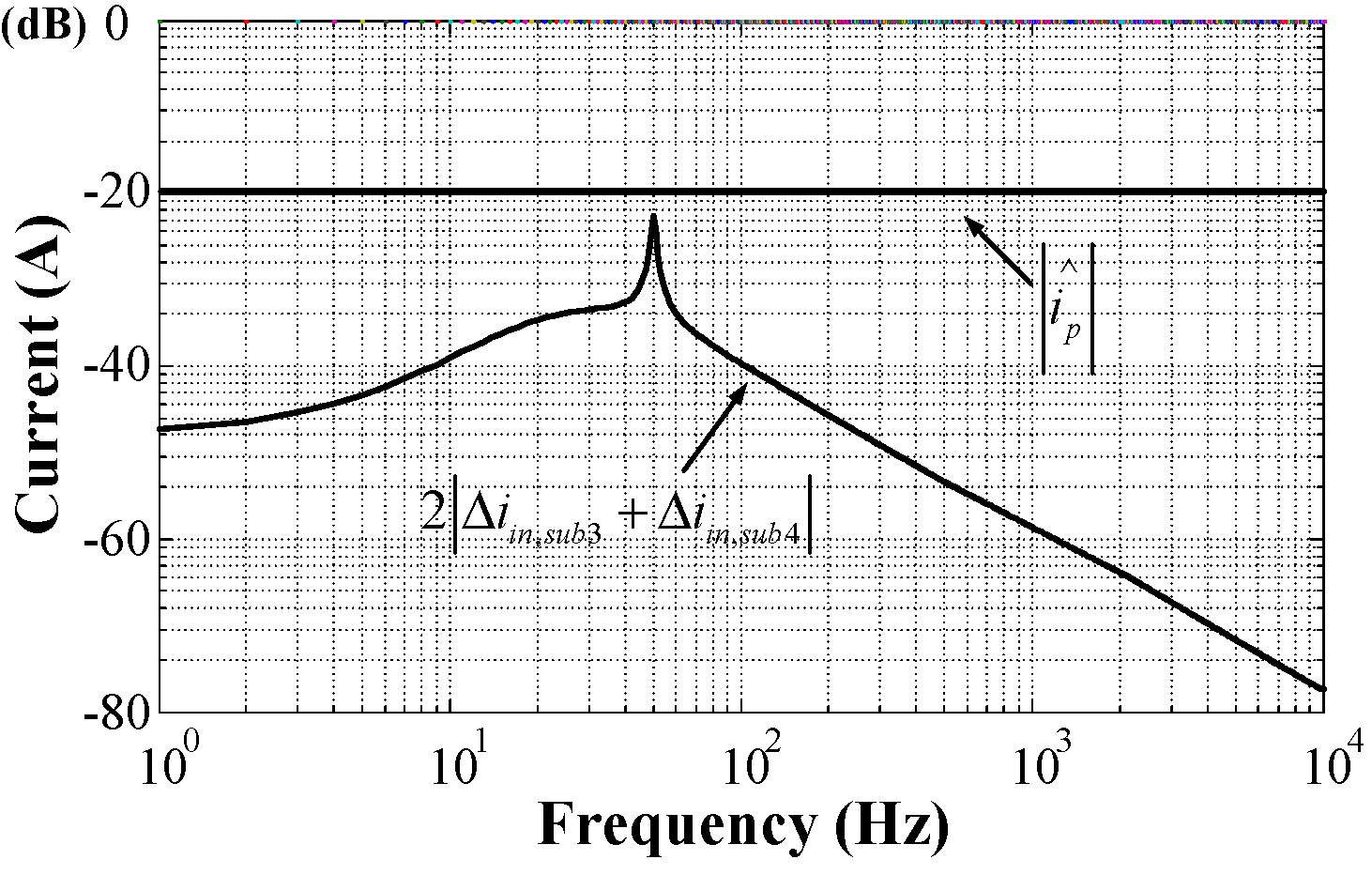
Figure 9.
Relationship between measured currents of and in a stable case.
Figure 9.
Relationship between measured currents of and in a stable case.
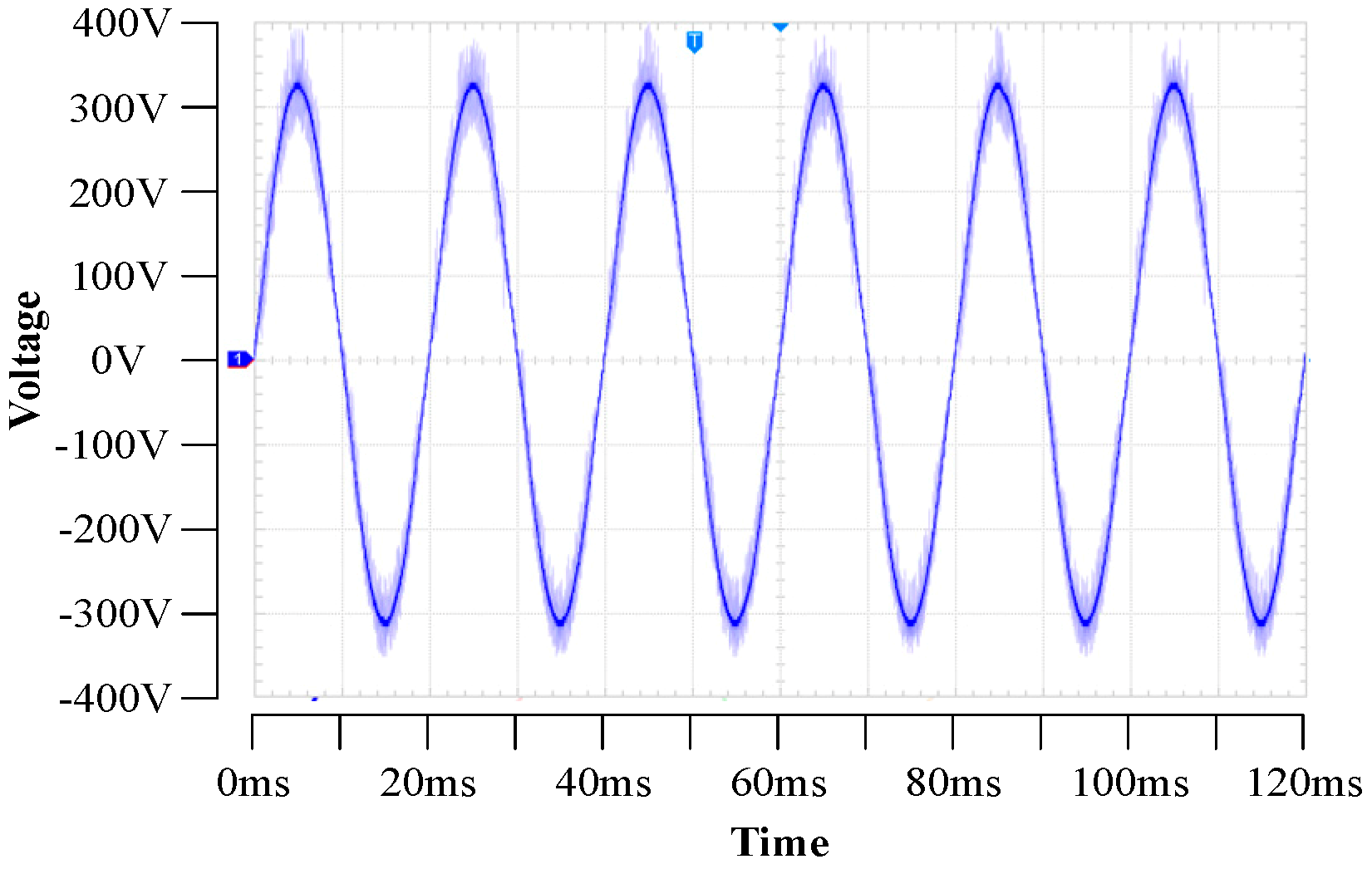
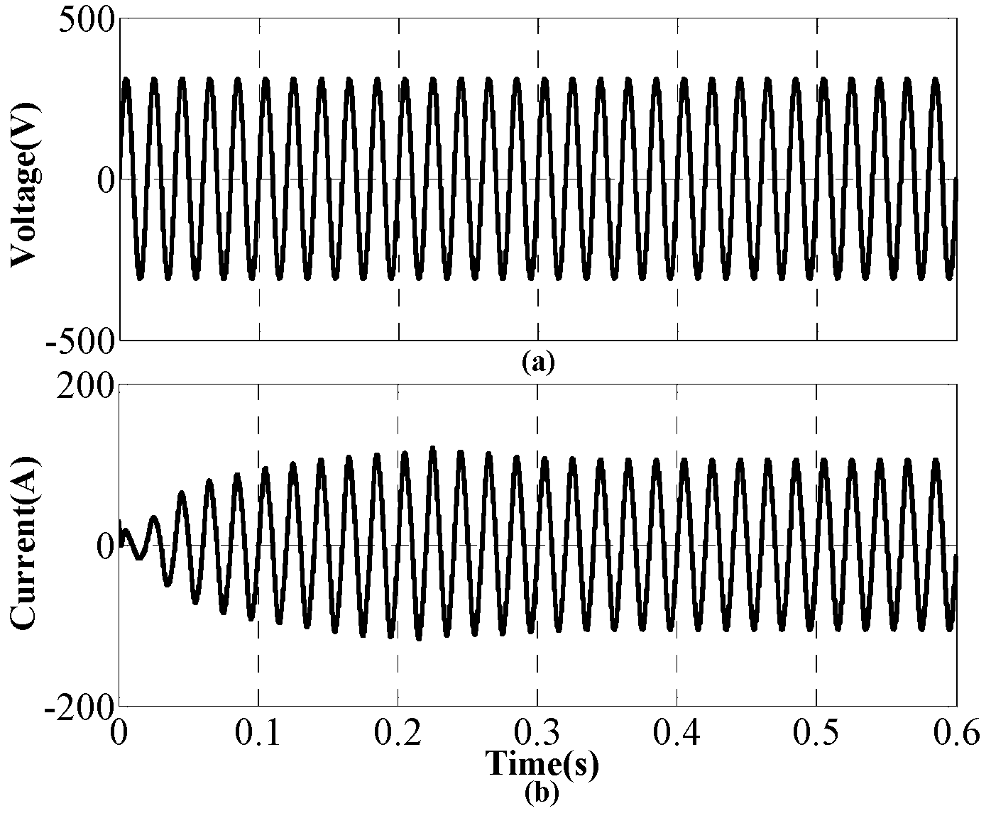
Figure 10.
The input voltage/current of the AC-DC front-end side converter in a stable case.
Figure 10.
The input voltage/current of the AC-DC front-end side converter in a stable case.
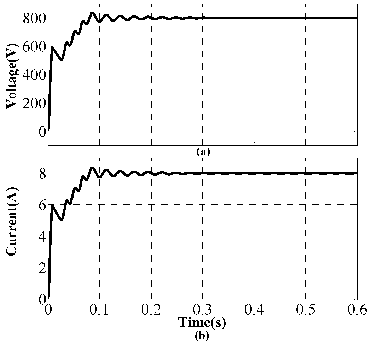
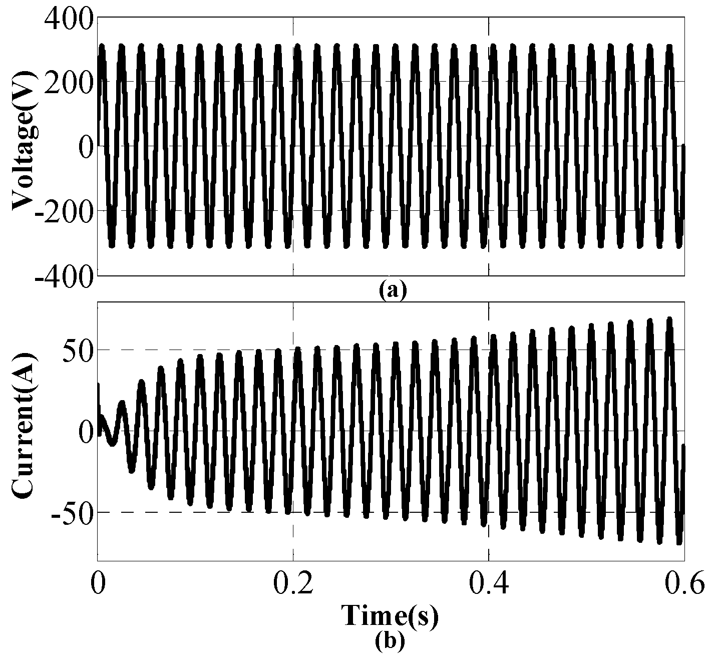
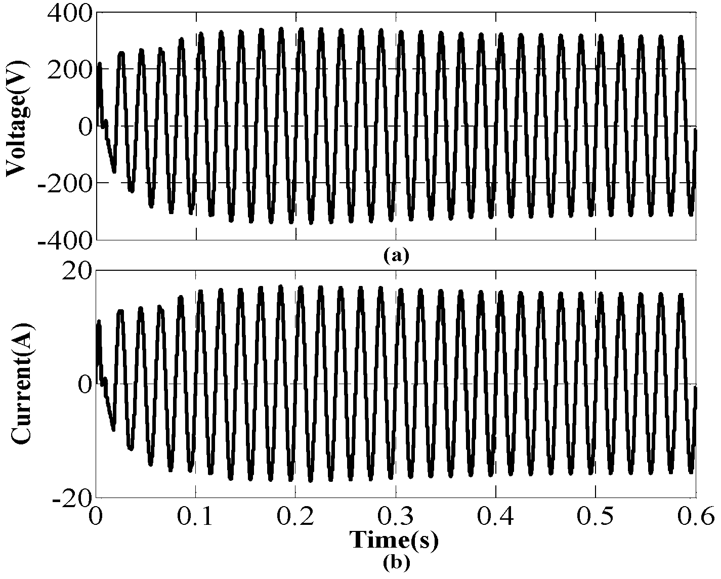
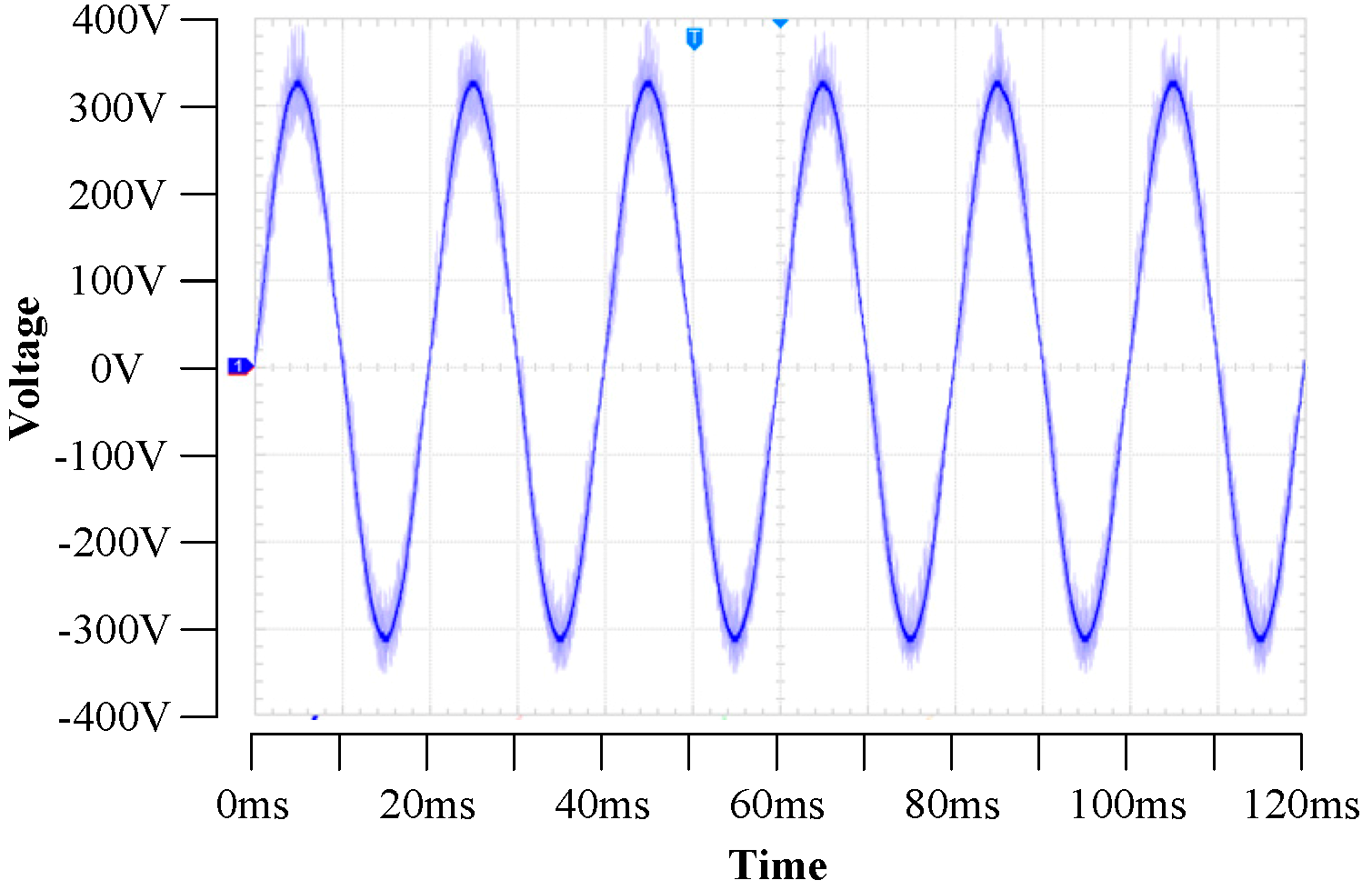
Figure 11.
The output voltage/current of the DC-AC back-end side converter in a stable case.
Figure 11.
The output voltage/current of the DC-AC back-end side converter in a stable case.
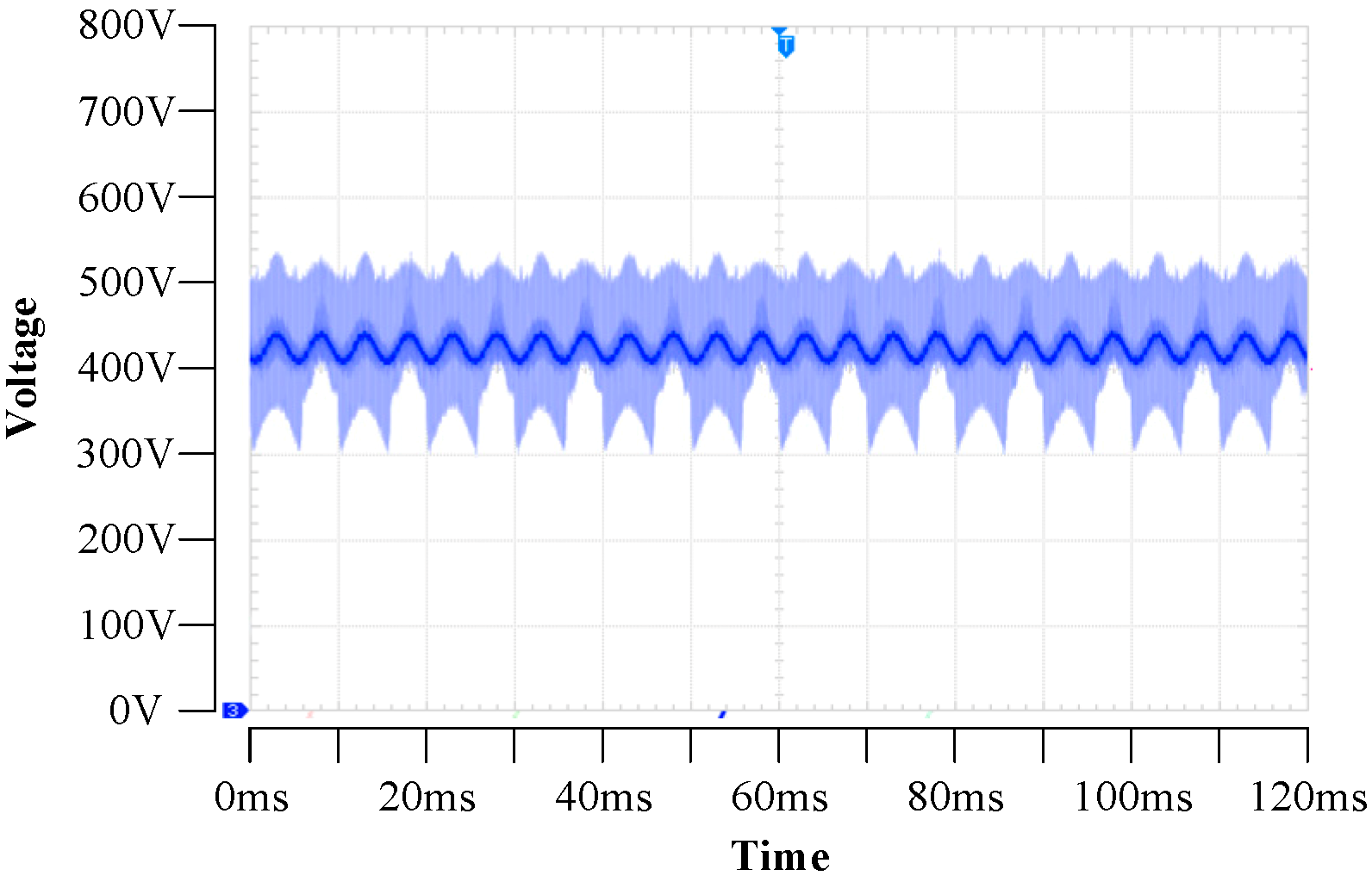
Figure 12.
The output voltage/current of the DC-DC back-end side converter in a stable case.
Figure 12.
The output voltage/current of the DC-DC back-end side converter in a stable case.
Figure 13.
Relationship between measured currents of and in the next steady-state operation point.
Figure 13.
Relationship between measured currents of and in the next steady-state operation point.
Figure 14.
Relationship between measured currents of and in the next steady-state operation point.
Figure 14.
Relationship between measured currents of and in the next steady-state operation point.
Figure 15.
The input voltage/current of the AC-DC front-end side converter in the next steady-state operation point.
Figure 15.
The input voltage/current of the AC-DC front-end side converter in the next steady-state operation point.
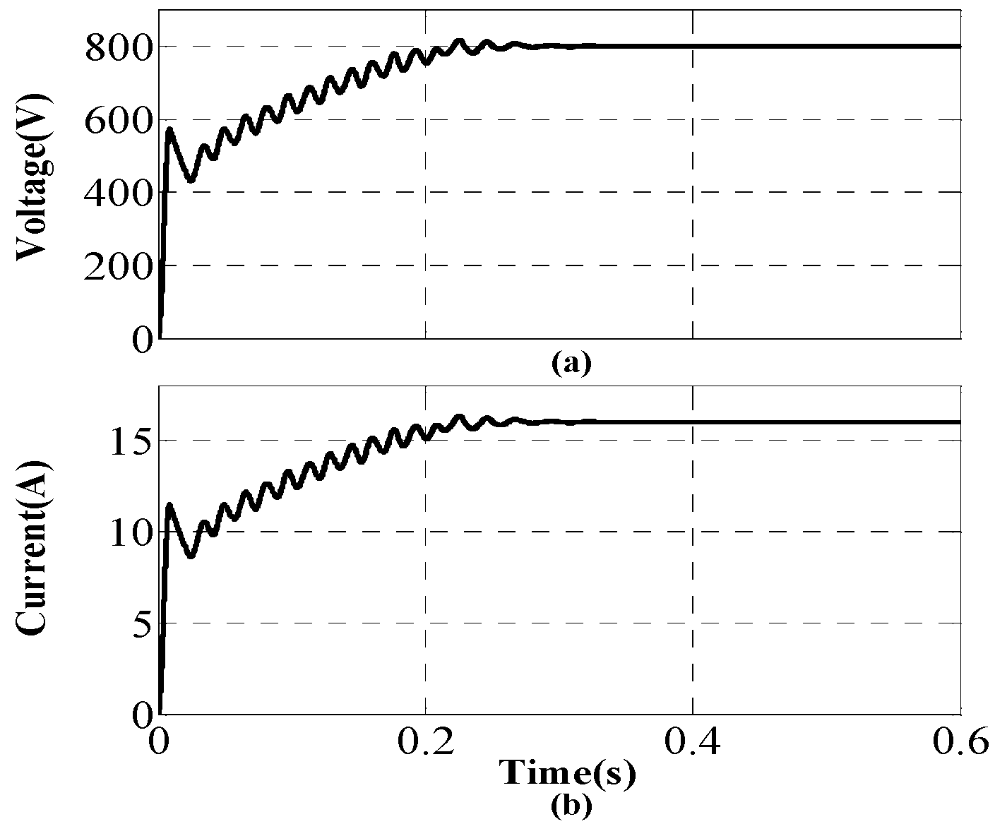
Figure 16.
The output voltage/current of the DC-AC back-end side converter in the next steady-state operation point.
Figure 16.
The output voltage/current of the DC-AC back-end side converter in the next steady-state operation point.
Figure 17.
The output voltage/current of the DC-DC back-end side converter in the next steady-state operation point.
Figure 17.
The output voltage/current of the DC-DC back-end side converter in the next steady-state operation point.
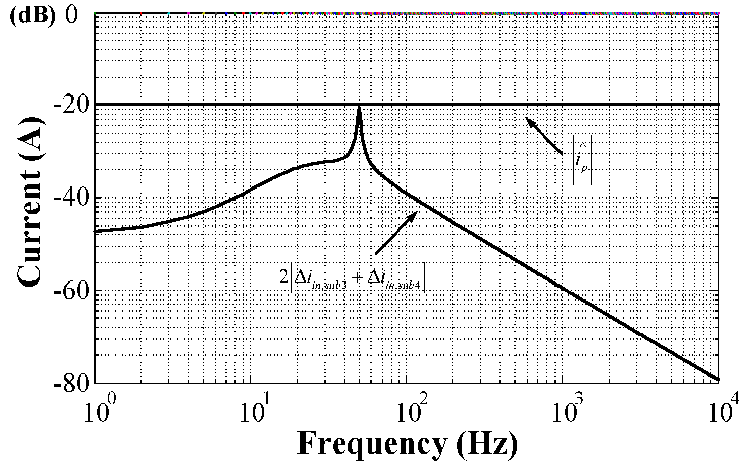
Figure 18.
Relationship between measured currents of and in an unstable case.
Figure 18.
Relationship between measured currents of and in an unstable case.
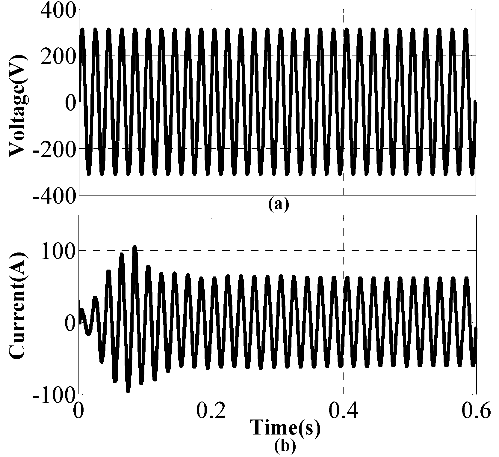
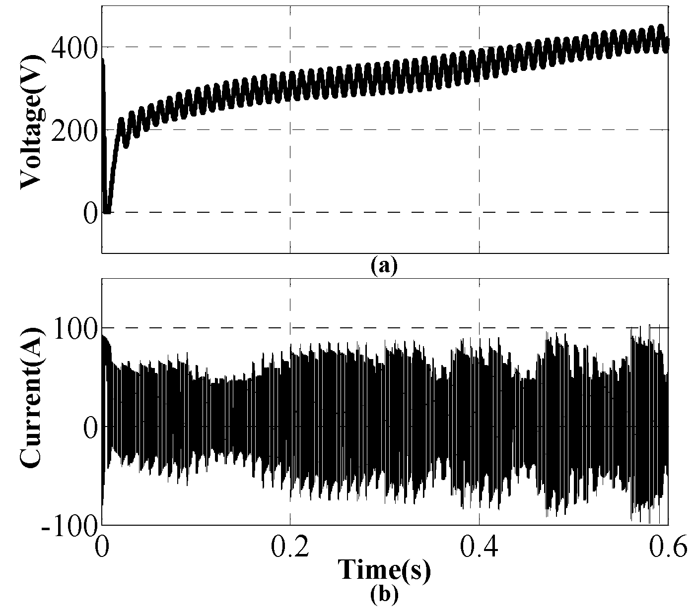
Figure 19.
The input voltage/current of the AC-DC front-end side converter in an unstable case.
Figure 19.
The input voltage/current of the AC-DC front-end side converter in an unstable case.
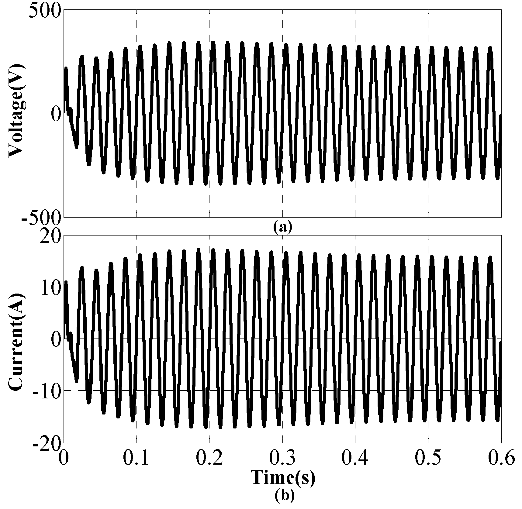
Figure 20.
The output voltage/current of the DAB in an unstable case.
Figure 20.
The output voltage/current of the DAB in an unstable case.
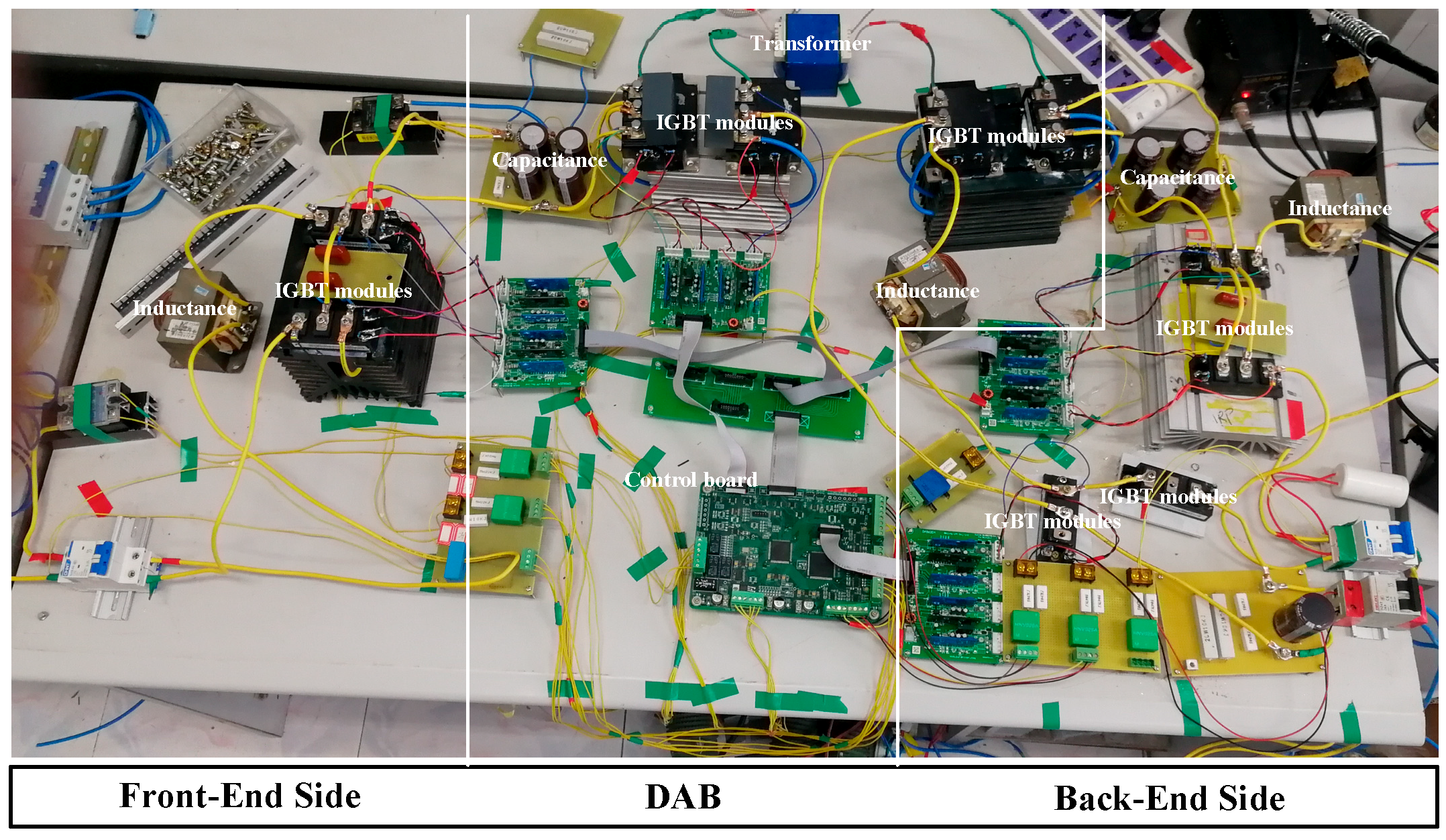
Figure 21.
Experimental hardware test setup.
Figure 21.
Experimental hardware test setup.
Figure 22.
Relationship between measured currents of and in a stable case of the experiment test system.
Figure 22.
Relationship between measured currents of and in a stable case of the experiment test system.
Figure 23.
Relationship between measured currents of and in a stable case of the experiment test system.
Figure 23.
Relationship between measured currents of and in a stable case of the experiment test system.
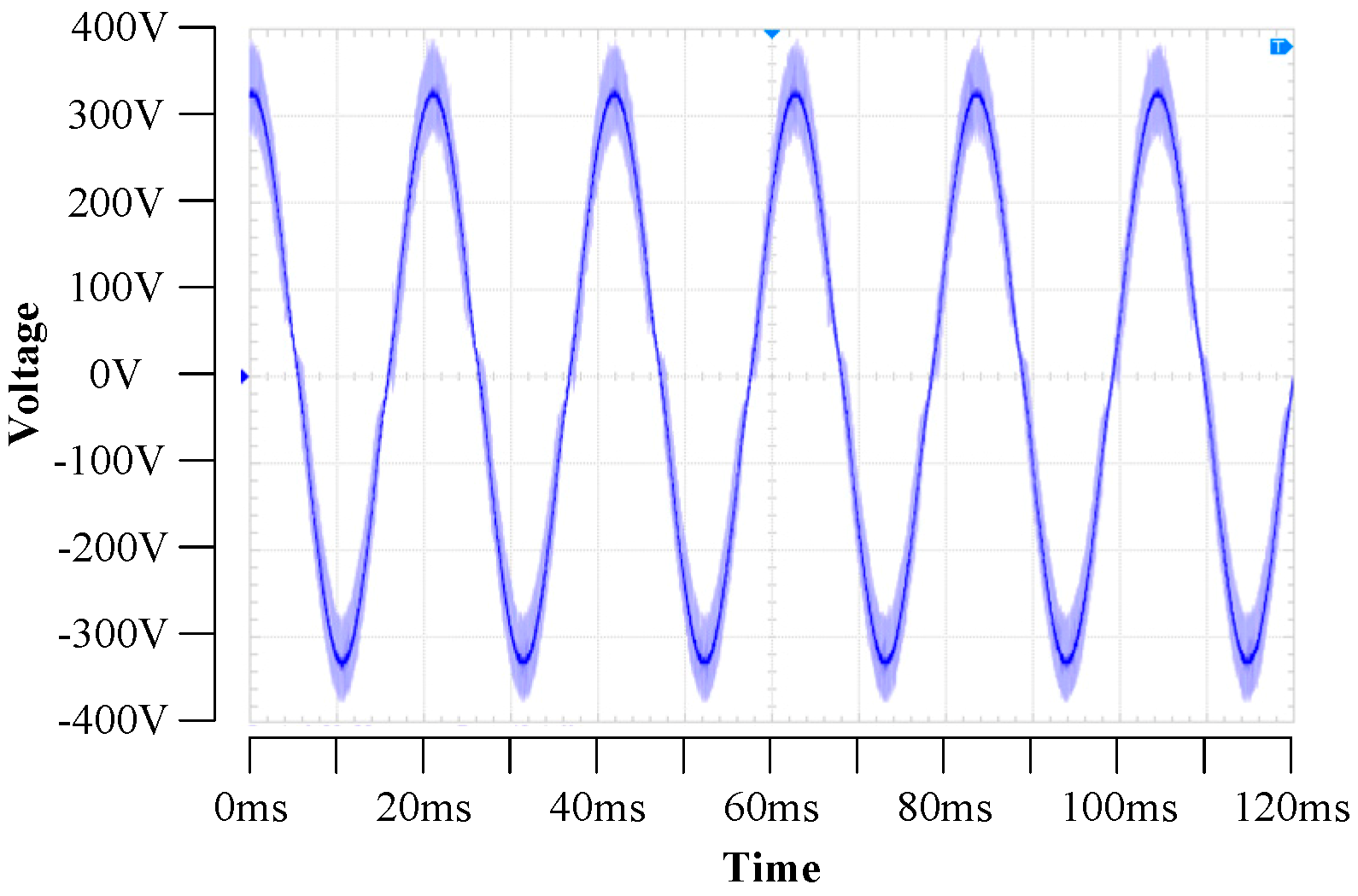
Figure 24.
The input voltage of the AC-DC front-end side converter in a stable case of the experiment test system.
Figure 24.
The input voltage of the AC-DC front-end side converter in a stable case of the experiment test system.
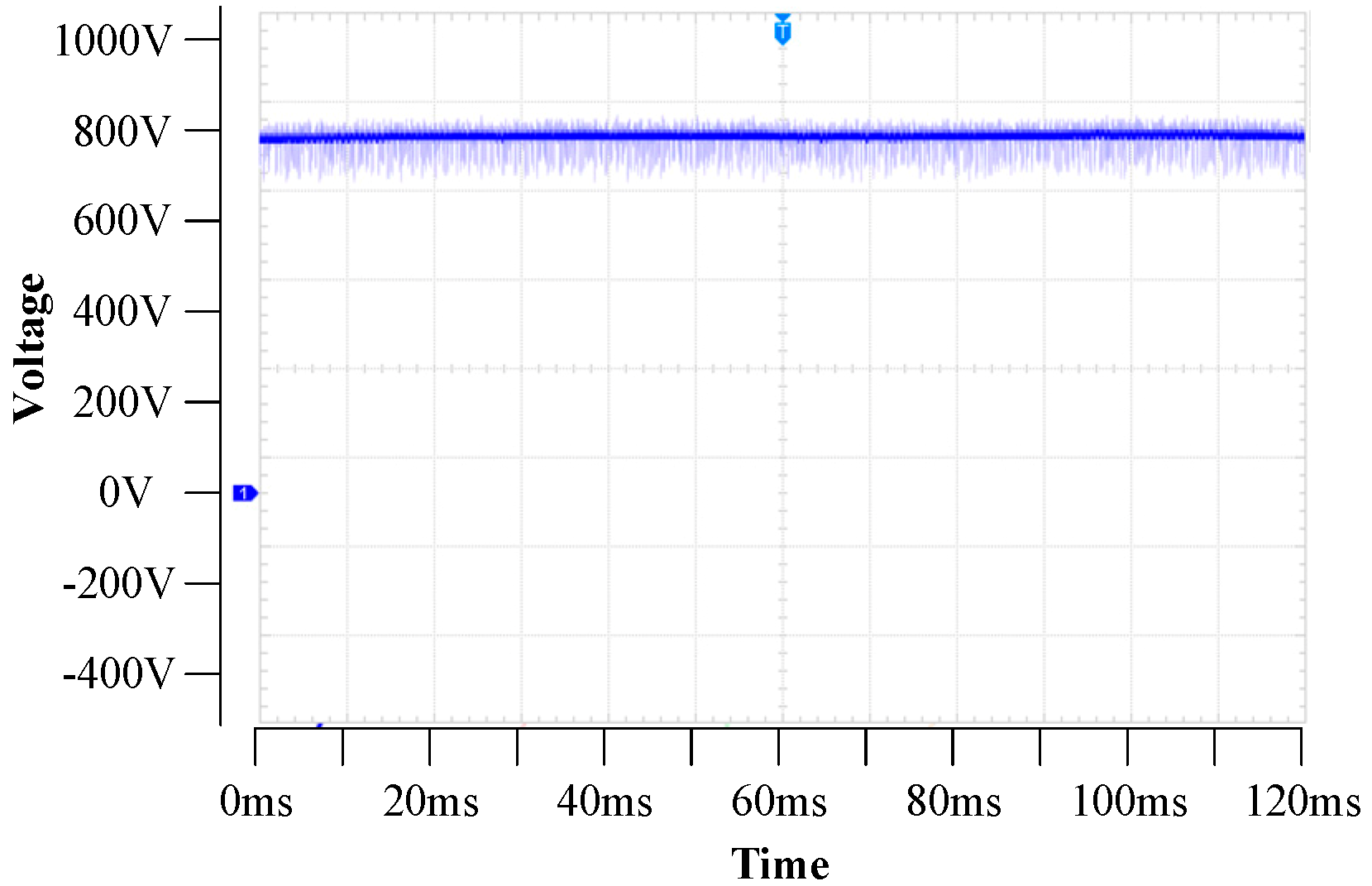
Figure 25.
The output voltage of the DC-AC back-end side converter in a stable case of the experiment test system.
Figure 25.
The output voltage of the DC-AC back-end side converter in a stable case of the experiment test system.
Figure 26.
The output voltage of the DC-DC back-end side converter in a stable case of the experiment test system.
Figure 26.
The output voltage of the DC-DC back-end side converter in a stable case of the experiment test system.
Figure 27.
Relationship between measured currents of and in an unstable case of the experiment test system.
Figure 27.
Relationship between measured currents of and in an unstable case of the experiment test system.
Figure 28.
The input voltage of the AC-DC front-end side converter in an unstable case of the experiment test system.
Figure 28.
The input voltage of the AC-DC front-end side converter in an unstable case of the experiment test system.
Figure 29.
The output voltage of the DAB in an unstable case of the experiment test system.
Figure 29.
The output voltage of the DAB in an unstable case of the experiment test system.
Table 1.
The parameters of the AC-DC front-end side converter.
Table 1.
The parameters of the AC-DC front-end side converter.
| Parameters | Values |
|---|
| |
| |
| |
| |
| |
| |
| |
| |
| 1 |
| |
Table 2.
The parameters of the dual active bridge (DAB).
Table 2.
The parameters of the dual active bridge (DAB).
| Parameters | Values |
|---|
| |
| |
| 0.1875 |
| |
| |
Table 3.
The parameters of the AC-DC front-end side converter.
Table 3.
The parameters of the AC-DC front-end side converter.
| Parameters | Values |
|---|
| |
| |
| |
| |
| |
| |
| 1.286 |
| |
| |
| |
| 0.5 |
Table 4.
The poles of the closed transfer functions.
Table 4.
The poles of the closed transfer functions.
| Poles | Values | Poles | Values |
|---|
| −100.0025 | | −1.8750 |
| −114.7801 | | −409.3200 |
| −2206.5249 | | −10.0008 |
| −9591.9 + j49604 | | −9591.9 − j49604 |
| −47560.9258 | | −18343.1446 |
| −5267.3217 + j14609.2417 | | −5267.3217 − j14609.2417 |
| −168.3590 + j2896.0036 | | −168.3590 − j2896.0036 |
| −0.3333 | | −3.7890 × 10⁻³ |
Table 5.
The experimental parameters of the MS3T.
Table 5.
The experimental parameters of the MS3T.
| Parameters | Values | Parameters | Values |
|---|
| | | |
| | | |
| | | |
| | | |
| | | |
Table 6.
The poles of the experimental text system closed transfer functions.
Table 6.
The poles of the experimental text system closed transfer functions.
| Poles | Values | Poles | Values |
|---|
| −100.0025 | | 1.8750 |
| −114.9710 | | −392.4269 |
| −2757.2272 | | −10.0008 |
| −9592 + j49604 | | −95912 − j49604 |
| −48634.9072 | | −19044.1187 |
| −4510.6015 + j16665.5791 | | −4510.6015 − j16665.5791 |
| −39.4247 + j1187.1495 | | −39.4247 − j1187.1495 |
| −0.3333 | | −3.7890 × 10⁻³ |


