CO₂ Pipeline Design: A Review

Abstract

There is a need to accurately design pipelines to meet the expected increase in the construction of carbon dioxide (CO₂) pipelines after the signing of the Paris Climate Agreement. CO₂ pipelines are usually designed with the assumption of a pure CO₂ fluid, even though it usually contains impurities, which affect the critical pressure, critical temperature, phase behaviour, and pressure and temperature changes in the pipeline. The design of CO₂ pipelines and the calculation of process parameters and fluid properties is not quite accurate with the assumption of pure CO₂ fluids. This paper reviews the design of rich CO₂ pipelines including pipeline route selection, length and right of way, fluid flow rates and velocities, need for single point-to-point or trunk pipelines, pipeline operating pressures and temperatures, pipeline wall thickness, fluid stream composition, fluid phases, and pipeline diameter and pressure drop calculations. The performance of a hypothetical pipeline was simulated using gPROMS (ver. 4.2.0) and Aspen HYSYS (ver.10.1) and the results of both software were compared to validate equations. Pressure loss due to fluid acceleration was ignored in the development of the diameter/pressure drop equations. Work is ongoing to incorporate fluid acceleration effect and the effects of impurities to improve the current models.

1. Introduction

Greenhouse gases are mainly responsible for the gradual rise in atmospheric temperatures. One of the chief components of greenhouse gases is carbon dioxide (CO₂). CO₂ is released from many natural and anthropogenic processes including power generation, gas-flaring, breathing, automobiles, volcanic eruptions, etc. Of these, the anthropogenic release of CO₂ is of concern and the need to reduce the percentage of CO₂ in the atmosphere becomes pertinent due to the adverse effects on the environment. According to the Intergovernmental Panel on Climate Change (IPCC) [1], global warming for the past 50 years is mostly due to the burning of fossil fuels. In 2010, CO₂ emissions amounted to about 37 Gt representing about 72% out of 51 Gt of greenhouse gas emissions [2]. About three-fourths of atmospheric CO₂ rise is because of burning fossil fuels [3], which releases CO₂ into the atmosphere. If this unchecked release of CO₂ into the atmosphere continues, temperatures are expected to increase by about 6.4 °C by year 2100 [4] with attendant rises in sea level.

CO₂ capture and storage (CCS) seeks to capture CO₂ from large emission sources and safely store it in underground reservoirs or use it for Enhanced Oil Recovery (EOR) operations [5]. CCS is a relatively advanced technology seeking to capture anthropogenic CO₂ and reduce emissions to attain less than 2 °C increase (as proposed in the Paris agreement) of pre-industrial Earth temperatures [6,7]. Mazzoccoli et al. [8] and IPCC [9] reported that CO₂ releases into the atmosphere must be less than 85% by 2050 compared to year 2000 levels to achieve not more than 2.4 °C increase in atmospheric temperature. This seems like an ambitious target considering the level of implementation of CCS across the globe.

More CO₂ is expected to be generated as more places become industrialised. The demand for CO₂ is only a small fraction of the quantity generated in industrial processes. The highest demand for CO₂ is in EOR with pipelines transporting it, mainly in the USA and Canada. For example, the Alberta Carbon Trunk Line (ACTL) is designed to transport about 5000 tonnes of CO₂ per day from industrial sources to an EOR field where it will be used to unlock light oil reserves from reservoirs depleted from primary production [10]. The demand for CO₂ for increased EOR operations would peak about the year 2025, requiring the transportation of about 150 million tons of CO₂ [11]. This is a small fraction of the over 6870 million metric tons of greenhouse gas emissions in the USA alone in 2014 [12].

Transportation is the link between CO₂ capture and storage. CCTS, which stands for CO₂ capture, transportation and storage [13], is occasionally used interchangeably with CCS. Although transportation may be the lowest cost intensive part of the CCS process, it may be the most demanding when it comes to planning and guidance [14]. Pipelines, railcars and tanker trucks can transport CO₂ on land while offshore transportation involves ships and pipelines [15]. The efficient transportation of CO₂ from source to sink requires the adequate design of pipelines for CO₂ transportation [16].

Before CO₂ is transported, it is captured from the flue gas of industrial processes or natural sources and purified. Capture is the most cost intensive component of the CCS chain, accounting for about 50% [17] and with compression cost, up to 90% [18] of total CCS cost. After transporting the CO₂ to the storage site, it is stored in depleted oil and gas fields or saline aquifers [19]. There seems to be enough storage locations in the world. The UK alone has CO₂ storage capacity of about 78 Gt in saline aquifers [20]. This means that there is enough storage capacity to store all the CO₂ captured, but because the capture sites may not be close to the storage sites, it needs to be transportated.

In designing a CO₂ pipeline, consideration is given to pipeline integrity, flow assurance, operation and health/safety issues [21]. CO₂ pipeline design relies heavily on the thermo-physical properties of the flowing fluid. Though the behaviour of CO₂ in various phases have been studied, the high pressure and varying temperature of CO₂ fluids and the impurities in the fluid make them difficult to predict [21,22]. Therefore, the need to study specific pipelines and design them for low cost, good performance and safe operation is important [22]. Three stages of pipeline operations were identified including: design, construction and operations [23]. This review focusses on the first part; design of CO₂ pipelines. There are existing regulations and standards, which guide the design of pipelines. These include, wall thickness, over-pressure protection systems, corrosion protection, protection from damage, monitoring and safety, access routes, etc. [23]. What is considered in CO₂ pipeline design also depends on different operating conditions including operating pressures (maximum and minimum), temperature, fluid composition, pipeline corrosion rate, ambient temperatures, CO₂ dehydration, topography of the pipeline route (changes in elevation and pipeline bends), compressor requirements, joint seals, transient flow minimisation, impact of CO₂ release on human health, etc. [24]. A minimum consideration for CO₂ pipeline design should include determining physical properties of the flowing fluid, optimal pipeline sizes, specification of operating pressures of the pipeline, adequate knowledge of the topography of the pipeline route, geotechnical considerations and the local environment [21].

This literature review focuses mainly on available models of pipeline pressure drop and pipeline diameter calculations. These two interdependent parameters and the fluid flow rate are the most important parameters in the process design of CO₂ pipelines. This review concentrates on pipeline diameter estimation and/or pressure drop prediction. First, some existing CO₂ pipelines in the world are listed followed by a review of the important factors affecting pipeline design. These include: pipeline route, length and right of way (ROW), CO₂ flow rates and velocity, point-to-point (PTP) and trunk/oversized pipelines (TP/OS), CO₂ pipeline operating pressures and temperatures, pipeline wall thickness, CO₂ composition, possible phases of CO₂ in pipelines and finally models for determining pipeline diameter and pressure drop. Finally, it discusses the performance of the available diameter determination models.

2. Existing CO₂ Pipelines

Presently, there is a combined total of over 8000 km of CO₂ pipelines around the world. This is up from over 6500 km of CO₂ pipelines in 2014 [25], and from 2400 km in 2007 [26]. According to Chandel et al. [27], the US had over 3900 km of pipelines in 2010 transporting 30 million tonnes (Mt) of CO₂ annually [28]. The total length of CO₂ pipelines in the US increased to over 6500 km in 2014 [29]. By 2015, there were 50 individual CO₂ pipelines in the US with a total length of 7200 km [30]. Europe had only about 500 km of CO₂ pipelines in 2013 [31]. Over 200,000 km of pipelines would be required to transport about 10 billion tonnes (Gt) yearly from the year 2050. If the Paris Agreement is taken seriously, the implementation of CCS in many countries shall increase.

Table 1. Existing and planned CO₂ pipeline projects [25,33,34,35].

Pipeline Name	Length (km)	Capacity (Mt/y)	Diameter (mm)	Status	Country
Quest	84	1.2	324	Planned	Canada
Alberta Trunkline	240	15	406	Planned	Canada
Weyburn	330	2.0	305–356	Operational	Canada
Saskpower Boundary Dam	66	1.2		Planned	Canada
Beaver Creek	76		457	Operational	USA
Monell	52.6	1.6	203	Operational	USA
Bairoil	258	23		Operational	USA
West Texas	204	1.9	203–305	Operational	USA
Transpetco	193	7.3	324	Operational	USA
Salt Creek	201	4.3		Operational	USA
Sheep Mountain	656	11	610	Operational	USA
Val verde	130	2.5		Operational	USA
Slaughter	56	2.6	305	Operational	USA
Cortez	808	24	762	Operational	USA
Central Basin	231.75	27	406	Operational	USA
Canyon Reef Carriers	225		324–420	Operational	USA
Chowtaw (NEJD)	294	7	508	Operational	USA
Decatur	1.9	1.1		Operational	USA
Snohvit	153	0.7		Operational	Norway
Peterhead a	116	10		Cancelled	UK
White Rose a	165	20		Cancelled	UK
ROAD a	25	5	450	Cancelled	The Netherlands
OCAP	97	0.4		Operational	The Netherlands
Lacq	27	0.06	203–305	Operational	France
Rhourde Nouss-Quartzites	30	0.5		Planned	Algeria
Qinshui	116	0.5	152	Planned	China
Gorgon	8.4	4	269–319	Planned	Australia
Bravo	350	7.3	510	Operational	USA
Bati Raman	90	1.1		Operational	Turkey
SACROC	354	4.2	406	operational	USA
Este	191	4.8	305–356	Operational	USA

^a Reported as planned but now cancelled.

shows some existing and planned CO₂ pipelines in the world. The Peterhead and White Rose projects were reported as planned but both projects have now been cancelled. The £1 billion CCS Competition was cancelled by the UK government on 25th of November 2015, prior to awarding the contracts for both the Peterhead and the White Rose CCS projects [32].

3. Pipeline Route, Length and Right of Way (RoW)

Determining the pipeline route and length is the first thing to consider in the design of pipelines. Siting a pipeline involves determining, assessing and evaluating alternative routes and acquiring the Right of Way (ROW) of a selected route [36]. This route is the optimum path, which may not necessarily be the shortest path that connects the source of CO₂ to the sink. This route ultimately determines the length of the pipeline. Many factors are considered while planning the route of a CO₂ pipeline including safety and running the pipeline across uninhabited areas [37]. The aim of designing an optimum route is to reduce the pipeline length, reduce cost by using existing infrastructure, avoid roads, rails, hills, lakes, rivers, orchards, water crossings and inhabited areas, minimise ecological damage, and have easy access to the pipeline [38].

A straight path for pipelines from source to sink is rarely achieved as obstacles such as cities, railways, roads, archaeological sites or sensitive natural resources or reserves may be in the way, which have to be avoided [25]. In most cases, avoiding these obstacles increase the length of the pipeline resulting to increased capital and operational costs. While planning for the route, sometimes as many as twenty possible routes may be developed in the planning stage, e.g., as in the Peterhead CCS project in the UK [25] and the optimum route selected.

The pipeline route will determine the total length of the pipeline and the bends on it. The pipeline route thus controls the cost of pipeline transport as it affects the length, material, number and degree of bends and the number of booster stations to be installed [39,40]. Even the pipeline pressure drop is dependent among other factors on the length of the pipeline [41]. The pressure drop along a pipeline would be greater for longer pipelines than for shorter ones with similar characteristics. Gao et al. [40] concluded that longer pipelines also require larger pipeline diameters thereby increasing the capital and levelised costs. It is therefore desirable to reduce the length of the pipeline as much as possible but this is constrained by the requirements for an optimum route. The route selection is an economic decision and the optimum route is the cheapest path in terms of capital, operational and maintenance costs.

After identifying the path or route of the pipeline and before doing any work, the route is acquired. The document detailing the route for the pipeline, referred to as right of way (ROW) has to be secured with negotiations with the legal owners which might include federal, state, county, other governmental agencies or private owners [38]. It is necessary to have several routes in order of preference because inability to secure a ROW can cause the route to be changed. In order to avoid delays in the execution of the project, it is necessary to investigate and determine the right authorities and people to apply to and obtain all local permits to enable free access to work on the route of the pipeline [42]. Some of the items to be identified and permit sought include; roadways, railroads, canals, ditches, overhead power lines, underground pipelines and underground cables [42]. These obstacles inevitably increase the cost of constructing a CO₂ pipeline. Work can only commence after the ROW document is acquired legally. The ROW document is not always easy to acquire and it could account for 5% [31], between 4% and 9% [43] or between 10% and 25% [44] of the total pipeline construction cost. Pipeline ROW is generally easier to obtain in rural areas than in urban areas [45], because in rural areas, the pipeline crosses less developed land with fewer infrastructure.

4. Pipeline CO₂ Flow Rates and Velocity

Flow rate indicates the volume of fluid transported from source to sink and it determines the minimum pipeline diameter that would be adequate for transportation. A pipeline diameter that is too small for the flow rate would cause high velocity of the fluid with attendant high losses in pressure and erosion of the pipe wall. Flow rate is measured in either mass or volume units. Equation (1) shows a simple relationship between the two units of measurement:

$$Q=Q_v\times \rho$$

(1)

where Q = flow rate (kg/s), Q_v = flow rate (m³/s) and ρ is density (kg/m³).

Flow rate if unchanged, determines the optimal diameter of the pipeline [46]. Pipeline diameter must not be too large to avoid excessive pipeline cost yet not too small to cause high velocities and pressure losses. Even pipelines with very small diameter can be used to transport high flow rates. However, these pipelines would have very high velocities, high pressure losses, noise and erosion of the internal pipeline wall. Very large pipeline diameters would reduce pressure losses, have low velocities and low or non-existent noise and erosion, but these are very expensive. The optimum diameter should therefore be large enough to avoid high pressure losses, high erosion and noise but not too expensive. There may be a need to construct an oversized pipeline where two sources of CO₂ occur in close proximity but are not available for transportation at the same time but can be considered for future expansion projects. The cost of constructing a new pipeline when the second source comes on stream is avoided but the initial pipeline cost is increased. The diameter of the oversized pipeline may not be optimum for either the initial flow rate or the final flow rate. Operational and economic factors determine the appropriate oversized diameter size. Wang et al. [46] stated that the relationship between diameter ratio and flow rate ratio was linear and that for a tripling of flow rate, the optimal diameter was about 4.2 times larger. Diameter values in Bock et al. [47] and Equation 20 (described in Section 10), used to simulate pipeline diameter while holding pressure drop and length of pipeline constant gave similar values. Figure 1 shows the linear relationship between diameter ratio and flow rate ratio but a threefold increase in flow rate only resulted to an increase in the diameter size by about 1.6 times.

Gao et al. [40] concluded that a higher mass flow rate increases the pipeline diameter, which in turn increases the pipeline capital cost. Some cost models based the investment cost equation only on CO₂ flow rate and length of pipeline [48,49]. The flow velocity in the pipeline is calculated using Equation (2) [27,50]:

$$v=\frac{Q_v}{A}=\frac{4Q}{\rho \pi D^2}$$

(2)

where v = velocity (m/s), D = pipeline internal diameter (m), A = cross-sectional area of pipeline (m²).

It is impossible to have a conceptual design of CO₂ pipelines without adequate knowledge of expected fluid flow rate. The flow rate of the CO₂ fluid is therefore the most important parameter in the design of CO₂ pipelines. It is important to establish the maximum velocity or erosional velocity in the pipeline to avoid rapid erosion of the inner pipeline wall and/or high pressure losses [51]. American Petroleum Institute (API) [52] presented an empirical formula to calculate erosional velocity for two-phase flow (Equation (3)). Pipeline diameter is selected to limit the velocity of CO₂ fluid to below the erosional velocity and avoid excessive pressure losses. Vandeginste and Piessens [39] applied the API-RP-14E formula (Equation (3)) to calculate erosional velocity and arrive at an erosional velocity of 4.3 m/s, which is higher than 2.0 m/s widely used. A similar equation used to specify the maximum velocity to avoid noise and erosion according to API standard [53], is given in Equation (4). Velocity values computed with Equation (4) are higher than values computed with Equation (3). The expected CO₂ flow rate is ascertained and an erosional velocity is calculated for the pipeline. With an assumed velocity less than the erosional velocity and considering pressure losses, an adequate internal pipeline diameter is determined. An additional pipeline is considered where the flow rate is too high for a single pipeline:

$$v_e=0.82\frac{c}{\sqrt{\rho }}$$

(3)

where v_e = erosional velocity (m/s) and c = empirical constant (100 for continuous flow and 125 for intermittent flow):

$$v_{max}=\frac{122}{\sqrt{\rho }}$$

(4)

where v_max = maximum velocity (m/s).

5. Consideration for Point-to-Point (PTP) or Trunk/Oversized Pipelines (TP/OS)

After ascertaining the flow rate of CO₂, it may be necessary to decide whether to design a trunk line or “point-to-point” pipelines where more than one CO₂ source exist in close proximity. A trunk pipeline also called a backbone or oversized pipeline connects two or more pipelines from CO₂ sources to a single sink or multiple sinks while point-to-point (PTP) direct pipelines connect single CO₂ sources to single sink(s). The decision to construct a trunk pipeline or single PTP pipelines is purely economic. Knoope et al. 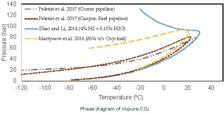[54] and the Intergovernmental Energy Agency for Greenhouse Gas Research and Development Programme IEA GHG [55] concluded that a point-to-point connection is more cost effective if two sources are 100 km from a sink and the angle made by imaginary straight lines joining the two sources to the single sink is greater than 60°. Three scenarios (“point-to-point”, “tree and branches” and “hub and spoke”) of two sources and one sink, with varying angles made by straight lines joining the two sources to the sink from 0° to 120°. The cost of the pipeline was modelled at $50,000 per km per inch and the annual OPEX was assumed at 5% of CAPEX. It was concluded from the analysis that for angles greater than 90°, no cost saving was achieved by the use of a trunk pipeline. For angles between 30° and 60°, the “radial hub and spoke” scenario appeared to be the optimum option and below 15°, the “tree and branches” scenario gave the lowest cost.

Table 2. Length of pipelines (km).

Angles (degrees)	Tree and Branch (km)		Hub and Spoke (km)
	A/B	Trunk	A/B	Trunk
10	8.72	99.62	50.19	50.19
20	17.36	98.48	50.77	50.77
30	25.88	96.59	51.76	51.76
45	38.27	92.39	54.12	54.12
60	50.00	86.60	57.74	57.74
90	70.71	70.71	70.71	70.71
120	86.60	50.00	86.60	50.00

shows the lengths of the three pipelines when varying the angles that straight lines from the two sources make at the single sink between 10° and 120°. The distance of each of the two sources from the sink is held constant at 100 km. The length of the trunk pipeline decreases for the “tree and branch” arrangement but increases for the hub and spoke arrangement as the angle made by straight lines drawn from the two sources to the sink increases. A single trunk pipeline is considered only where the two sources occur at close proximity with negligible distance between them, assumed to form 0 degrees at the sink. Figure 2 shows the capital cost profile of the three pipeline scenarios (two single pipelines, (A and B), and one trunk pipeline), assuming $50,000 per km per inch. The “hub and spoke” arrangement becomes a “tree and branch” arrange for angles greater than 90° because the three pipelines can no longer have equal lengths. Between 24° and 90°, the “hub and spoke” arrangement is more cost effective than the “tree and branch” arrangement. Greater than 47° for the “tree and branch” and greater than 67° for the “hub and spoke” arrangements, the single pipelines are cheaper, respectively. Below 24° the “tree and branch” arrangement is cheaper than the “hub and spoke” arrangement.

Wang et al. [56] presented Equation (5) to calculate the trade-off point between the use of a trunk pipeline and single point-to-point separate pipelines that transport CO₂ from two sources starting production at different times. The trade-off point does not depend on the length of the pipeline if the pipeline length is less than or equal to 150 km (Equation (5a)). Where the pipeline length is more than 150 km, the trade of point depends also on the length of the pipeline (Equation (5b)). It is however, unclear if this is irrespective of the pipeline diameter. The authors also stated that if the trade-off point and actual time lapse between the two projects are the same (N = N*), then the relationship between the diameter ratio, $D_t/D_1$ and the flow rate ratio $Q_t/Q_1$ is linear (Equation (6)):

$$N_{base}^{*}=\{\begin{array}{c}14.3-0.57Q_1-0.89(Q_t/Q_1), \le 150 \mathrm{km} \left(\mathrm{a}\right)\\ \left(15.1-0.605Q_1\right)e^{-0.00036 L}-0.91(Q_t/Q_1), >150 \mathrm{km} \left(\mathrm{b}\right)\end{array}$$

(5)

$$D_t/D_1=0.22(Q_t/Q_1)+0.7$$

(6)

N*_base = trade-off point (years) or number of years after which duplicate pipelines become more cost effective (base emphasizing assumptions used in the calculations). $D_t$ = oversized pipeline diameter (mm), $D_1$ = diameter of initial duplicate pipeline (mm) Q₁ and $Q_t$ = initial and total flow rate respectively (Mt/y).

If both flows, Q₁ and Q₂ start at the same time, the actual pipeline diameter can be calculated using Equation (7), assuming a hypothetical initial flow rate, i.e., of one pipeline. Equation (7) is in line with results obtained with Bock et al. [47], i.e., Equations (17) and (20) plotted in Figure 1. For a fixed total flow rate (Q_t), the optimum diameter, D_t should be the same irrespective of the initial flow rate but Equation (7) gives increasing values of D_t with increasing Q₁. Equation (8) calculates the optimum oversized pipeline diameter, taking into account the time lapse between the two sources coming on stream and the length of the pipeline:

$$D_t= D_1{\left(Q_t/Q_1\right)}^{0.39}$$

(7)

$$\frac{D_t}{D_1}=\left[1-0.78\left(\frac{N}{N^{*}}\right)\right] {\left(Q_t/Q_1\right)}^{0.39+0.61{\left(\raisebox{1ex}{$N$}\!\left/ \!\raisebox{-1ex}{$N^{*}$}\right.\right)}^{2.1}}+0.7{\left(\raisebox{1ex}{$N$}\!\left/ \!\raisebox{-1ex}{$N^{*}$}\right.\right)}^{0.53}$$

(8)

where N = actual time difference between the two CO₂ sources (years), $D_1$ = optimal diameter for Q₁ (m) and $D_t$ = oversized pipeline diameter (m), Q₁ and Q_t = initial and final flowrates (kg/s).

6. CO₂ Pipeline Operating Pressures and Temperatures

The maximum operating pressure of a CO₂ pipeline is determined by economic considerations. CO₂ can be transported under low pressures (gas phase) or high pressures (dense phase). The minimum pressure is a function of differential pressure requirement for flow to occur and the need to avoid CO₂ phase changes. The upper limit of pipeline pressure is set by economic concerns and ASME-ANSI 900# flange rating and the lower pressure limit is set by supercritical requirement and the phase behaviour of CO₂ [36]. An input (or maximum) pressure and a minimum pressure are used to calculate pressure-boosting distances. Within this distance, the CO₂ remains in the desired fluid phase. The phase behaviour of CO₂ fluids also depend on the temperature of the fluid. There may be significant temperature and pressure changes along long distance pipelines due to frictional pressure loss, expansion work done by the fluid and heat exchange with surroundings [57]. Nimtz et al. [58] stated that pipe wall thickness and existing compressor power (assumed maximum is 20 MPa) restricts the maximum allowable pressure. Another limiting factor for maximum pressure is costs because thick walled pipes are more expensive than thinner walled pipes.

The compressor discharge temperature sets the upper temperature and the ground/environmental temperature sets the lower temperature of pipelines [36]. Typical CO₂ pipeline operating pressures range from 10 to 15 MPa and temperatures from 15 to 30 °C [59] or 8.5 to 15 MPa and 13 to 44 °C [17]. Stipulating minimum pipeline pressure above 7.38 MPa, the critical pressure of CO₂, ensures that the CO₂ fluid remains in the supercritical state [60]. Witkowski et al. [37] raised the pressure to a safe 8.6 MPa to avoid high compressibility variations and changes in specific heat along the pipeline due to changes in temperature. All common impurities studied in Peletiri et al. [61] were found to increase the critical pressure of CO₂ streams above 7.38 MPa and except for H₂S and SO₂, reduce the critical temperature below 30.95 °C. There are slight differences in the pressure ranges reported in the literature, but all pressures are above the critical value of 7.38 MPa. CO₂ pipeline temperatures in Patchigolla and Oakey [59] is below the critical temperature of CO₂. This means that the CO₂ fluid is in the dense (liquid) state and not the supercritical state. The upper temperature reported by Kang et al. [17] is above the critical temperature but the lower temperature is less than the critical value. In this case, the CO₂ fluid may change phase from supercritical state to liquid state along the pipeline.

Pressures are non-linear along a CO₂ pipeline, therefore simple averaging of inlet and outlet pressures may not yield accurate average pressure values. Due to this non-linearity of pressures along a CO₂ pipeline, McCoy and Rubin [62] used Equation (9) to calculate average pressure along a pipeline. This equation gives a higher average pressure than the simple average by $\left(P_1+P_2\right)/2$. As the pressure declines along the pipeline, the fluid velocity increases [63] resulting to higher-pressure losses towards the end of the pipeline section:

$$P_{ave}=\frac{2}{3}\left(P_2+P_1-\frac{P_2{P}_1}{P_2+P_1}\right)$$

(9)

where P_ave = average pressure along pipeline (MPa), P₁ = inlet pressure (Mpa), P₂ = outlet pressure (MPa).

It is not usual to heat or cool CO₂ pipelines, but there may be need to insulate some pipelines to reduce temperature increases or decreases. There is no need to set a temperature limit for CO₂ pipelines if pressures are maintained above critical values because gas phase will not form [39]. However, a maximum temperature of 50 °C to avoid destruction of pipeline anti-corrosion agents may be necessary [58]. It may be more economical to transport CO₂ fluids at temperatures lower than critical because CO₂ density increases and pressure losses reduce at lower temperatures. Burying pipelines below the surface minimizes the temperature variations. Many models assumed a constant value of temperature e.g., Chandel et al. [27] assumed 27 °C, when pipelines are buried. It should however be noted that the compressors, where they are used increases the temperature of the stream [36,58] and the CO₂ may vary in temperature along the pipeline. The minimum and maximum temperatures of the CO₂ stream occur immediately before and immediately after the pressure boosting stations, respectively, if ambient temperatures are lower than the temperature of the flowing stream.

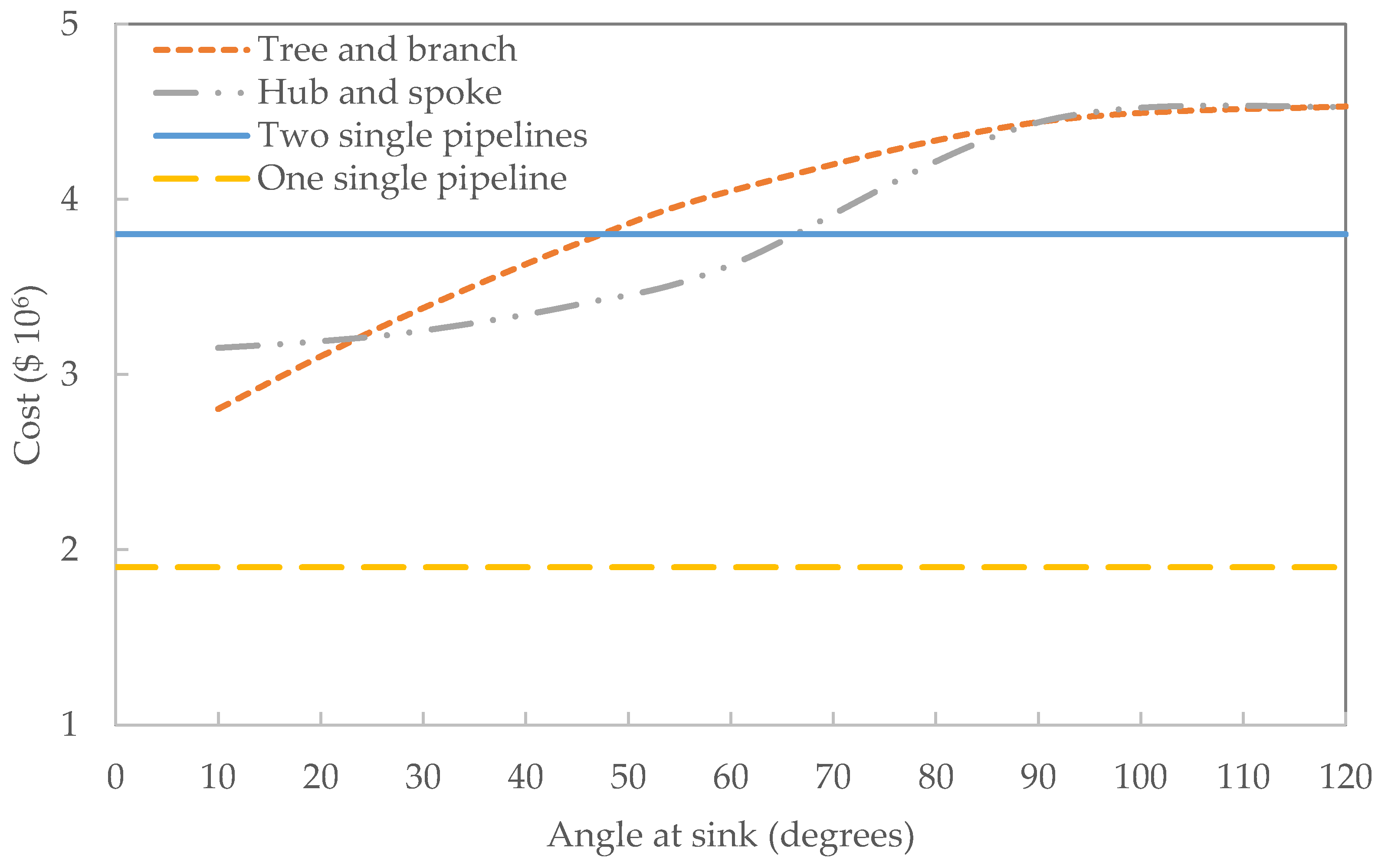
Both the inlet temperature and the surrounding temperature have an effect on the pressure drop and the distance where recompression is required. Lower input and ambient temperatures result in lower pressure losses and are more favourable to CO₂ pipeline transportation [37]. Figure 3 shows inlet temperature effect on the point of no-flow (or choking point) and safe distance of fluid flow before recompression. The safe distance is taken as 90% of the choking point. The plots from data obtained from Witkowski et al. [37] and Zhang et al. [63] are unrelated. Since temperature varies along a pipeline and has effects on the properties of CO₂ stream, it is necessary to take the temperature variations of the CO₂ stream into consideration while designing a pipeline. However, not many models consider this factor.

7. Pipeline Wall Thickness

Pipelines must have enough wall thickness to withstand the flowing and surrounding pressures. Pipes with inadequate thickness and strength can burst when exposed to high internal pressures or collapse when exposed to high external pressures. The maximum operating pressure dictates the pipe strength vis-à-vis the pipe wall thickness. Pipes having a higher wall thickness will withstand higher pressures without failing. Liquid CO₂ requires thinner pipes compared to supercritical CO₂ when transported under the same conditions in a pipeline [64]. Pipelines with wall thickness of 11.9 mm or more are resistant to damage and failure rate is low with reduced individual risk levels around these pipelines [65]. The expected burst and collapse pressures must therefore be calculated and used to select pipes with adequate wall thickness and strength. However, pipes with thicker walls are more expensive than thinner walled pipes. Pipe wall thickness is half the difference between the outer and inner diameters of a circular pipe. Witkowski et al. [37], and McCoy and Rubin [62] presented Equation (10) to calculate the pipeline wall thickness:

$$t=\frac{P_{max} D_o}{2 S E F}$$

(10)

where t = pipeline thickness (m), D_o = outer diameter of pipeline (m) P_max = maximum operating pressure (MPa), S = specific yield stress of pipe material (MPa), E = longitudinal joint factor (1.0) and F = design factor (0.72).

The thickness equation presented by Chandel et al. [27] and Lazic et al. [21] was slightly different. They used the internal diameter instead of the outer diameter and subtracted P_max from the product of S, E and F before multiplying by 2. Equations (10) and (11) both give exactly the same pipe wall thickness:

$$t=\frac{P_{max} D}{2\left(S·F·E-P_{max}\right)}$$

(11)

where D = internal diameter of pipeline (m).

The Knoope et al. [54] equation introduced a corrosion factor, CA. This factor increases the calculated value of the wall thickness by the assumed value of CA, see Equation (12):

$$t=\frac{D_o+ P_{max}}{2·S·F·E}+CA$$

(12)

where CA = corrosion allowance (0.001 m).

The equation presented in Kang et al. [66] includes location factor, L_f and temperature factor, T. Equation (13) gives pipe thickness values between those obtained with Equations (11) and (12):

$$t=\frac{P_{max} D_o}{2S F L_f E T}$$

(13)

where, F = 0.8, L_f = 0.9 and T = 1.0.

The fluid flow rate determines the pipeline internal diameter to transport the volume. The choice of the design parameters would affect the values calculated for the pipeline wall thickness. Pipes are designated with external diameter values or nominal pipe size (NPS). Two pipes can have the same NPS but different internal diameters if the pipe wall thickness is different. A pipe with a thicker wall will have a smaller internal diameter and more expensive than a pipe with a thinner wall.

8. CO₂ Stream Composition

CO₂ streams are usually not pure and may contain several impurities. The impurities in the stream affect the physical and thermodynamic properties of the flowing fluid. CO₂ stream composition depends on the source of CO₂, naturally occurring or captured from industrial processes. Percentages of impurities in captured CO₂ fluids vary according to the type of capture (pre-combustion, oxy-fuel or post-combustion); see

Table 3. CO₂ stream composition for different capture methods (volume%) [34,68].

Component	Post Combustion	Pre-Combustion	Oxy-fuel
CO2	>99	>95.6	>85
CH4	<0.01	<0.035	--
N2	<0.17	<0.6	<7
H2S	Trace	<3.4	trace
C2+	<0.01	<0.01	--
CO	<0.001	<0.4	0.075
O2	<0.01	Trace	<3
NOx	<0.005	--	<0.25
SOx	<0.001	0.07	<2.5
H2	Trace	<3	Trace
Ar	Trace	<0.05	<5
H2O	0.01	0.06	0.01

.

Table 4. CO₂ stream composition in mol % of some existing pipelines [35,59].

	Cortez Pipeline	Canyon Reef Carriers	Sheep Mountain	Central Basin Pipeline	Bravo Dome	Weyburn	Jackson Dome
CO2	95	85–98	96.8–97.4	98.5	99.7	96	98.7–99.4
CH4	1–5	2–15	1.7	0.2		0.7	Trace
N2	4	<0.5	0.6–0.9	1.3	0.3	<0.03	Trace
H2S	0.002	<0.02		<0.002 wt		0.9	Trace
C2+	Trace		0.3–0.6			2.3
CO						0.1
O2				<0.001 wt		<0.005 wt
H2						Trace
H2O	0.0257 wt	0.005 wt	0.0129 wt	0.0257 wt		0.002 v

shows compositions of some existing CO₂ pipelines for EOR. The Jackson Dome and Bravo Dome pipelines have the purest CO₂ streams with greater than 98.5% CO₂ while the Canyon Reef pipeline has the highest percentage of impurities with as low as 85% CO₂ concentration. The given range of concentration of fluid composition in Table 4 is an indication that the composition of some CO₂ streams may change. To design an effective CO₂ pipeline, a good knowledge of fluid phase, pressure, temperature, composition and mass flow rate is required [57,67].

When two or more streams mix during pipeline transportation of CO₂, the fluid composition after mixing has a major impact on phase behaviour and must be known. Brown et al. [57] looked at four different CO₂ capture scenarios for two pipelines that merged into one along the transport route and stated that it is essential to accurately model the pressure drop, fluid phase and stream composition. It is necessary to model continually the amount and composition of CO₂ streams produced even from the same source because it can change over time [57]. Since the density, phase behaviour and viscosity of rich CO₂ fluids are required to accurately model CO₂ pipelines [37,62], the actual composition of CO₂ streams must be known. Depending on the capture process and the purity of the feed fuel, the concentration and range of the impurities can be very large, see

Table 5. Minimum and maximum mole percentages of typical impurities in CO₂ streams [7,69,70,71,72].

	CO2	N2	O2	Ar	SO2	H2S	NOx	CO	H2	CH4	H2O	NH3
Min.%	75	0.02	0.04	0.005	<10−3	0.01	<0.002	<10−3	0.06	0.7	0.005	<10−3
Max.%	99.95	10	5	3.5	1.5	1.5	0.3	0.2	4	4	6.5	3

.

Most models assumed pure CO₂ streams but no CO₂ stream is 100% pure and therefore they are not quite accurate. All common impurities created a two phase region in a phase envelope and raised the critical pressure above 7.37 MPa [61] The effect of impurities on the properties of CO₂ is profound and modelling to represent practical situations is necessary.

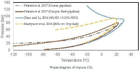
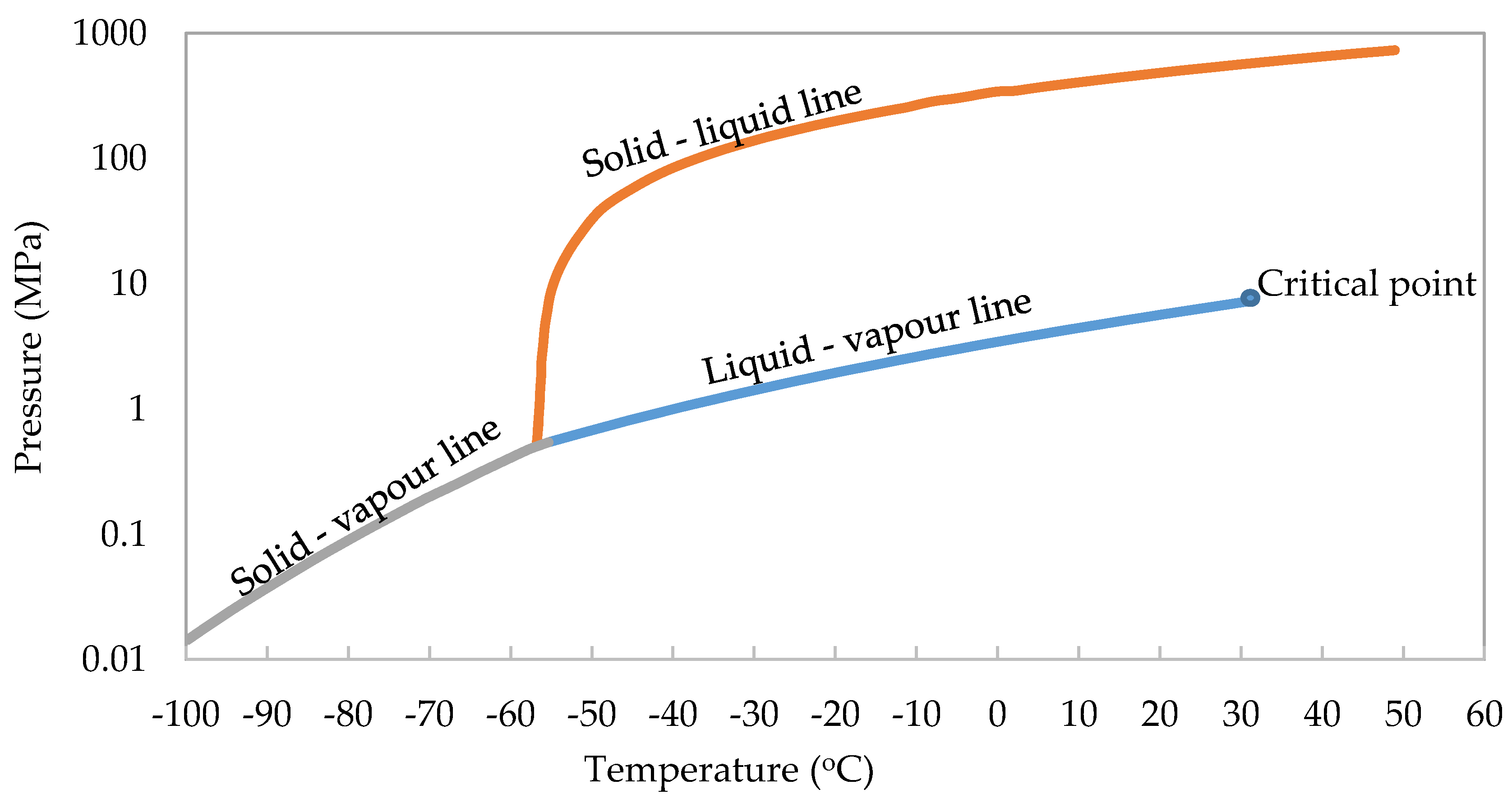
9. CO₂ Phases in Pipeline Transportation

CO₂ flows in pipelines as a gas, supercritical fluid and subcooled liquid [63]. Transporting CO₂ in any particular state has its advantages and disadvantages. All three states (gas, supercritical and liquid) of CO₂ exhibit different thermodynamic behaviour and the determination of the properties of the fluid is necessary for an effective design of CO₂ pipelines. Veritas [67] considered the Peng-Robinson equation of state (EOS) adequate for predicting mass density of CO₂ in gaseous, liquid and supercritical states but stated that there was need to verify the EOS for CO₂ mixtures with impurities, especially around the critical point. 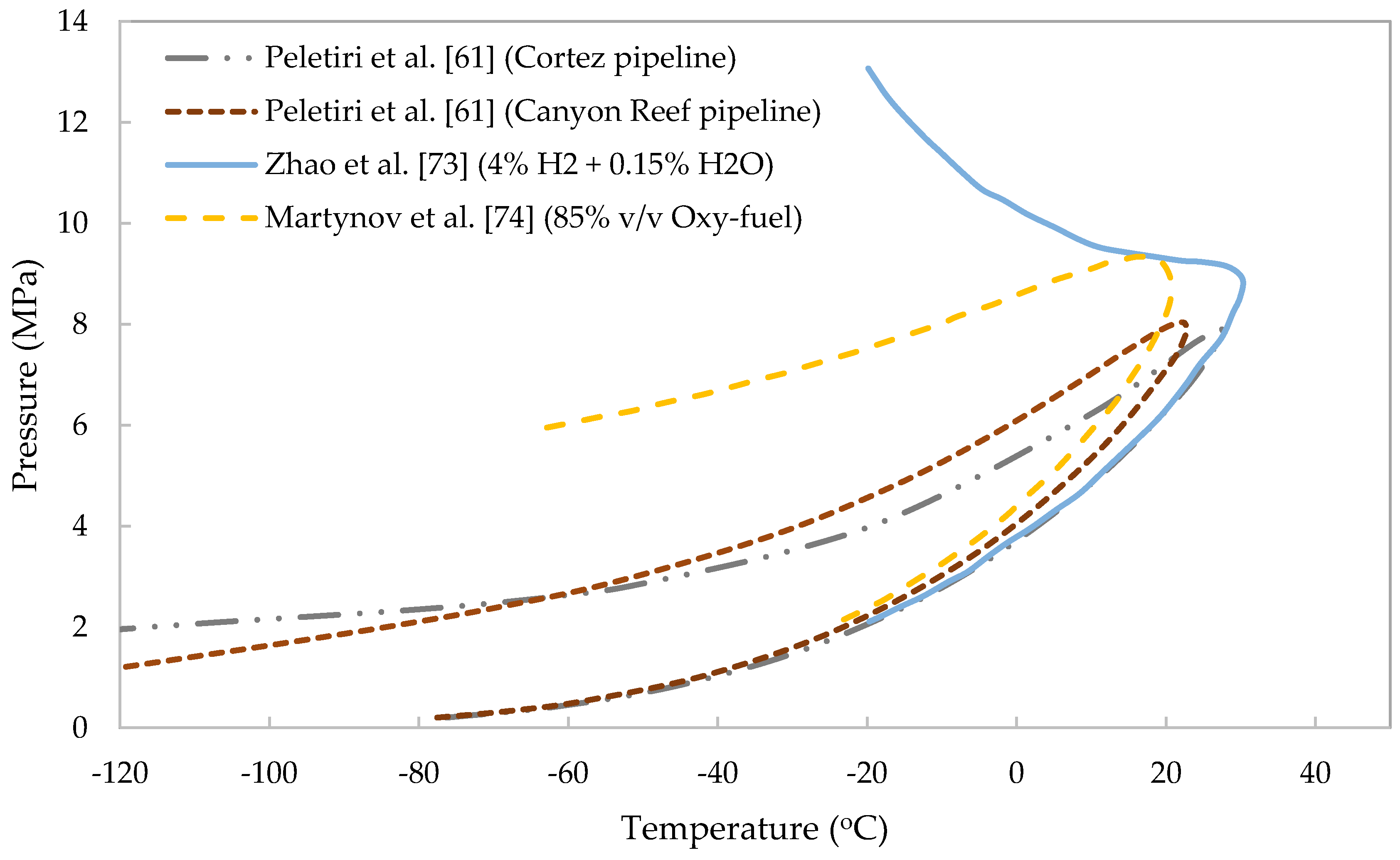The phase diagram of pure CO₂ shown in Figure 4 is different from that of CO₂ with impurities, shown in Figure 5. Different percentages of impurities result to different critical points and shapes of the phase diagram. Impurities create two-phase region where vapour and liquid coexist and pipelines are designed to operate outside this region to avoid flow assurance problems.

Generally, transporting gaseous CO₂ in pipelines is not economical due to the high volume of the gas, low density and high-pressure losses [62]. It may however, still be more cost effective to transport CO₂ in the gaseous state than in the liquid or supercritical states under certain circumstances. The Knoope et al. [75] model is capable of evaluating the more cost effective method between gaseous and liquid CO₂ transport. They stated that at CO₂ mass flow rate of up to 16.5 Mt/y with a distance of 100 km over agricultural terrain and 15.5 Mt/y with a distance of 100 km for offshore pipeline, transporting CO₂ in the gaseous state was more cost effective than in the liquid state. One advantage of transporting gaseous CO₂ in pipelines is the use of pipes with lower thickness (1% of outer diameter) resulting to lower material cost for pipelines [75].

Transporting CO₂ as a subcooled liquid and supercritical fluid is however preferred over gaseous CO₂ [41,76]. Subcooled CO₂ transport has some advantages over supercritical phase transport due to higher densities, lower compressibility and lower pressure losses. Some advantages of subcooled liquid CO₂ transportation over supercritical transportation according to Zhang et al. [63] include, use of smaller pipe diameter, transport of more volume due to the higher density and lower pressure losses. Teh et al. [64] concluded that transporting CO₂ in the subcooled liquid state is better than transporting it in the supercritical phase because thinner and smaller diameter pipes are adequate to transport liquid CO₂ but not supercritical CO₂ and that pumps consume less energy than compressors, resulting in 50% less energy requirement for liquid transport than for supercritical transport. Transporting CO₂ in liquid phase at low temperature (−40 °C to −20 °C) and 6.5 MPa results in lower compressibility and higher density than CO₂ in supercritical state [60]. This means that lower pressure losses occur and smaller pipe diameters are adequate for liquid CO₂ transportation with the requirement for fewer booster stations and thinner pipes thereby reducing capital cost. Subcooled liquid CO₂ transportation is however employed mainly in ship transportation at densities of about 1162 kg/m³ at 0.65 MPa and −52 °C [40]. One disadvantage of liquid CO₂ in comparison to supercritical CO₂ is the need to insulate pipelines in warmer climates.

CO₂ liquid pipeline transportation has some advantages over supercritical transportation, yet transportation in the supercritical phase has become a standard practice. The Office of Pipeline Safety in the US Department of Transportation defined pipeline CO₂ as a compressed fluid in supercritical state consisting of more than 90% CO₂ molecules [36]. Pipeline CO₂ fluid is mostly modelled as a single phase supercritical fluid.

10. Pipeline Diameter and Pressure Drop

Pipeline diameter and pressure drop are used to optimise the design of CO₂ pipelines. Available pipes with very large diameter could have been chosen but for the high costs. An optimum pipeline diameter is the smallest pipe diameter that is large enough for the volume of fluid transported without resulting to excessive velocities. An adequate pipeline diameter avoids excessive pressure losses and reduce number of boosting stations to optimise the cost of CO₂ transportation. An initial diameter is chosen with knowledge of fluid volumes and pressure losses, pressure boosting requirements and costs determined. It may be necessary to repeat this process with different diameter sizes before selecting an optimum pipeline diameter. More than one pipeline may be required if the largest available pipeline diameter is smaller than the calculated (optimised) diameter. Vandeginste and Piessens [39] stated that flow rate, pressure drop, density, viscosity, pipe roughness, topographic differences, and bends, all affect the determination of pipe diameter. Some researchers have proposed equations to calculate pipeline diameter and pipeline pressure drop. Below is a chronological presentation of some publications.

The IEA GHG [23] report gave equations for liquid pressure drop (Equation (14)), a form of Darcy′s formula and an equation for gas flow rate (Equation (15)), used for sizing of pipelines. Design criteria of outlet pressure greater than 0.6 MPa for liquid lines and a maximum velocity less than 20 m/s for gas pipelines were used. A velocity of 5 m/s for liquids and 15 m/s for gases used in equations to select initial diameter for the pipeline and pressure drop calculated and compared to the design criteria. If the criteria are met, the pipeline size is accepted otherwise, the diameter is increased to the next available normal pipeline size. The initial guess formed the basis for the pipeline sizing routine and there was no method to optimize the initial guess, which may result to oversizing of the pipeline. The pressure drop is usually specified from the maximum and minimum allowable pressures in CO₂ pipeline design. Equation (14) is used to calculate the distance of pipeline at which the pressure drops to the minimum value. This equation considered flow rate, length of pipeline, fluid density and pipeline diameter in the determination of pipeline pressure drop. The equation for gas flow has gas specific gravity in place of fluid density:

$$\Delta P=2.252 \frac{f L \rho Q_v^2}{D^5}$$

(14)

where ΔP = pressure drop (MPa), Q_v = flow rate (m³/s), f = friction factor, $\rho$ = density (kg/m³), and L = length of pipeline (m).

$$Q_v=15485\sqrt{\left[\frac{P_1^2-P_2^2}{f L SG}\right]D^5}$$

(15)

where Q_v = Gas flow rate (m³/s) and SG = specific gravity of gas relative to air.

Ogden et al. [77] presented a formula for supercritical flow rate as a function of pipeline inlet and outlet pressures, diameter of pipeline, average fluid temperature, length of pipeline, specific gravity, gas deviation factor and gas composition (Equation (16)). The calculated diameter depends also on the pipeline length and increases with increasing length. The fluid velocity therefore changes with different values of pipeline length even though the flow rate remains the same. This equation is not suitable for specifying optimum diameter size but can be rearranged to compute pipeline distances for the installation of boosting stations:

$$D^{-2.5}=\frac{1}{Q_v}{C}_1 \sqrt{\raisebox{1ex}{$1$}\!\left/ \!\raisebox{-1ex}{$f$}\right.} E {\left[\frac{\left(P_1-P_2-C_2 \left\{G \Delta h\frac{P_{ave}^2}{Z_{ave} T_{ave}}\right\}\right)}{G T_{ave} Z_{ave} L}\right]}^{0.5}$$

(16)

where Q_v = gas flow rate (Nm³/s), C₁, C₂ = 18.921 and 0.06836 (constants), E = pipeline efficiency, G = specific gravity of gas (1.519), T_ave = average temperature along the pipeline (°K) and Z_ave = average gas deviation factor.

As CO₂ travels along the pipeline, pressure drops and the fluid expands resulting to increased velocity, which further increases the pressure loss with the possibility of two-phase flow. Zhang et al. [63] specified safe distances to prevent two-phase flow or choking point at 10% less than the calculated choking distance. Boosting stations for recompression are installed at these safe distances. Adiabatic flow results to longer CO₂ transport distances than isothermal flow before recompression and subcooled flow covers 46% more distance than supercritical flow before boosting is required [63]. Pipeline distance, terrain, maximum elevation and insulation were some of the factors, included in their report for design considerations in long distance pipelines. Equation (17), the optimized hydraulic diameter equation, is a cost optimization equation. This equation is independent of pipeline length and may be suitable for specifying adequate pipeline diameter for specific fluid volumes:

$$D_{opt}=0.363 Q_v^{0.45} {\rho }^{0.13} {\mu }^{0.025}$$

(17)

where D_opt = optimum inner diameter (m), µ = gas viscosity (Pa·s).

Zhang et al. [63] used ASPEN PLUS (v1.01) to simulate the pipeline transportation of CO₂. Pressure drop calculations were made to specify maximum pipeline distances to prevent phase changes and pressure booster stations designed to be installed at 10% less than the distance of the computed value for potential phase change i.e., choking point.

Vandeginste and Piessens [39] derived Equation (18) after assuming that the velocity does not change along the pipeline and neglecting local losses. The velocity however, changes whenever there is a pressure change as the fluid expands or contracts. This assumption reduces the accuracy of their equation for the calculation of pipeline diameter. Equation (19) considers local losses with four solutions. The positive value that is higher than the value obtained without considering local losses (i.e., using Equation (18)) is the correct value:

$$D={\left(\frac{4^{10/3} \times n^2\times Q \times L}{{\pi }^2 {\rho }^2 \left(\left(z_1-z_2\right) + \left(\left(P_1-P_2\right)/\rho g\right)\right)}\right)}^{\raisebox{1ex}{$3$}\!\left/ \!\raisebox{-1ex}{$16$}\right.}$$

(18)

$$D={\left(\frac{1}{2}\sqrt{t_1+t_2}+\frac{1}{2}\sqrt{-t_1-t_2-\frac{2b}{\sqrt{t_1+t_2}}}\right)}^{3/4}$$

(19)

where:

$$t_1=\frac{\sqrt[3]{2/3a}}{\sqrt[3]{9b^2+\sqrt{81b^4-768a^3}}}$$

$$t_2=\frac{\sqrt[3]{9b^2+\sqrt{81b^4-768a^3}}}{3^{2/3 }\sqrt[3]{2}}$$

$$a=\frac{4^{10/3 }{n}^2 L Q^2}{{\pi }^2\left(z_1-z_2+\left(\left(P_1-P_2\right)/\rho g\right)\right)}$$

$$b=\frac{8 Q_m^2{{\displaystyle \sum }}_i{\xi }_i}{g{\pi }^2\left(z_1-z_2+\left(\left(P_1-P_2\right)/\rho g\right)\right)}$$

The Vandeginste and Piessens [39] model included the effects of bends along the pipeline, though the effect was found to be minimal. The model considered flow rate, pressure changes, fluid density, gravitational effect and elevation. They presented the Darcy–Weisbach formula for diameter calculation after incorporating the elevation difference (Equation (20)). This diameter equation, the hydraulic equation, is also a function of the length of pipeline. Computing diameter values with varying pipeline length would result in varying diameter values for the same volume of fluid flowing in the pipeline:

$$D={\left[\frac{8 f Q^2 L}{\rho {\pi }^2 \left[\rho g \left(z_1-z_2\right) + \left(P_1-P_2\right)\right]}\right]}^{\frac{1}{5}}$$

(20)

The diameter of some pipelines were calculated and compared to the values to the actual diameters of the pipelines [39]. Their results show that the computed diameter values were consistently smaller than the actual diameters of the pipelines. One reason for this is that actual pipeline diameters are available nominal pipe sizes (NPS) with internal diameter equal to or greater than the computed values.

McCoy and Rubin [62] calculated pipeline diameter by holding upstream and downstream pressures constant. With the assumption that kinetic energy changes are negligible (constant velocity) and compressibility averaged over the pipeline length, the pipeline internal diameter, Equation (21), as derived by Mohitpour et al. [78] is:

$$D={\left\{\frac{-64 Z_{ave}^2 R^2{T}_{ave}^2 f_F Q^2 L}{{\pi }^2\left[M Z_{ave} R T_{ave}\left(P_2^2-P_1^2\right) + 2 g P_{ave}^2 M^2\left(z_2-z_1\right)\right]}\right\}}^{\raisebox{1ex}{$1$}\!\left/ \!\raisebox{-1ex}{$5$}\right.}$$

(21)

where T_ave = average fluid temperature (K), M = molecular weight of flowing stream.

Since the fanning friction factor depends on pipe diameter, Equation (22) by Zigrang and Sylvester was used to approximate f_F:

$$\frac{1}{2\sqrt{f_F}}=-2.0 lo{g}_{10}\left\{\frac{\epsilon /D}{3.7}-\frac{5.02}{R_e}log\left[\frac{\epsilon /D}{3.7}-\frac{5.02}{R_e}log\left(\frac{ϵ/D}{3.7}+\frac{13}{R_e}\right)\right]\right\}$$

(22)

where ε = pipe roughness factor (m), f_F = fanning friction factor

This model considered temperature, pressure drop, pipeline friction factor, elevation change, fluid compressibility, molecular weight, flow rate with an assumed constant temperature at an average value equal to ground temperature. The assumption of constant velocity and constant temperature reduces the accuracy.

Chandel et al. [27] based the determination of CO₂ pipeline diameter on inlet and outlet pressures and length of pipeline. Pipelines were assumed to be buried 1 m below the surface with a constant density and constant temperature of 27 °C. The input pressure of all CO₂ sources was kept constant at 13 MPa and CO₂ flow rate and velocity were the only variable inputs into diameter estimation equation. A fixed density of CO₂ (827 kg/m³) was used, assuming temperature was at a constant 27 °C with a constant average pressure of 11.5 MPa. Equation (2) was used to calculate the pipe inner diameter and the pipeline wall thickness with Equation (11). Where the calculated diameter is larger than the largest available standard diameter, a single pipeline would not be sufficient to transport the flow rate and Equation (23) is used to calculate the minimum number of pipelines needed.

$$N_{pipe}=\lfloor \frac{Q_v}{Q_{ v,max}}\rfloor +1$$

(23)

where N_pipe = number of pipes, $\lfloor \frac{Q_v}{Q_{v,max}}\rfloor$ = the integer value of $\frac{Q}{Q_{max}}$ less than or equal to the enclosed ratio (magnitude), and Q_v,max = maximum flow rate in the pipe with the largest diameter (m³/s). Where more than one pipeline is required, there is need for an economic analysis to optimise the sizes of the pipelines. If $N_{pipe}-1$ pipes have diameter ${D_i}_{max},$ then $N_{pipe}^{th}$ pipe diameter is calculated using Equation (24):

$$D_o{}_{N_{pipe}^{th}}=\sqrt{\frac{4 \left[Q-\left(N-1\right)Q_{v,max}\right]}{\pi V}}$$

(24)

where $D_{o N_{pipe}^{th}}$ = outer diameter of the nth pipe (m).

Pressure drop is calculated with Bernoulli′s equation (Equation (25)) with the inherent assumption of constant velocity, which neglects acceleration losses:

$$P_1-P_2={10}^{-6} \rho g \left(h_L+\Delta z\right)$$

(25)

where ρ = density of supercritical CO₂ (827 kg/m³), h_L = head loss (m), and z = gas deviation factor.

Friction is the dominant cause of head loss and is calculated using Equation (26), the Darcy-Weisbach equation:

$$h_f=f\times \frac{l v^2}{2 D g}$$

(26)

where h_f = frictional head loss (m), l = length between booster stations. Where the pipeline is transporting less than full capacity, the actual velocity of fluid flow is calculated with Equation (2). This is applicable in oversized pipelines before the second stream comes online. Rearranging after combining Equations (25) and (26) and neglecting a change in elevation gave Equation (27), the equation for calculating length of pipeline that would require a booster station assuming a horizontal pipeline. Equation (27) is the same as Equation (20):

$$l=\frac{\Delta P}{\rho f}\times \frac{2 D_i}{v^2}$$

(27)

Friction factor which depends on the pipe roughness, internal diameter and flow turbulence is calculated with Equation (28), the Haaland equation:

$$\frac{1}{\sqrt{f}}=-1.8 {\log }_{10}\left[{\left(\frac{\epsilon /D_i}{3.7}\right)}^{1.11}+\frac{6.9}{Re}\right]$$

(28)

where ε = roughness factor, (4.5 × 10⁻⁵ m for new pipes but 1.0 × 10⁻⁵ m was assumed).

They showed that the number of booster pump stations is equal to the total pipeline length L divided by the distance of pump stations l_i using Equation (29):

$$N_{pump}=\frac{L}{l_i}$$

(29)

where $N_{pump}$ = number of pump stations, and l_i = number of pipeline sections.

At the end of the pipeline, an additional pump station is used to raise pressures to 13 MPa for delivery. The equation for electric power required to increase the fluid pressure back to 13 MPa is Equation (30) [79]:

$$W_{pump}=\frac{Q\left|P_{l_i-}{P}_{initial}\right|}{{\eta }_p}$$

(30)

where ${\eta }_p$ = pump efficiency assumed to be 0.75, and W_pump = pump power requirement (W).

The Chandel et al. [27] model presented separate equations to calculate pipeline pressure drop and/or pipeline diameter, pipeline thickness, number of pipelines required to transport any particular CO₂ flow rate, velocity of fluid flow, number of booster stations required and frictional head losses. However, constant temperature, density, compressibility and average pressure was assumed. These many assumptions affect the accuracy of the model. The assumption of constant soil temperature is not practical because there is heat exchange between the pipeline and the surrounding (soil). The temperature either increases in warm climate or decreases in cold climate along the direction of flow even with insulated pipelines. There may also be seasonal changes of surrounding temperatures between low temperatures in winter and high temperatures in summer. The input pressure of 13 MPa for all CO₂ inlets may cause a “no-flow” because pressure difference (ΔP) between any two CO₂ input points along the pipeline would be zero. The CO₂ stream pressure at any additional input point should be calculated and input pressures specified accordingly. Alternatively, a booster station may be installed just before input points to raise the pressure to 13 MPa equal to that of the incoming stream.

IEA GHG [55] report recasting the velocity equation (Equation (2)) as Equation (31) by moving the constant 4 to the denominator as 0.25 and making the diameter the subject of the formula:

$$D={\left(\frac{Q_m}{v\times \pi \times 0.25\times \rho }\right)}^{0.5}$$

(31)

Pressure drop per length ($\raisebox{1ex}{$\Delta P$}\!\left/ \!\raisebox{-1ex}{$L$}\right.$) is calculated in three steps. First, the Reynolds number is calculated, then the friction factor and finally the pressure drop per unit length (Equations (32)–(34)). Equation (34) is the same as Equation (20) but without the elevation component of pressure drop. The maximum pipeline length, l_max between two booster stations is given by Equation (35). This report considered only pressure losses due to friction:

$$Re=\raisebox{1ex}{$\rho v D$}\!\left/ \!\raisebox{-1ex}{$\mu $}\right.$$

(32)

$$f=\raisebox{1ex}{$1.325$}\!\left/ \!\raisebox{-1ex}{${\left[ln\left(\left(\epsilon /3.7D\right)+\left(5.74/R{e}^{0.9}\right)\right)\right]}^2$}\right.$$

(33)

$$\raisebox{1ex}{$\Delta P$}\!\left/ \!\raisebox{-1ex}{$L$}\right.=\frac{8 f Q^2}{\rho {\pi }^2{D}^5}$$

(34)

$$l_{max}= \frac{P_1 - P_2}{\Delta P/L}$$

(35)

Knoope et al. [75] analysed both gaseous and liquid CO₂ pipeline transportation with inlet pressures of 16 to 3 MPa for gaseous transport and 90 to 24 MPa for liquid transport. A high erosional velocity of 6 m/s was set for liquid lines with a minimum velocity of 0.5 m/s to ensure flow. Equation (36), a cost optimisation equation, is used to calculate the specific pressure drop, which is then used to calculate the diameter of the pipeline. Calculating the pressure drop before the diameter would require equations that are functions of pipeline length:

$$\Delta P_{design}=\frac{\left(P_1-P_2\right)\times \left({\eta }_{booster}+1\right)}{L}+\frac{g\times \rho \times \Delta z}{L}$$

(36)

Knoope et al. [48] presented five diameter equations; velocity based (Equation (2)), hydraulic (Equation (34)), extensive hydraulic model (Equation (18)), the McCoy and Rubin [62] (Equation (21)) and Ogden et al. [77] model (Equation (37)). They computed pressure drop for a specified pipeline length before calculating pipeline diameter. Elevation, inlet and outlet pressures, number of booster stations and length of the pipeline were considered in the determination of pipeline diameter:

$$D={\left\{\frac{G\times Z_{ave} \times T_{ave}\times Q^2 \times f \times L\times {\eta }_{pipe}^2}{a_1 \left[{\left(\frac{P_1}{1000}\right)}^2-{\left(\frac{P_2}{1000}\right)}^2-\left(a_2 \times G \times \frac{P_{ave}}{1000} \times Z_{ave}\times T_{ave}\times \Delta h\right)\right]}\right\}}^{\raisebox{1ex}{$1$}\!\left/ \!\raisebox{-1ex}{$5$}\right.}$$

(37)

where R = Gas constant (8.31 Pa·m³/mol K), G = specific gravity (1.519), η_pipe = efficiency of pipeline (assumed = 1.0), a₁ and a₂ = constants equal to 73.06 and 0.006836 respectively.

Lazic et al. [21] separated the diameter equations into turbulent flow- (Equation (34)) and velocity-based (Equation (2)). The equations for cost optimization (Equation (17)) and liquid pressure drop (Equation (27)) were also given. They stated that pressure drop for both liquid and dense phases can be calculated with Equation (34).

Kang et al. [66] added pressure changes due to changes in elevation into Equation (34) to derive Equation (38), which is the same as Equation (20):

$$\Delta P=\frac{8 f Q_m^2 L}{\rho {\pi }^2 D^5}+\rho g \Delta Z$$

(38)

In an earlier publication, Kang et al. [17] gave an analysis of pipeline diameter, number of booster stations and total cost of CO₂ pipeline. They made 2-inch increments of NPS from 6 inches to 20 inches and found out that the smallest diameter gave an unreasonable high number of booster stations thereby increasing the cost of the project. The 14-inch pipe gave the minimum total cost of the pipeline. Figure 6 shows the pressure drop as a function of pipeline diameter. The lines in Figure 6 are plotted with different parameters but both lines show that a doubling of pipeline diameter reduced the pressure drop to about 4% of the initial value. To design booster installation along a pipeline, a minimum pressure is specified. The distance for the flowing fluid pressure to reduce to the minimum value is calculated and a booster station installed. The distances between booster stations may not be equally spaced along the same pipeline due to variations in elevation.

Brown et al. [57] reviewed four different CO₂ capture and transportation scenarios for two pipelines that merged into one along the transport route. The scenarios were post combustion capture for both pipelines, oxy-fuel for both pipelines and post combustion for one pipeline and oxy-fuel for the other. It was concluded that it is essential to accurately model the pressure profile, changes in fluid phases and composition of the fluid stream while designing CO₂ pipelines. Temperature and pressure may change along the pipeline as a result of frictional pressure losses, expansion work done by the flowing fluid and heat exchange between fluid and the surrounding. The Darcy friction factor (for turbulent flow) was calculated from Equation (33). The overall heat transfer coefficient is given in Equation (39):

$$\alpha ={\left[\frac{1}{{\alpha }_f}+\frac{D}{2{\lambda }_w}ln\left(\frac{D_o}{D}\right)+\frac{D}{2{\lambda }_{ins}}ln\left(\frac{D_o+{\delta }_{ins}}{D}\right)+\frac{D}{2{\lambda }_{soil}}ln\left(\frac{d_{soil}}{D}\right)+\frac{1}{{\alpha }_{amb}}\frac{D}{2d_{soil}}\right]}^{-1}$$

(39)

where $\alpha$ = overall heat transfer coefficient (W·m⁻²·K⁻¹), ${\lambda }_w$ = thermal conductivity of pipe wall (W·m⁻¹·K⁻¹), ${\lambda }_{ins}$ = thermal conductivity of insulation (W·m⁻¹·K⁻¹), ${\lambda }_{soil}$ = thermal conductivity of surrounding soil (W·m⁻¹·K⁻¹), ${\alpha }_f$ = heat transfer coefficient of internal pipe wall (W·m⁻²·K⁻¹) and ${\alpha }_o$heat transfer coefficient of external pipe wall (W·m⁻²·K⁻¹). The Brown et al. [57] model accounted for the effect of friction, heat flux or heat transfer between fluid and surrounding, temperature and thermal conductivity of the soil.

Skaugen et al. [80] stated that soil thermal conductivity and ambient temperature affect the pressure drop of the pipeline and should be known for accurate modelling. A combination of higher soil conductivity and lower ambient temperatures reduce the temperature of the flowing fluid and result to lower specific energy consumptions. It was also stated that small pipeline diameters might not be sufficient to conduct the heat generated from compression out of the pipeline during transportation, bringing the fluid to a more gaseous state. However, the assumed minimum pressure of 9 MPa would keep the fluid in the supercritical state. The pressure loss equation (Equation (40)) is just Equation (34) presented with different parameters:

$$\frac{\Delta P}{\Delta L}=-f \frac{{\dot{\dot{M}}}^2}{2 \rho D}$$

(40)

where $\dot{\dot{M}}$ = mass flux (kg/m² s).

Tian et al. [50] modified Equation (17) by using density and viscosity values calculated at average pressure and temperature along the pipeline, (see Equation (41)). Diameter values calculated with this equation are too low so the equation is not considered any further:

$$D=0.363 Q^{0.45}{\left[\rho \left(P_{ave},T_{ave}\right)\right]}^{-0.32}{\left[\mu \left(P_{ave},T_{ave}\right)\right]}^{0.025}$$

(41)

11. Discussion

The diameter and pressure loss equations have essentially remained the same over the years without significant changes. The pipeline diameter equations can be group into two broad categories. The first category is independent of pipeline length (Equations (2) and (17)) and the second category depends on pipeline length (Equations (16), (18), (20) and (21)). Equations that are functions of pipeline length are not suitable for the determination of optimum pipeline diameter. This is because the diameter value increases with increasing length of pipeline. A pipeline diameter can be calculated with these equations only after specifying pipeline length or pipeline section and pressure drop. This diameter, however, would not be optimal. The optimum pipe diameter is a product of economic considerations for least cost (capital and operational costs) [81]. Pipeline diameter should be a function of flow rate, density and maximum velocity [39] but independent of pipeline length. Equations that are independent of pipeline length (Equations (2) and (17)) are suitable for the selection of the size of optimum pipeline diameter. A simulation in a general Purpose Programing Software (gPROMS) by varying the flow rate from 200 to 370 kg/s while holding every other parameter constant changed the resultant velocity by 0.61% with Equation (17) and 39.9% with Equation (2). Equation (17) is therefore seen to be more accurate and is recommended over Equation (2).

After specifying the optimum diameter, the distance at which the pressure drops to the predetermined minimum is computed with the equations that are functions of pipeline length for the installation of booster stations. It should be noted that the calculated optimum diameter is the minimum internal pipeline diameter, adequate for the volume of fluid transported. This value may not correspond to available NPS (internal diameter plus pipe wall thickness). The selected pipe size is the smallest NPS with an internal diameter that is larger than or equal to the calculated optimum value and this is the value used in further computations. The values obtained with Equations (14) and (21) are too low resulting to high flow velocities. The units of Equation (14) seem to be incorrect. Equation (27) (the same as Equations (14), (34), (38) and (41)) could be rearranged to calculate the diameter. The optimal diameter of a CO₂ pipeline is a diameter that gives the lowest overall cost of CO₂ pipeline transportation. Analysis of the net present value of the pipeline cost is a good indication of the optimum cost of a CO₂ pipeline [82]. It may be necessary to analyse several pipeline diameter sizes, starting with the calculated value to arrive at the optimum value for any particular pipeline. The optimum pipeline diameter could be defined as the diameter of a pipeline that gives the minimum overall cost discounted to present value.

A 200 km pipeline with inlet and outlet pressures of 15 and 10 MPa respectively (pressure drop of 5 MPa) was assumed and diameter values simulated in gPROMS.

Table 6. Diameter prediction for 200 km pipeline with model formulae and resultant fluid velocity.

Equation No.	Ref.	Formula for Diameter (Di)	Diam. (m)	Min. Fluid Velocity (m/s)
(2)	[27,50]	${\left(\frac{4 Q_v}{\pi v}\right)}^{0.5}$	0.372	3.93
(14)	[23]	${\left[2.252 \frac{f·L·\rho ·Q_v^2}{\Delta P}\right]}^{1/5}$	0.165	6.629
(16)	[77]	$\frac{1}{Q_v}{C}_1 \sqrt{\raisebox{1ex}{$1$}\!\left/ \!\raisebox{-1ex}{$f$}\right.} E {\left[\frac{\left(P_1-P_2-C_2 \left\{G \Delta h\frac{P_{ave}^2}{Z_{ave} T_{ave}}\right\}\right)}{G T_{ave} Z_{ave} L}\right]}^{0.5}$	0.742	0.987
(17)	[63]	$0.363 Q_v^{0.45} {\rho }^{0.13} {\mu }_c^{0.025}$	0.460	2.562
(18)	[39]	${\left[\frac{4^{10/3}{n}^2{Q}_m^2 L}{{\pi }^2{\rho }^2\left[\left(z_1-z_2\right)+\raisebox{1ex}{$\left(P_1-P_2\right)$}\!\left/ \!\raisebox{-1ex}{$\rho g$}\right.\right]}\right]}^{3/16}$	0.859	0.735
(20)	[39]	${\left[\frac{8 f Q_m^2 L}{\rho {\pi }^2\left[ \rho g \left(z_1-z_2\right)+\left(P_1-P_2\right)\right]}\right]}^{\frac{1}{5}}$	0.667	1.222
(21)	[62,78]	${\left\{\frac{-64 Z_{ave}^2 R^2{T}_{ave}^2 f_F Q^2 L}{{\pi }^2\left[M Z_{ave} R T_{ave}\left(P_2^2-P_1^2\right) + 2 g P_{ave}^2 M^2\left(z_2-z_1\right)\right]}\right\}}^{\raisebox{1ex}{$1$}\!\left/ \!\raisebox{-1ex}{$5$}\right.}$	0.256	8.250
(27)	[27]	$\frac{\rho f v^2 L}{2 \Delta P}$	0.667	1.222
(35)	[55]	${\left(\frac{8 f L Q_m^2}{\rho {\pi }^2\Delta P}\right)}^{1/5}$	0.667	1.222
(41)	[50]	$\frac{\Delta P}{\Delta L}=-f \frac{{\dot{\dot{M}}}^2}{2 \rho D_i}$	0.667	1.222

shows the diameter values obtained with the equations and the resulting velocity of the fluid stream. The velocity values shown in Table 6 are the minimum values calculated at the inlet of the pipeline. The fluid velocity increases along the direction of flow as the fluid expands due to reduced pressures.

Aspen HYSYS (a widely used commercially available software) simulation of pure CO₂ fluid with the same parameters used in gPROMS, using different thermodynamic equations of state gave diameter values of 0.554 m (SRK), 0.545 m (PR), 0.545 m (PR-TWU), 0.549 m (PRSV), and 0.554 m (SRK-TWU). Comparing these values to the diameter dependent equations shows that the hydraulic equation, Equation (20), performed better than the other equations with a minimum diameter difference of 0.117 m. This equation also gave a minimum resultant velocity value of 1.22 m/s and is seen as the most accurate.

12. Conclusions

Many aspects of CO₂ pipeline design have been reviewed with emphasis on available models for the determination of pipeline diameter in the literature. Two broad categories of equations for the determination of pipeline diameter were identified. Category one equations do not consider length of pipeline for the calculation of diameter while category two equations are dependent on pipeline length. Diameter equations that are functions of pipeline length should not be used for the initial specification of optimum pipeline diameter because the diameter value changes with varying pipeline length. Diameter equations that are independent of pipeline length should be used to select adequate pipeline diameter for the volume of fluid before using length dependent equations to specify pipeline distances for the installation of booster stations. The following were identified in this review.

• Impurities affect the density, pressure and temperature changes, critical pressure and temperature and viscosity but most models ignored the effects of impurities. Pressure loss values calculated with the assumption of pure CO₂ will therefore be inaccurate.
• No model considered pressure loss due to acceleration of the fluid, which is present whenever there is a change of velocity in the flowing fluid.
• The accurate determination of density and viscosity of the CO₂ fluid with impurities will improve the accuracy of the pipeline diameter and pressure drop models.
• Fluid velocity in the pipeline is calculated at the inlet is the minimum value in the pipeline. Maximum velocity occurs at the end of the pipeline section and should be incorporated into equations to avoid flow velocities above the erosional value.
• Diameter equations that are dependent of pipeline length are unsuitable for the estimation of optimum pipeline diameter. These equations estimate diameter sizes increasing with increasing pipeline length.

Further work is ongoing by the authors to model the effect of impurities and the contribution of losses due to acceleration in the pipeline for the specification of optimum diameter.