The Effect of a Wave Energy Farm Protecting an Aquaculture Installation

Abstract

This paper assesses the impact of a farm of wave energy converters on a nearby offshore aquaculture installation and on the nearshore dynamics. The coastal area targeted is Aguçadoura, located in the north of Portugal, where the world’s first wave farm operated in 2008. The study is focused mainly on the evaluation of the sheltering effect provided by the wave farm to the aquaculture cages. Furthermore, the possible impact on the coastal wave climate of such an energy park is also evaluated. These objectives are accomplished by performing simulations, corresponding to the wave conditions, which are more often encountered in that coastal environment. The SWAN model (Simulating WAves Nearshore) was adopted for this. Various transmission scenarios are considered to account for the impact of different types of wave converter farms on the downwave conditions. The results show that such a wave energy park might have a clear positive impact on the wave conditions fish farm installed downwave and it might also have a beneficial influence on shoreline dynamics from the perspective of coastal protection.

1. Introduction

Aquaculture and the energy extraction from the waves are two subjects in increasing development, becoming an interesting issue for the scientific community. A review of global research in fisheries science was done in [1]. Using statistics (1991–2013) from the Centre for Science and Technology Studies at the University of Leiden, the authors presented a significant increase in the number of publications in fisheries research (from 2000 in 1991 to 4750 in 2013). Regarding the energy that can be extracted from the ocean, a review about tidal and wave energy development in Europe, with current status and future perspectives, was presented in [2]. Wave energy is attracting more interest and investments than the tidal sector, with 45 companies at advance stages of development compared to 30 companies [2]. The authors in [2] demonstrated the barriers encountered for ocean energy progress. The worldwide increase of fish consumption requires alternatives to supply the seafood market and aquaculture has been responsible for this supply with a growth from 7% to 48.4% between 1974 and 2009 [3,4]. Herewith, employments emerge, but with differences between men and women. These differences were analyzed by [5], taking into account five points: the division of labor, the distribution of benefits, the access and control over assets and resources, social norms, and governance.

Regardless of the positive side of aquaculture as being an alternative to global fishery resources, it also might raise concerns related to issues such as: pollution, disease transmission, socio-economic impacts [6] and impacts on wild fish, namely in respect to disease propagation and, in the case of escapees from the farm, to food competition and interbreeding. One way to minimize these negative impacts is to move the aquaculture farms from coastal to offshore waters [6].

Offshore aquaculture can be defined, in the finfish farm community, as being the activities taking place in locations that are exposed to ocean waves [7], increasing the exposure to high wave energy due to the lack of shelters (such as islands and headlands), which can mitigate the force of both swell and locally generated waves [7]. A classification of the local wave climate, considering the values of the significant wave height (Hs), was introduced by the Norwegian government as described in [7]. The classification is defined by classes from 1–5, where class 1 is related to Hs < 0.5 m (the equipment has a small degree of exposure), class 2 is related to Hs of 0.5–1.0 m (the equipment has a moderate degree of exposure), class 3 is related to Hs of 1.0–2.0 m (the equipment has a medium degree of exposure), class 4 is related to Hs of 2.0–3.0 m (the equipment has a high degree of exposure) and class 5 is related to Hs > 3.0 m (the equipment has an extreme degree of exposure) [7]. This classification helps to choose the capabilities that the equipment needs to have, according to the site.

Some studies have focused in physical structures and on the sustainability of an aquaculture farm, as [8] with a design of a mooring system for a very large construction and [9] with a renewable energy solution for the automation power required for installations. Portugal is the most western country of the continental Europe, being surrounded on its western and southern sides by the North Atlantic Ocean. Due to its relatively large coastal area, its economy is strongly linked to water activities and according to [10] Portugal has the highest request per capita of seafood in Europe. Almeida et al. [11] suggested five main issues in order to give an explanation for the reason seafood is so appreciated in Portugal, and those are: geography (76% of people live in coastal areas), resources (high diversity in marine species), fisheries (cultural heritage and a way of subsistence), social forces, and politics.

Greenhouse gas emissions are one of the most recognized factors in anthropogenic climate changes. From this perspective, technological innovation in renewable energy is fundamental to achieving proposed emissions targets [12]. Earth’s seas and oceans have a high energy potential that can be extracted in various ways, marine energy being identified as a key element for a sustainable energy mix [13]. Besides offshore wind, it has been generally recognized that both wave and tidal energy resources exhibit significant potential for power generation, with some ambitious international targets for 2020 [14]. Moreover, according to many projections [15], by 2050 the electricity extracted from the ocean might be higher than today’s wind and solar electricity capacity, considered together. Nevertheless, if comparing them with the more traditional energy resources, they still must establish themselves commercially.

Over the last decade, various developers have been successful in demonstrating that it is possible to harvest energy from waves, and a wealth of device prototypes are now installed in European and International waters. In fact, the entire industry has now reached a turning point, where the current challenge is to develop the confidence required for large capital investment. At this critical time, besides improving the energy efficiency by developing more advanced power take-off systems, an important step towards commercial exploitation is represented by lowering the production cost by combining Wave Energy Converters (WECs) in arrays and optimizing in this way installation and maintenance costs, to make wave energy economically viable.

The wave energy resource can be assessed by wave models, such WAM (Wave model) [16], WW III (Wave Watch III) [17] and SWAN (Simulating WAves Nearshore) [18]. These are third-generation models that account for wave generation in the ocean offshore (WAM and WW III) and wave propagation in coastal areas (SWAN). The SWAN model has in consideration the physical processes that occur in shallow waters, such as bottom friction, depth-induced wave breaking, triad nonlinear interactions, refraction, and diffraction.

The use of wave models to evaluate wave energy potential was adopted in various studies. With an unstructured WW III version, the wave energy resource for Chile was evaluated between 2009 and 2010 [19]. The SWAN model was adopted to perform a coastal wave energy assessment in the Bohai sea [20] and western coast of Orkney [21]. Nested approaches among wave models (for wave generation and nearshore propagation) are often used, which is the case of [22], which used a wave prediction system with WAM and SWAN to assess the resource in Sweden. A review of the wave energy resource for different countries is presented in [23].

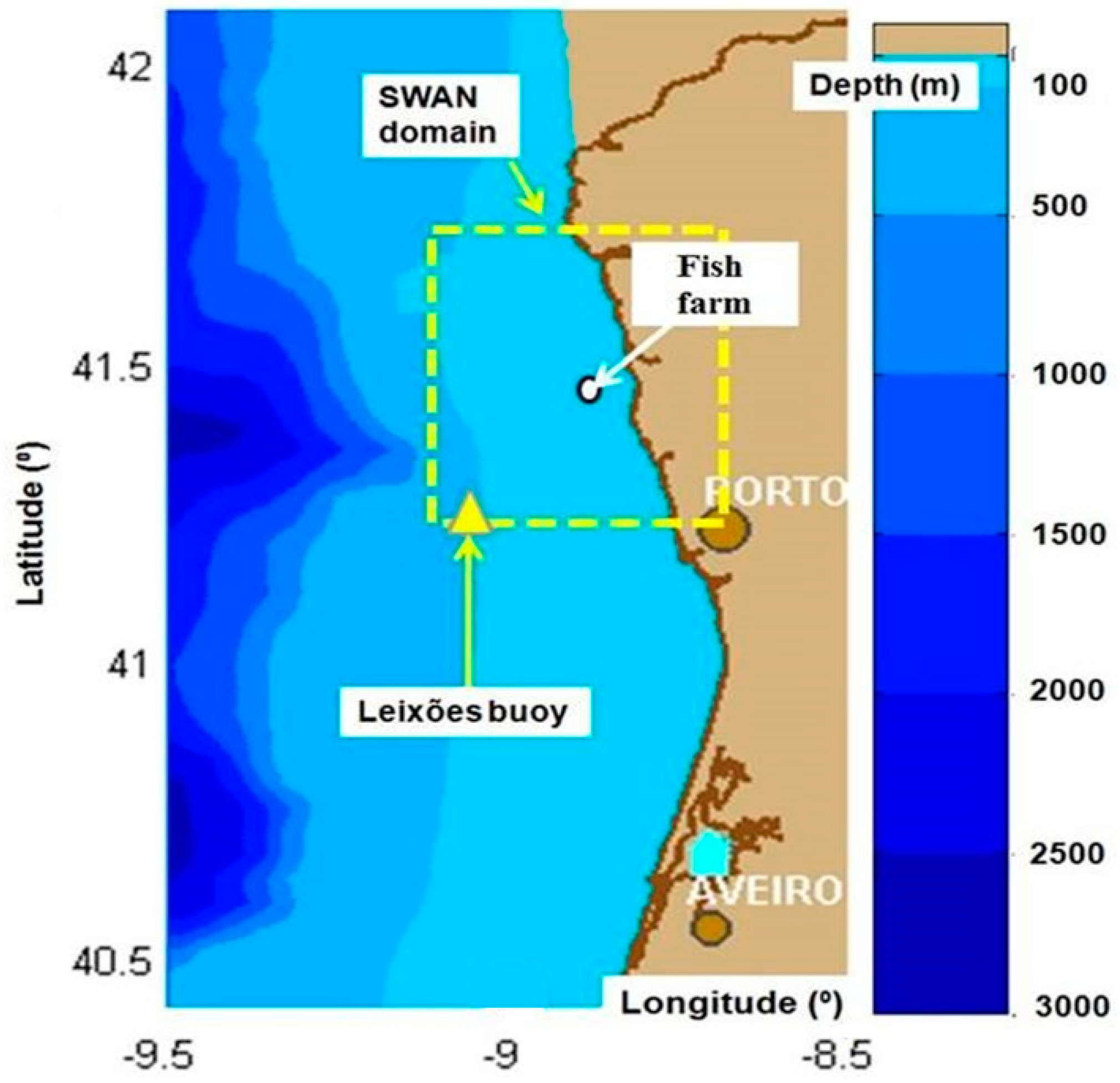
The Portuguese coastal environment, both continental [24] and the two archipelagos [25,26], has been identified with significant wave energy resources. From this perspective, Portugal has been a target for developments in this area. In fact, in 2008 the world’s first wave farm, composed of three Pelamis devices, was installed in Aguçadoura, north of Porto (the respective coastal environment is indicated with a yellow rectangle in Figure 1).

WECs, when capturing energy from waves, decrease the energy of the transmitted wave system and some studies have considered the impact on the beaches [27,28,29,30,31,32,33,34,35,36]. This decrease in wave energy makes a WEC farm a good option to protect marine structures without extra investments.

In this sense, the main goal of this paper is to estimate the possible impact of a wave farm, used as a sort of floating breakwater in providing sheltering and leading to an attenuation of waves, which reach a fish farm in the vicinity. Furthermore, the expected influence of the marine energy farm on the downwave nearshore wave climate up to shoreline level is also assessed.

2. Modelling the Wave Propagation in the Target Area

The evaluation of the effect of the marine energy farm on the downwave conditions up to the shoreline was done using simulations from the SWAN model. SWAN solves the action balance Equation (1). This is an advection-type Equation, which reflects the propagation of the action density spectrum in a space with five dimensions, defined by time, geographical and spectral spaces. At this point it must be highlighted that in SWAN the 2D spectral space considers the relative radian frequency and the wave direction.

$$\frac{\partial N}{\partial t}+\overline{V}gra{d}_{G-S}\left(N\right)=\frac{S}{\sigma }$$

(1)

The action density (N) is integrated in the SWAN governing Equation instead of the energy density spectrum (E), because unlike the energy density, the action density is conserved also when the currents are present. The action density can be defined as the ratio between the energy density and the relative frequency. In spherical coordinates the operators from Equation (1) have the expressions:

$$\overline{V}=\left(\dot{\lambda },\dot{\phi },\dot{\sigma },\dot{\theta }\right)$$

(2)

$$gra{d}_{G-S}=\frac{\partial }{\partial \lambda }+\frac{\partial }{\partial \phi }+\frac{\partial }{\partial \sigma }+\frac{\partial }{\partial \theta }$$

(3)

The subscript G–S indicates the geographical and the spectral spaces, respectively. Although there is no limitation on the use of the spherical coordinates in relation to the resolution considered in the geographical space, for some higher-resolution applications the Cartesian coordinates can be also considered in SWAN.

S from the right-hand side of Equation (1) indicates the source term. This source term has three significant components in deep water. They indicate the transfer of the wind to the waves, the whitecapping dissipation and the nonlinear quadruplet interactions. Different physical approaches are also available in the model for these sources and some tunable coefficients are defined. Besides these three deep-water components, in shallow intermediate water, some additional source terms have been implemented in the physics of the model. They correspond to phenomena such as bottom friction, depth-induced wave breaking and triad nonlinear interactions between the waves. Further information concerning the theoretical background and the performances of the third-generation SWAN wave model are provided in the technical documentation of the model [37].

Some studies about the wave climate on the Portuguese coast have been done [38,39,40,41,42,43,44,45,46,47]. In all of them the SWAN model was used to simulate the wave’s propagation in shallow waters, but with variations in the wave input sources (WAM, WW III or buoy measurements). The validations, against in situ measurements or remotely sensed wave data, performed in each study showed that the SWAN simulations present general good accuracy.

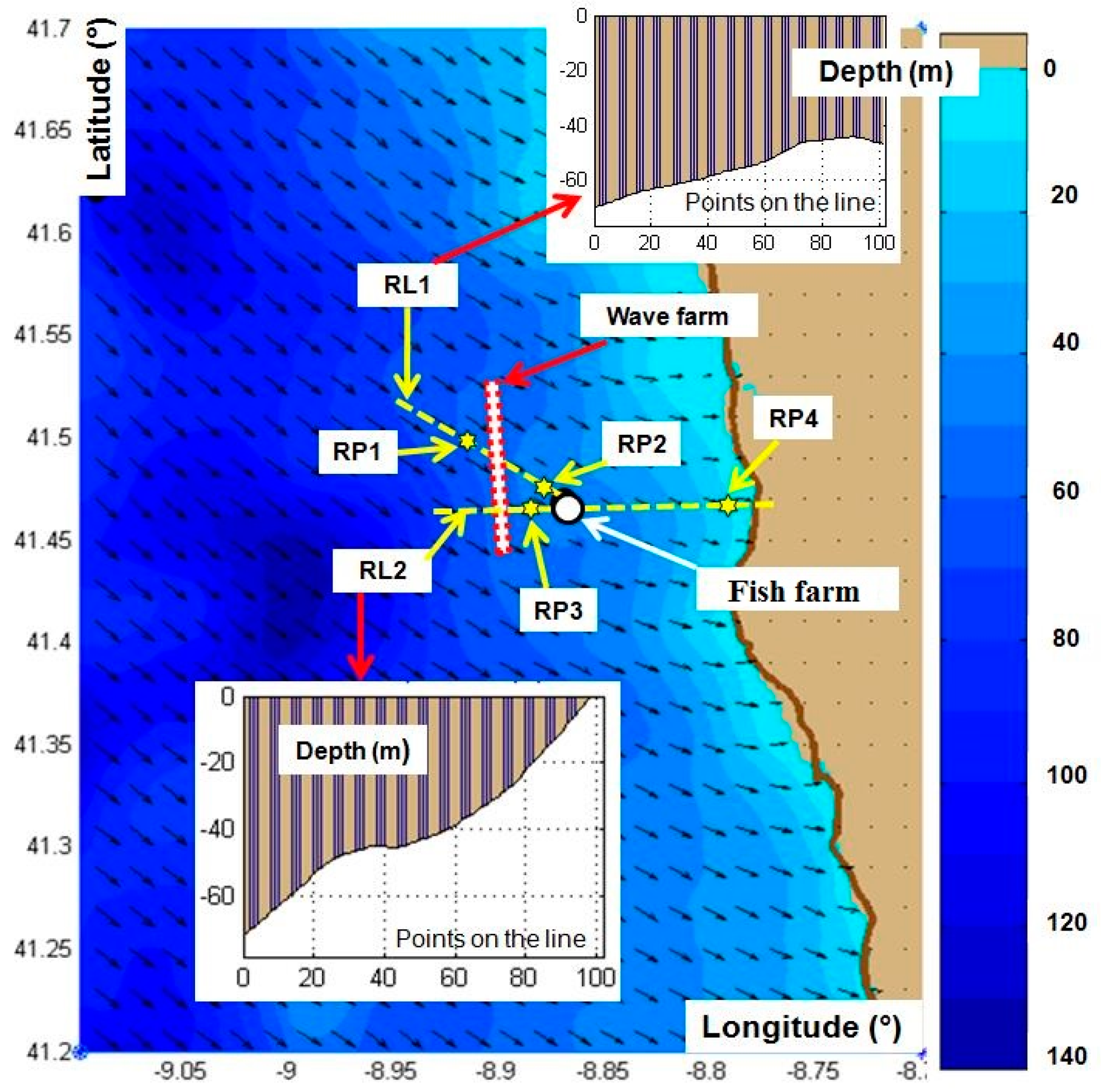
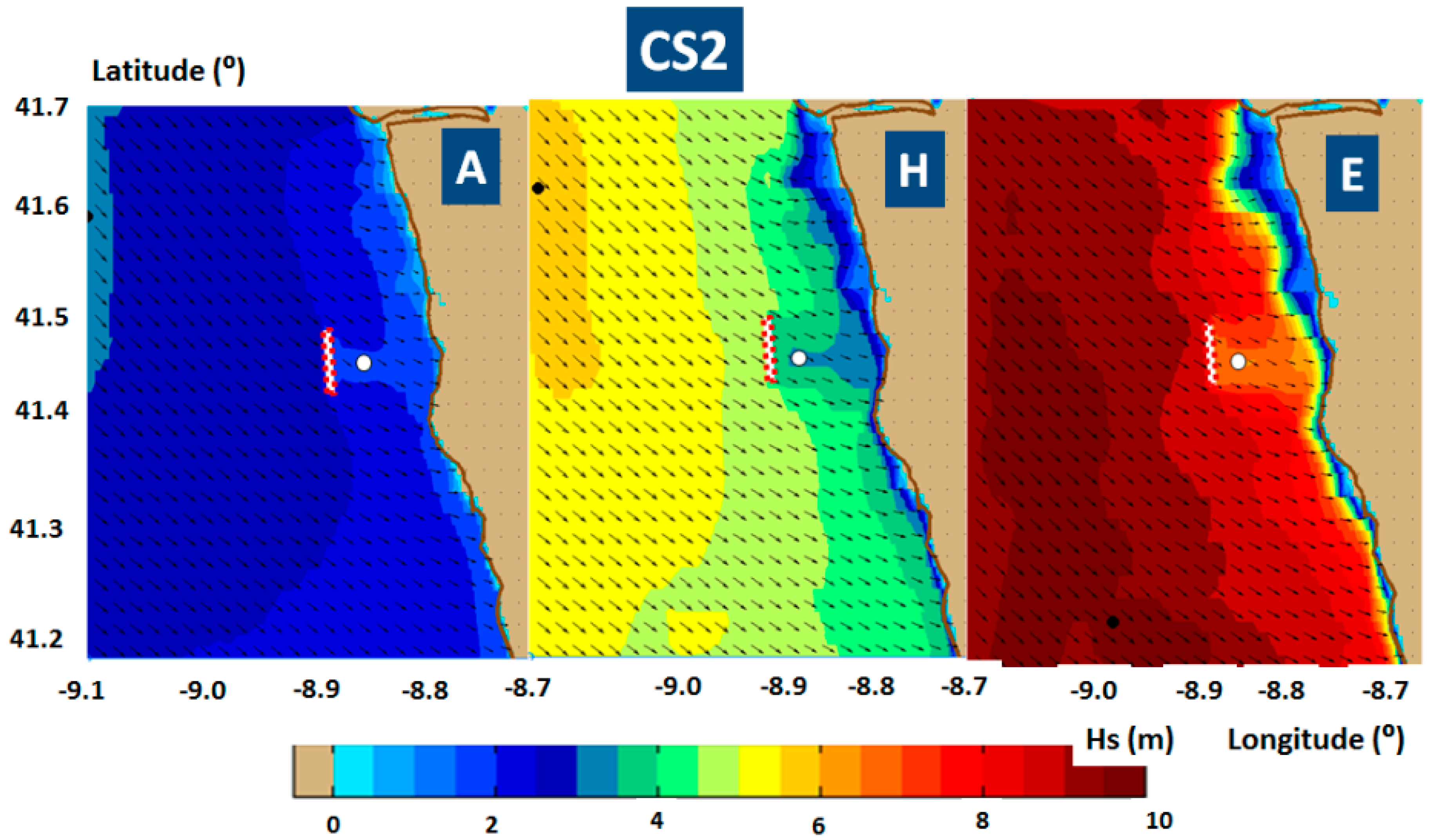
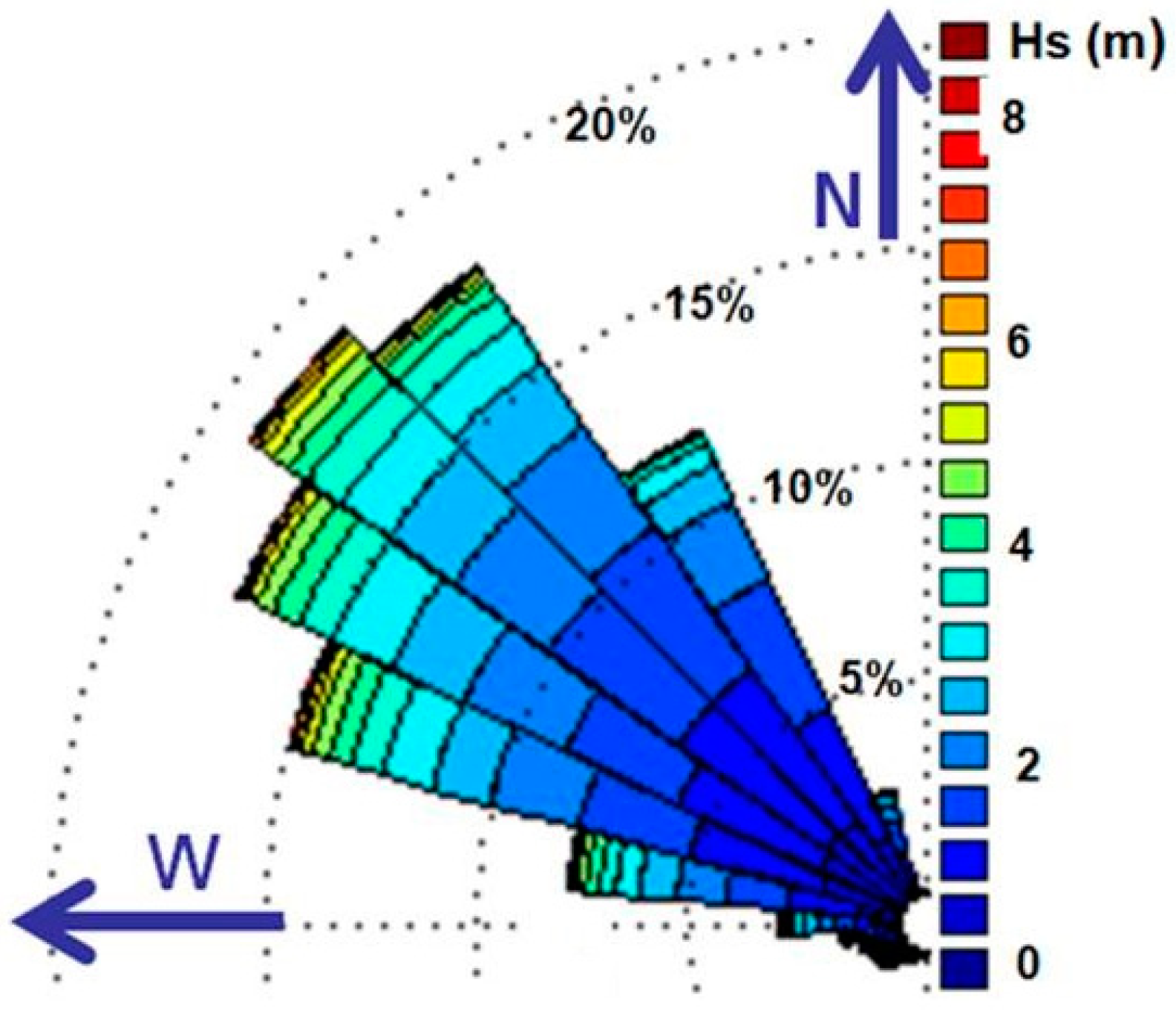
The geographical space considered in the SWAN model simulations carried out in the present work is illustrated in Figure 1, having the bathymetry of the northern side of the Portuguese coastal environment in the background. As can be seen in this figure, in the southern side of the SWAN domain, close to the offshore boundary, operates a directional buoy of Waverider type (Leixões buoy, 9.09 W, 41.2 N). Considering this data source, Figure 2 presents the Hs (significant wave height) classes distributed for each 10° directional bin in a ten-year time interval (1994–2003).

A depth analysis of the wave conditions in the area of study, including the measurements carried out at the buoy of Leixões, was performed in [24]. The bathymetric map of the SWAN computational domain is illustrated in Figure 3, where the most common pattern for the wave propagation (which is from northwest) in the target area is also suggested, with the wave vectors being represented with black arrows.

The computational characteristics and the main physical processes considered in SWAN model simulations are described in

Table 1. Description of the computational characteristics and the physical processes activated in the SWAN model simulations. X means that the process is activated and 0 means no process.

SWAN Model	Δx × Δy (°)	Δθ (°)	Mode/Scheme	Nf (fmin–fmax)	Nθ	ngx × ngy = np
Computational Characteristics	0.0025 × 0.0025	10	Stat/BSBT	34 (0.025–0.8)	36	201 × 201 = 40401
Input/Process	wave wind	gen wcap	quad	tri diff	bfric	set-up br
	X	X	X	X	X	0

. In the table, Δx and Δy indicate the resolutions considered in the geographical space, Δθ represents the resolution in the directional space, Nf indicates the number of frequencies in the spectral space, fmin and fmax are the limits of the frequency interval, Nθ represents the number of directions in the spectral space, ngx is the number of grid points in x direction, ngy is the number of grid points in y direction, and finally np indicates the total number of grid points. The meaning of the input fields and of the main physical processes activated are: wave (wave forcing), wind (wind forcing), gen (generation by wind), wcap (whitecapping process), quad (nonlinear quadruplet interactions), triad (nonlinear triad interactions), diff (diffraction), bfric (bottom friction), set-up (wave-induced set-up) and br (depth-induced wave breaking) [18]. For the physical processes the default formulations and parameters were used.

The objective of the work performed is to assess the influence of a wave energy park in terms of wave conditions over a fish farm located downwave. From this perspective, it must be highlighted that only the wave park was represented as an obstacle in the SWAN simulations. In the SWAN model the obstacle is considered sub-grid. This means that the obstacle is narrow compared to the mesh defined in the geographical space, but its length should be greater than the length of one mesh. The position of the obstacle (considered as a line) is defined by its two endpoints. Such an obstacle interrupts the wave propagation between the two grid points that are closer to its extremities. Thus, it means that, to be effective, the obstacle should cross more than one grid line. That is, it should be larger than one mesh length. The obstacle changes the waves in several ways. First, this reduces the height of the waves propagating along the obstacle, second, it causes wave reflections, and third, it induces diffraction around its ends.

The SWAN model can account in a reasonable way for the waves propagating in the vicinity of an obstacle, with the condition that the incoming waves do not have a very narrow directional spectrum. There are more mechanisms considered for the transmission of the waves [48]. The model evaluates such effect, either as the wave transmission when passing over a dam with a closed surface or as a transmission coefficient with a constant value. This last option was considered in the present work. Once activating the obstacle command, either a specular reflection or a diffuse reflection can be considered. In the first case the angle of reflection is equal to the angle of incidence, while in the second case the incident waves are scattered over the direction reflected. Thus, it can also account for the influence of the wave energy park on the incoming waves.

The values of the coefficients considered for wave transmission and diffuse reflection for the case studies that were considered in the present work are presented in

Table 2. Description of the four case studies considered (CS1–CS4).

Case Studies	CS1	CS2	CS3	CS4
	No wave farm CTr CRef 1 0	Realistic scenario CTr CRef 0.75 0.05	Optimistic scenario CTr CRef 0.5 0.1	Multi-line wave farm CTr CRef 0.25 0.2

.

The transmission (C_Tr) and the reflection (C_Ref) coefficients are formulated in terms of wave height, that is the ratio of the transmitted significant wave height (or the reflected significant wave height, respectively) over the incoming significant wave height. In the present work the values considered for these coefficients are (C_Tr = 0.9, C_Ref = 0.05). The diffraction process, which was also accounted for in the present work, was implemented in SWAN considering a phase-decoupled refraction-diffraction approach [49]. This considers the mild-slope Equation but without accounting any phase information and it is expressed as a turning rate of the wave components in the directional wave spectrum.

For evaluating, both locally and at the shoreline level, the impact induced by the wave farm, considering the above-mentioned settings and physics of the model, some simulations have been carried out with SWAN, following the most relevant wave patterns and transmission scenarios.

3. Analysis of Four Case Studies Considered for the Wave Propagation

Four different case studies (CS) were considered for this analysis and they are defined in Table 2. Thus, CS1 reflects the situation when no wave farm operates and only the fish farm is installed. CS2, which represents the so-called realistic scenario, corresponds to the situation when the wave farm operates reducing the downwave significant wave height by 25%. The optimistic scenario is denoted as CS3, when the passage through the wave farm reduces the significant wave height by 50%. Finally, the last scenario (CS4) corresponds to a highly absorbing (or multi-line wave farm), when only 25% of the significant wave height of the incoming waves is transmitted.

It should be underlined at this point that for the wide range of wave conditions that are considered in the present work, as well the elevated water levels encountered during extreme storms, the transmission and the reflection coefficients would, most likely, greatly vary. For this reason, and to cover most of the possible situations, a relatively large range of possibilities have been considered in terms of the global transmission coefficient (C_Tr) of the wave farm. Thus, the first value considered in the work, C_Tr = 1, indicates 100% transmission in terms of the parameter significant wave height and corresponds to the no farm situation. The other extremity of the range considered, the value C_Tr = 0.25, indicates only a 25% transmission in terms of significant wave height and corresponds to a highly absorber multi-line wave farm. Between them, two other situations have been considered, the so-called realistic and optimistic scenarios (C_Tr = 0.75 and C_Tr = 0.5, respectively). Some explanations regarding the selection of such transmission coefficients values are provided next. Thus, the coefficient considered for the realistic scenario is indicated by some tests performed for WECs in laboratory [32,35], which suggest for the system WaveCat a C_Tr value of 0.76. At the same time, for the DEXA (DEXA Wave Energy Converter is a Danish project related to the development of a wave energy converter) single device values in the range 0.7–0.8 can are indicated and for the array configuration about 0.8. Other results [50], from experimental data corresponding to a DEXA array, indicate C_Tr values covering the range 0.68–0.9.

Considering a simple linear superposition, [32] found that the transmission coefficient values in the case of a wave energy park with 4, 6 and 8 lines, are respectively 0.72, 0.61 and 0.52. Some similar values have been estimated for the floating buoys, which, under short period wave conditions, can absorb around 40% of the wave energy [51]. Some other experimental results, [52], show that the floating breakwaters can have values for the transmission coefficients in the range 0.28–0.65, also mentioning that, as the period of motion is closer to the natural period, the value of the transmission coefficient becomes higher. Such a case corresponds also to the WECs. Furthermore, it must be also highlighted that some other simulations carried out for WECs operating on more lines close to the Bay of Santander (Spain) and Las Glorias beach (Mexico) [34], considered transmission coefficients between 0.75 and 0.63.

For each case study, three different situations were defined by analyzing the Leixões buoy measurements. These are: (A) average wave conditions, corresponding to the real situation from 22 April 2014 3 h (h indicates the hour); (H) high wave conditions, corresponding to the time frame 8 March 2014 12 h and (E) extreme wave conditions, with the real correspondences in the time frame 14 February 2014 19 h. For each situation defined (A, H, E), the values of the main wave parameters together with the wind conditions, used as boundary conditions in SWAN simulations, are given in

Table 3. Values of the main wave and wind parameters defined for the north western (offshore) boundary of the SWAN computational domain. A—average wave conditions, H—high wave conditions, E—extreme wave conditions.

Energetic Situation	Hs (m)	Tp (s)	Dir (°)	DSPR (°)	Vw (m/s)	Dw (°)
A—average	3.04	7.1	314.6	22.7	8.2	311.2
H—high	5.52	11.4	317.1	28.3	11.6	307.8
E—extreme	9.1	14.2	312.6	32.4	14.3	316.3

.

In Table 3 and

Table 4. Values of the most relevant wave parameters in the four reference points considered (RP1, depth 54.5 m; RP2 depth 44.8 m; RP3, depth 47.1 m and RP4, depth 9.9 m).

Case Study	Energetic Situation	Reference Point	Hs (m)	Hsw (m)	Tp/Tm (s)	Dir (°)	PDir (°)	Wlen (m)	DSPR (°)
CS1	A	RP1	2.54	0.23	5.7/7.1	306.5	315.0	37.9	29.5
		RP2	2.50	0.23	5.7/7.1	303.4	315.0	37.5	29.6
		RP3	2.51	0.23	5.7/7.1	303.6	315.0	37.9	30.3
		RP4	1.8	0.17	5.2/7.1	282.8	295.0	26.8	23.3
	H	RP1	4.80	3.52	8.4/10.6	301.3	315.0	81.1	27.8
		RP2	4.67	3.42	8.3/10.6	298.3	305.0	78.6	27.1
		RP3	4.69	3.42	8.3/10.6	298.4	305.0	78.9	27.9
		RP4	3.42	2.49	8.0/10.6	276.6	285.0	54.9	17.2
	E	RP1	8.91	7.32	9.9/14.4	300.8	315.0	113.5	29.2
		RP2	8.80	7.20	9.9/14.4	298.1	305.0	111.0	27.5
		RP3	8.77	7.14	9.9/14.4	298.4	305.0	110.5	28.2
		RP4	5.04	3.95	9.6/14.4	273.9	285.0	76.9	14.9
CS2	A	RP1	2.54	0.23	5.7/7.1	306.6	315.0	38.0	29.6
		RP2	1.95	0.17	5.4/7.1	305.7	315.0	31.7	30.7
		RP3	1.95	0.17	5.4/7.1	305.0	315.0	31.6	31.5
		RP4	1.61	0.14	5.0/7.1	284.3	295.0	24.0	25.0
	H	RP1	4.80	3.52	8.4/10.6	301.4	315.0	81.1	27.9
		RP2	3.59	2.59	8.0/10.6	299.7	305.0	66.5	27.9
		RP3	3.59	2.58	7.9/10.6	299.3	305.0	66.3	28.8
		RP4	3.02	2.16	7.6/10.6	277.5	285.0	49.0	18.9
	E	RP1	8.95	7.32	9.9/14.4	300.9	315.0	113.5	29.3
		RP2	6.85	5.44	9.3/14.4	300.1	305.0	92.6	28.7
		RP3	6.81	5.37	9.2/14.4	300.1	305.0	91.7	29.5
		RP4	4.77	3.7	9.3/14.4	275.5	285.0	71.0	16.2
CS3	A	RP1	2.55	0.23	5.7/7.1	306.7	315.0	38.0	30.0
		RP2	1.41	0.12	5.0/7.1	311.3	315.0	23.9	32.4
		RP3	1.40	0.12	4.9/7.1	309.1	305.0	23.3	33.9
		RP4	1.46	0.12	4.7/7.1	286.2	295.0	21.4	26.7
	H	RP1	4.81	3.53	8.4/10.6	301.5	315.0	81.2	28.5
		RP2	2.52	1.76	7.3/10.6	303.3	315.0	49.1	29.7
		RP3	2.49	1.73	7.3/10.6	301.7	305.0	48.2	30.8
		RP4	2.64	1.84	7.2/10.6	278.6	285.0	42.8	21.0
	E	RP1	9.0	7.33	9.9/14.4	301.0	315.0	113.6	31.0
		RP2	4.90	3.69	8.3/14.4	305.3	315.0	68.6	31.1
		RP3	4.85	3.62	8.2/14.4	304.4	305.0	67.0	32.3
		RP4	4.48	3.39	8.9/14.4	277.2	285.0	63.7	18.0
CS4	A	RP1	2.55	0.23	5.7/7.1	307.2	315.0	38.0	31.6
		RP2	0.95	0.07	4.1/7.1	326.0	345.0	15.0	33.0
		RP3	0.91	0.06	3.9/7.1	322.1	345.0	13.7	37.8
		RP4	1.35	0.10	4.5/7.1	288.0	305.0	19.5	28.3
	H	RP1	4.84	3.56	8.3/10.6	302.0	305.0	78.5	30.7
		RP2	1.57	0.97	5.7/10.6	316.0	335.0	25.5	32.9
		RP3	1.50	0.92	5.4/10.6	311.4	345.0	23.4	36.6
		RP4	2.36	1.57	6.6/10.6	280.1	295.0	36.0	23.5
	E	RP1	9.0	7.38	10.0/14.4	301.5	315.0	113.9	31.8
		RP2	3.1	2.01	6.5/14.4	321.0	335.0	39.7	33.7
		RP3	3.08	1.91	6.3/14.4	319.0	345.0	37.4	36.9
		RP4	4.17	3.05	8.3/14.4	279.1	295.0	56.1	20.1

Hs represents the significant wave height, Tp is the peak wave period and Dir the mean wave direction, defined by their standard definitions as given in [26]. DSPR is the directional spreading of the waves, or directional standard deviation, and it can be associated with directional width of the spectrum [53]. Finally, V_w and D_w are the wind velocity and direction, respectively.

For evaluating the local changes and the beach response for each situation considered, two reference lines (RL1, RL2) and four reference points (RP1, RP2, RP3 and RP4, where the first two are located on RL1 and the last two on RL2) were defined and their positions are illustrated in Figure 3.

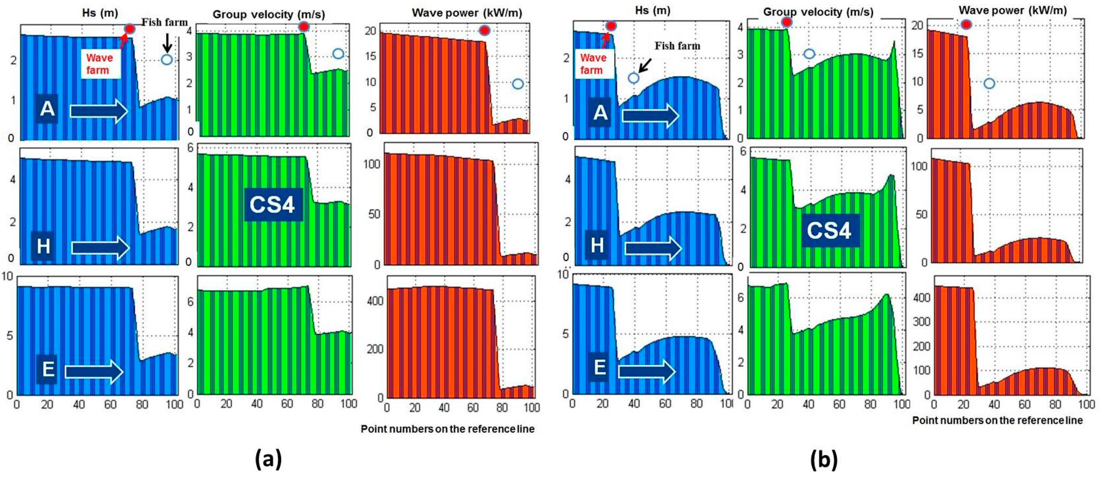
The first reference line (RL1) has the length of about 12 km and follows the most expected mean wave direction offshore the wave farm (northwest). Following the variations of the most relevant wave parameters along this line, it can be noticed that the influence of the wave energy park on the downwave climate, especially the wave’s attenuation just in front the fish farm. The second reference line (denoted as RL2) has a length of about 20 km and it is approximately normal to the shore. Following the variations of the most relevant wave parameters along this line, not only can the wave decrease induced by the wave energy park in front of the fish farm be noticed, but also the direct impact on the wave conditions at the shoreline level. The variations of the water depth along the two reference lines, considering 100 equally spaced points, are also represented in Figure 3.

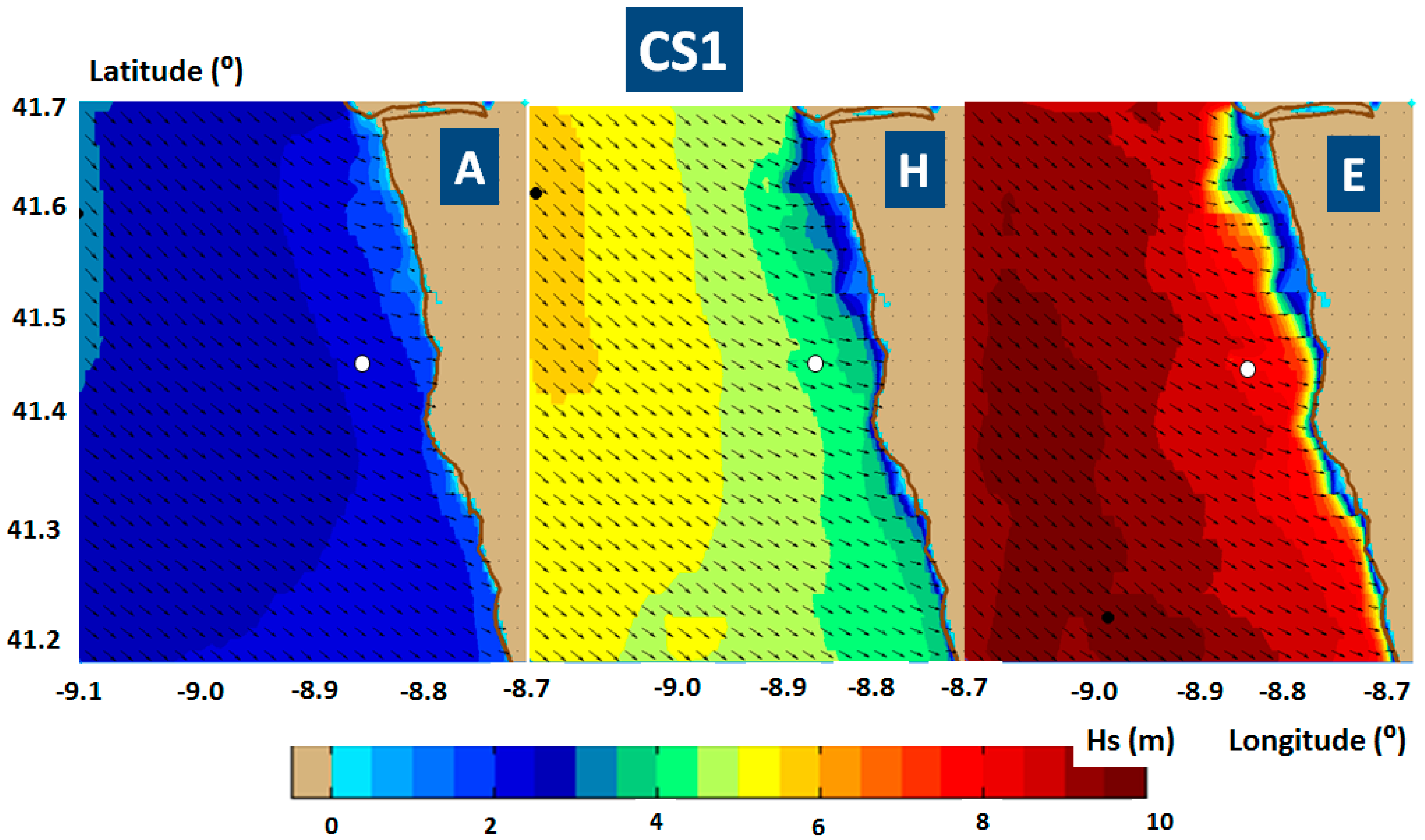
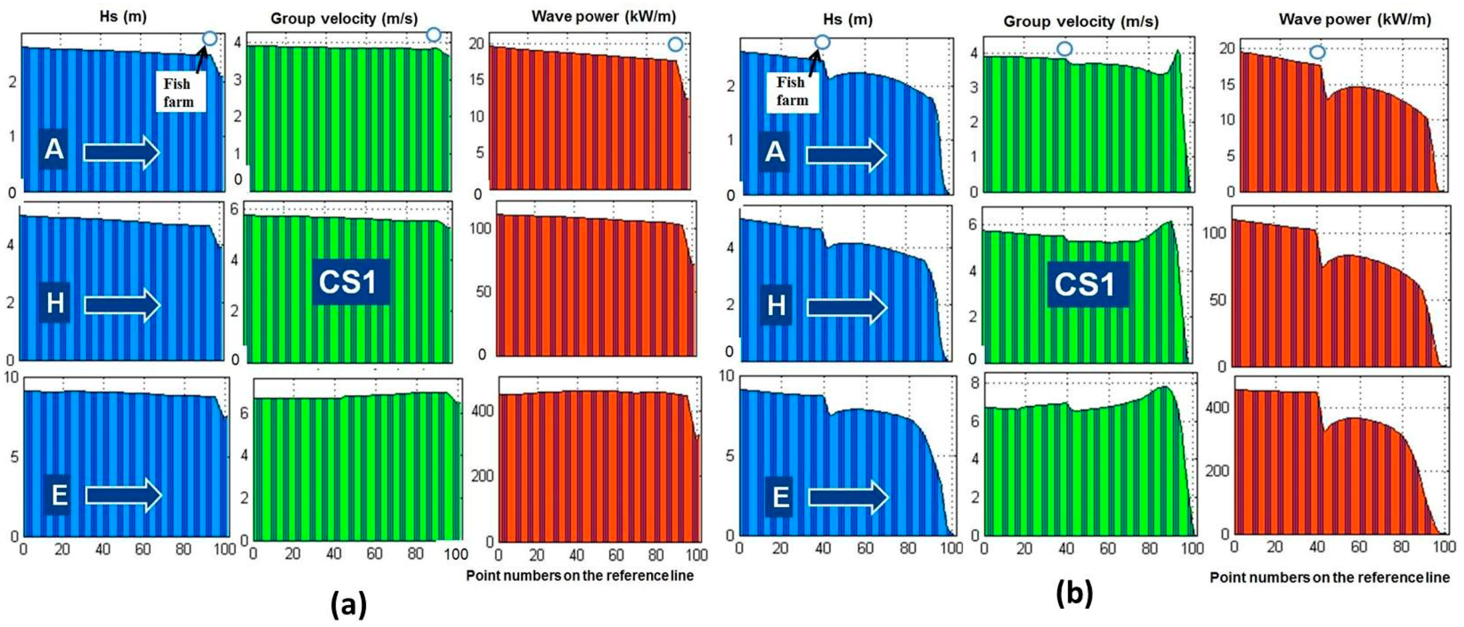
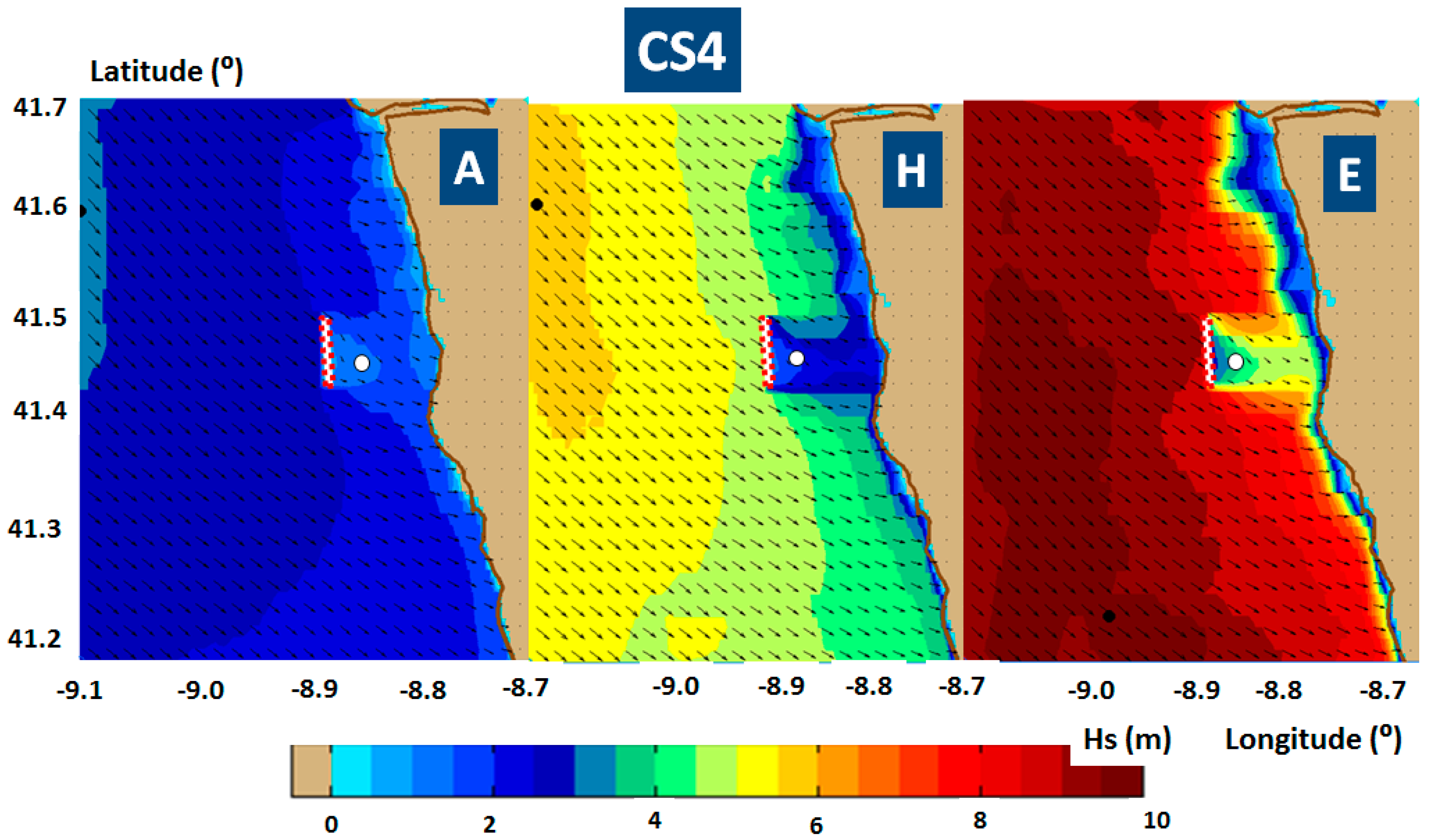
For CS1, Figure 4 illustrates in background the significant wave height scalar fields, as resulted from the SWAN model simulations, corresponding to the three different energetic situations considered (A, H and E). The wave vectors are represented in the foreground, with Hs as magnitude and the mean wave direction. 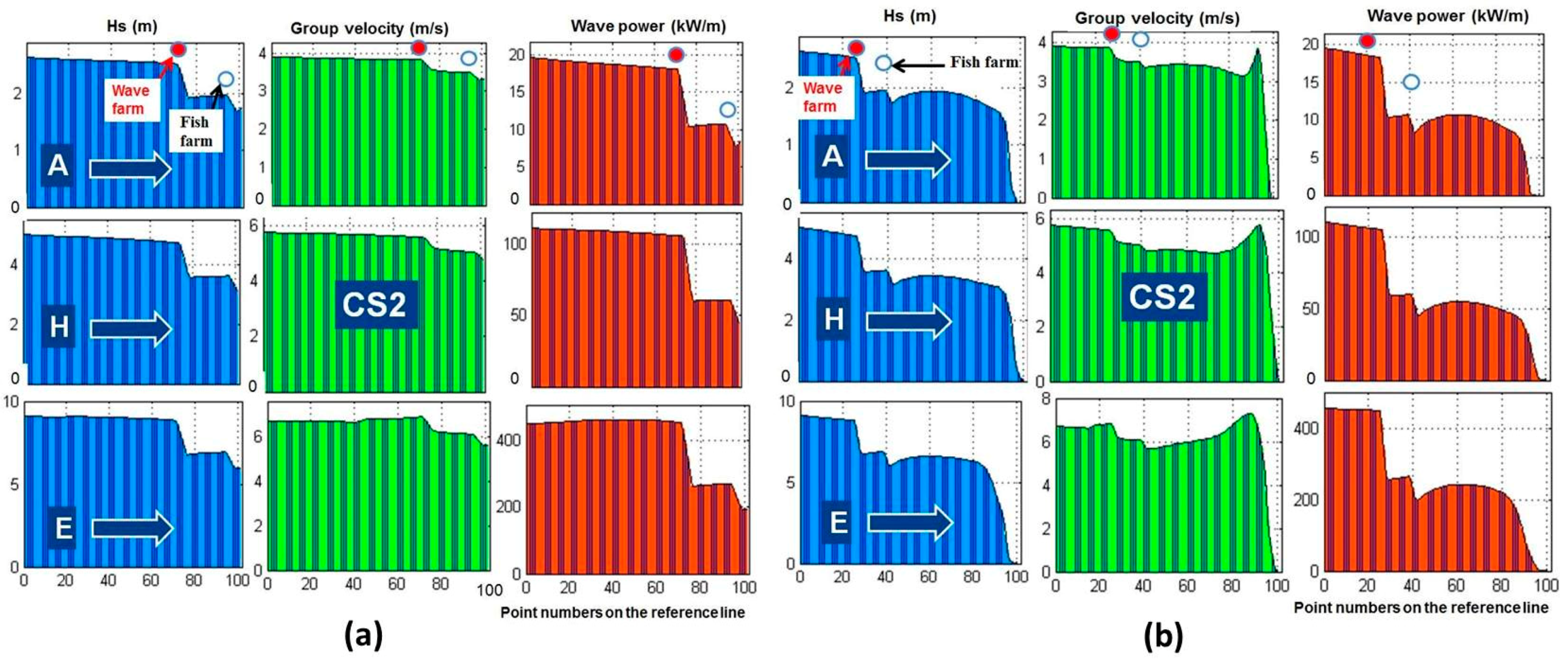The variations along the two reference lines of the significant wave height (Hs), group velocity (C_g) and wave power over a meter of wave front (P_W) are shown in the Figure 5. 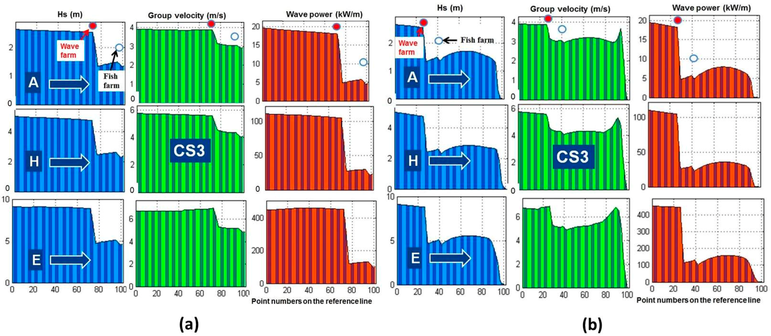For CS2 the corresponding results are presented in Figure 6 and Figure 7, for CS3 in Figure 8 and Figure 9 while for CS4 in Figure 10 and Figure 11.

In SWAN the energy transport components distributed along one meter the of the wave front (expressed in W/m) are estimated with the next relationships:

$$P_{wx}=\rho g\iint C_{gx}E\left(\sigma ,\theta \right)d\sigma d\theta$$

(4)

$$P_{wx}=\rho g\iint C_{gx}E\left(\sigma ,\theta \right)d\sigma d\theta$$

(5)

where x, y are the problem coordinates (in the case of spherical coordinates, x axis represents the longitude and y axis the latitude), and in the absence of currents C_gx, C_gy represent the group velocity components and express the velocities of the wave energy propagation in the geographical space, as follows:

$$c_x=\frac{dx}{dt}, c_y=\frac{dy}{dt}$$

(6)

Thus, the wave power in absolute value, results:

$$P_w=\sqrt{P_{wx}^2+P_{wy}^2}$$

(7)

The values of some relevant wave parameters in the four reference points considered, for the four cases, are given in Table 4.

Besides the main wave parameters defined before (Hs, Tp, Dir and DSPR), some additional wave parameters were also evaluated. These are: Hsw (significant wave height of the swell, this representing the part of the significant wave height which is associated with the low frequency part of the spectrum), Tm (mean absolute wave period), PDir (peak direction) and Wlen (wave length). All these spectral parameters are evaluated by the SWAN model considering their standard definitions [37].

4. Analysis of the Results and Discussion

As the results presented in Figure 4 and Figure 5 clearly indicate, the fish farm has a small local impact on wave propagation. Moreover, this is completely attenuated at shoreline level, for all the situations considered. Nevertheless, it must be highlighted that SWAN model simulations have been also carried out without including the influence of the fish farm, but the results were not represented in a separate figure due to the similar results at the coastline level when the fish farm is considered, whose effect on the wave field is only local. The next discussions will be focused first on the local impact, especially on the sheltering effect of the wave energy farm to the fish farm located downwave, and second the expected impact on the wave conditions at the shoreline level.

4.1. Influence of the WECs on the Fish Farm

Figure 6, Figure 7, Figure 8, Figure 9, Figure 10 and Figure 11 indicate very clearly that the wave farm considered in the present work would induce immediately downwave a significant shadow effect that would protect the fish farm. By comparing the results presented in Figure 4 with those from Figure 6, Figure 8 and Figure 10, which provide information concerning the spatial distributions in the geographical space of the significant wave height fields, it can be noticed that a large wave farm operating upwave of the fish farm would have a strong local effect by decreasing drastically the significant wave height. The same conclusion is suggested by comparing the results illustrated in Figure 5 with those from Figure 7, Figure 9 and Figure 11. As the figures show, the values of all the parameters (Hs, Cg and P_w) are substantially decreased immediately after the wave farm, leading to an obvious sheltering effect for the fish farm.

A more detailed analysis is provided by comparing the values of the main wave parameters in the reference point RP1 (located on the reference line RL1 upwave of the wave farm) with those in the reference points RP2 (located on the same reference line downwave the energy farm) and RP3 (located on the reference line RL2 downwave the energy farm). The positions of these reference lines and reference points are illustrated in Figure 3 while the values of the main wave parameters analyzed are presented in Table 4.

The differences of the wave parameters values from RP1 to RP2 and RP3 increase as the sea states become more severe (from A situation to E) and the wave farm absorbs more energy (from CS2 to CS4). Between the two downwave reference points (RP2 and RP3), in general, there are no significant differences in the parameters values. For significant wave height (Hs) (differences in the range 0.03 m (situation A in CS1) to 5.9 m (situation E in CS4)), significant height of the swell (Hsw) (differences in the range 0.2 m (situation A in CS1) to 5.4 m (situation E in CS4)), mean period (Tm) (differences in the range 0.1 s (situation H in CS1) to 3.5 s (situation E in CS4), peak period (Tp) (remains the same) and wave length (Wlen) (differences in the range 0.4 m (situation A in CS1) to 74 m (situation E in CS4)), there is a reduction of the values downwave the wave farm, while this reduction, although small, is higher in the RP3. For DSPR (differences in the range 0.1 m (situation A in CS1) to 6.2 m (situation A in CS4)) the tendency is to increase, and again the RP3 presents the higher increment. In terms of mean wave direction (Dir), the behavior change depending on the case study. For CS1 and CS2 the differences between RP1 to RP2 and RP3 are smaller, but the tendency is the wave direction go further south (the values slightly decrease, in the range of 1° to 3°). For CS3 and CS4 the tendency is to go further north (the values increase, in the range of 1° to 20°), and this is more accentuated in RP2.

Considering the classification mentioned in the Introduction, the degree of fish farm exposure passed from class 4 (high exposure) to class 3 (medium exposure) in the case of CS2 and CS3 for the average wave conditions (A). For CS4, in the same conditions (energetic situation A), it passed from class 4 (high exposure) to class 2 (moderate exposure). Although the significant reduction of the significant wave height for CS2 in the situation H and E and for CS3 and CS4 in situation E, the degree of exposure remains in the same class, which is 5 (extreme exposure). Finally, in the CS3 and CS4 for situation H, it passed from class 5 to class 4 and class 3 respectively.

4.2. Influence of the WECs on the Coast

Regarding the shoreline impact induced by the presence of the wave energy park, the variation of the wave parameters Hs, Cg and Pw along the reference line RL2, that has the offshore extremity upwave of the wave farm and its nearshore extremity located at the shoreline level (almost perpendicular to the coast) is presented in Figure 5b, Figure 7b, Figure 9b and Figure 11b.

More quantitative information in relationship to the wave park impact in the shoreline dynamics (and especially on the wave climate close to the shore) is given by the analysis of the main wave parameters in the reference point RP4, which is located at about 9.9 m water depth and thus is almost always located before the start of the breaking process in any of the three situations considered (A, H or E).

Thus, for the situation (A), when the offshore significant wave height is about 2.54 m (in RP1 in the case of no wave farm, CS1), in RP4 the values of this parameter are 1.8 m (CS1), 1.61 m (CS2), 1.46 m (CS3) and 1.35 m (CS4). In relative terms, the nearshore Hs decreases in relationship with CS1 are: 10.6% for CS2, 18.8% for CS3 and 25% for CS4. In terms of significant wave height of the swell, the relative decreases are: 17.6% for CS2, 29.4% for CS3 and 41.2% for CS4. The mean wave direction in RP4 is 282.8° for CS1 and increases with 1.5° in CS2, with 3.4° in CS3 and with 5.2° in CS4. A slight decrease of the wavelength can be noticed from CS1 to CS4, while the DSPR increases with about 2° from one case study to another.

For the situation (H), the offshore significant wave height is about 4.8 m (in RP1 in the case of no wave farm, CS1). The values of the same wave parameter in RP4 are 3.42 m (CS1), 3.02 m (CS2), 2.64 m (CS3) and 2.36 m (CS4). In relative terms, the nearshore Hs decreases in relationship with CS1 are: 11.7% for CS2, 22.8% for CS3 and 31% for CS4. In terms of significant wave height of the swell, the relative decreases for this energetic situation are: 13.2% for CS2, 26.1% for CS3 and 36.9% for CS4. The mean wave direction in RP4 is 276.6° for CS1 and increases with 0.9° in CS2, with 2° in CS3 and with 3.5° in CS4. The behavior of the parameters wave length and DSPR remains almost the same as in the previous situation (A).

For the extreme wave situation considered (E), the offshore significant wave height is about 8.91 m (in RP1 in the case of no wave farm, CS1)). The values of this parameter in RP4 are 5.04 m (CS1), 4.77 m (CS2), 4.48 m (CS3) and 4.17 m (CS4). In relative terms, this time the nearshore Hs decreases in relationship with CS1 are: 5.4% for CS2, 11.1% for CS3 and 17.3% for CS4. In terms of significant wave height of the swell, the relative decreases for this energetic situation are: 6.3% for CS2, 14.2% for CS3 and 22.8% for CS4. The mean wave direction in RP4 is in this case 273.9° for CS1 and increases with 1.6° in CS2, with 3.3° in CS3 and with 5.2° in CS4. The tendency remains the same for the wavelength and for the DSPR.

The above results show that, in terms of significant wave height, the relative nearshore impact of the wave farm increases from average to high-energy situations but decreases when going to extreme situations. This means that the wave farm considered will induce a relevant coastal impact, reflected by a relative decrease in terms of the nearshore significant wave height with more than 10%. Such a decrease can be noticed even in the case of the realistic scenario (CS2) and this reduction is enhanced as the energy absorption proprieties of the wave farm are increased. The coastal impact of the wave farm in the central part of the Portuguese continental nearshore was also analyzed in [27,28] and the results are in line with those presented above. Moreover, as discussed in [28], since the wave farm modifies both the significant wave height and the wave direction, the changes in the nearshore currents are sometimes enhanced and thus the wave energy park can play a determinant role in controlling the shoreline dynamics.

5. Conclusions

The target area considered in the present study is the coastal environment of Aguçadoura, situated in the northern part of the Portuguese coastal environment. This is a very representative location from the point of view of the ocean energy extraction, in such a way that the world’s first wave farm was tested here in 2008. The possibility to install a fish farm downwave of the energy farm with the purpose of being sheltered from the wave conditions was analyzed. This is a good strategy to consider, while the wave farm producing electricity is simultaneously protecting the fish farm, which in turn increases the viability of aquaculture offshore and decreases the possibility of the structures being damaged.

From this perspective, the local and coastal impact on the wave conditions of the ocean farm was assessed, considering various transmission scenarios, and performing simulations with a wave modelling system, based on the SWAN third-generation spectral phase averaged model. The results showed that the wave farm provides a sheltering effect to the fish farm, increasing in this way its safety. There is an improvement related to the classification of the degree of equipment exposure, e.g., for CS2 in the situation of average wave condition (A) it passed from class 4 (high exposure) to class 3 (medium exposure).

Besides this, the results coming from this work also indicate that a relative decrease in terms of significant wave height is expected at shoreline level, depending on the characteristics of the wave farm, and this might represent a viable solution for coastal protection.