Article

A Stochastic Inexact Robust Model for Regional Energy System Management and Emission Reduction Potential Analysis—A Case Study of Zibo City, China

1
School of Energy and Environmental Engineering, University of Science and Technology Beijing, Beijing 100083, China
2
The Vehicle Pollution Prevention and Control Center of Jinan, Jinan Environmental Protection Bureau, Jinan 250099, Shandong, China
3
Environmental Systems Engineering Program, Faculty of Engineering, University of Regina, Regina, SK S4S 0A2, Canada
4
School of Economics and Management, Beijing University of Technology, Beijing 100124, China
*
Author to whom correspondence should be addressed.
Energies 2018, 11(8), 2108; https://doi.org/10.3390/en11082108
Submission received: 4 July 2018 / Revised: 23 July 2018 / Accepted: 3 August 2018 / Published: 13 August 2018
(This article belongs to the Special Issue Optimisation Models and Methods in Energy Systems)

Abstract

:
In this study, in order to improve regional energy system adjustment, a multistage stochastic inexact robust programming (MSIRP) is proposed for electric-power generation planning and structure adjustment management under uncertainty. Scenario-based inexact multistage stochastic programming and stochastic robust optimization were integrated into general programming to reflect uncertainties that were expressed as interval values and probability distributions in the objective function and constraints. An MSIRP-based energy system optimization model is proposed for electric-power structure management of Zibo City in Shandong Province, China. Three power demand scenarios associated with electric-power structure adjustment, imported electricity, and emission reduction were designed to obtain multiple decision schemes for supporting regional sustainable energy system development. The power generation schemes, imported electricity, and emissions of CO2 and air pollutants were analyzed. The results indicated that the model can effectively not only provide a more stable energy supply strategies and electric-power structure adjustment schemes, but also improve the balanced development between conventional and new clear power generation technologies under uncertainty.

1. Introduction

Rapid power consumption increment, increasing deterioration of environmental quality, and imperfect energy system management have led to unsustainable energy resources exploitation and utilization, unreasonable electric-power structure, and serious environmental issues [1,2,3]. In order to search effective and suitable energy development strategies for regional condition, energy system management and planning has become a priority for many countries and regions. However, multiple forms of uncertain information are involved in energy system management and the related social-economic factors and/or technical-economic parameters, causing a variety of complexities in decision support and policy analysis for regional energy planning [4]. In addition, such complexities would pose great challenges in formulating more scientific and reasonable development strategies for decision-makers, and have serious impact on the effectiveness of energy supply schemes. Therefore, it is desirable to develop effective uncertain optimization models/techniques for energy system management and the related decision analysis.
Previously, a great number of inexact programming approaches were proposed for helping energy system planning and management in different regional scales [5,6,7,8,9,10,11,12,13,14]. For example, Cai et al. (2009) advanced an interval parameter interactive decision support system for energy system management under reflecting uncertainties as interval values [15]. Li et al. (2010) proposed an inexact fuzzy multistage stochastic energy system management model for supporting regional electric-power generation and capacity planning, where interval parameter programming, mixed integer linear programming, multistage stochastic programming, and fuzzy linear programming were incorporated into a general optimization framework [16]. Li et al. (2011) proposed a fuzzy stochastic energy system optimization model associated with renewable energy development and greenhouse gas mitigation, where the uncertainties in the objective and constraints were expressed as fuzzy interval functions, interval values, and discrete probability distributions [17]. Huang et al. (2017) developed an inexact fuzzy stochastic chance-constrained programming for evacuation management of nuclear power plant, where interval parameter programming and fuzzy stochastic chance-constrained programming were integrated into a general framework for dealing with uncertainties [18]. Sheikhahmadi et al. (2018) proposed a risk-based two-stage stochastic programming for microgrid system operation management, where two-stage stochastic programming was to reflect uncertainties of renewable energy, and conditional value at risk index was used to avoid the system risk [19].
Among these methods, scenario-based interval multistage stochastic programming, as a hybrid method of interval parameter programming and scenario-based multistage stochastic programming, could deal with uncertainties presented as interval numbers and random distributions, and have been widely applied in energy system management [20,21,22]. For example, Xie et al. (2010) advanced an inexact fixed-mix multistage stochastic programming for long-term greenhouse gas emission reduction management in a regional scale energy system, where the fixed probability multistage stochastic programming and interval-parameter programming were integrated for expressing uncertainties in energy system management problems [23]. Wu et al. (2015) proposed an integrated method with interval-parameter programming, chance-constraint programming, and multistage stochastic programming for the coupled biomass–municipal solid waste power system operation management, which could reflect uncertainties as interval information and random distributions over a multistage context [24]. Golari et al. (2016) presented a production-inventory planning model in a multi-plant manufacturing system powered with onsite and grid renewable energy, where multistage stochastic programming was used to reflect system dynamic and uncertainties [25]. Fu et al. (2017) advanced an interval multistage fuzzy-stochastic programming for regional electric-power system management under considering environmental quality constraints, where interval-parameter programming, multistage stochastic programming, and fuzzy probability distribution was integrated to reflect the uncertain information and dynamic variation in the energy system [26]. Wang et al. (2018) developed multistage joint-probabilistic left-hand-side chance-constrained fractional programming for electric-power system planning considering climate change mitigation [27].
Although scenario-based inexact multistage stochastic programming had been successfully applied in many fields, it could not directly and effectively avoid the risk of random events, and the limitations would pose threats to system stability. Based on this point, stochastic robust optimization (SRO) is proposed for solving the problems through introducing the risk-aversion attitude into optimization models and obtaining robust solutions for stochastic system management [28,29,30]. The methods that coupled with the scenario-based inexact multistage stochastic programming and SRO have been used in solving many energy and environmental problems, such as water resources allocation, electric-power generation, and water/air quality management. For example, Chen et al. (2013) developed an interval robust-optimization model for CO2 emission reduction management in energy systems, where the robustness measures were introduced to examine whether the second-stage cost variability could meet the expected levels or not [31]. Xie et al. (2014) proposed an inexact stochastic risk-aversion model for electric-power structure adjustment and pollutant emission management, where interval-parameter programming, stochastic robust optimization, and multistage stochastic programming were integrated to address system uncertainties [32].
Therefore, the aim of this study is to formulate a multistage stochastic inexact robust programming (MSIRP) model to support regional electric-power system management coupled with pollutant mitigation constraints and power structure adjustment requirements in Zibo City, China. The method could not only reflect multiple uncertainties expressed as interval values and probability distribution, but also make a tradeoff between system risk and cost according to the decision-makers’ attitudes. The modeling results will be helpful for local decision-makers to choose cost–risk electric-power generation schemes, and obtain reasonable electric-power structure adjustment strategies. The rest structure organization of this paper is provided as follows. The development process and solution algorithm of multistage stochastic inexact robust programming (MSIRP) is introduced in Section 2. The overview of the energy system of Zibo City are described, and a MSIRP-based energy structure adjustment model is proposed in Section 3. The obtained results and deep discovery of the case study are analyzed and discussed in Section 4. The main conclusions are presented in Section 5.

2. Methodology

In regional energy systems, dynamic characters, discrete probability distributions, intervals information, and policy implications were addressed through scenario-based inexact multistage stochastic programming, and SRO could effectively handle the system risk. The modeling framework of the MSIRP could obtain applicable and reasonable solutions under different random scenarios corresponding to power generation targets for decision-makers in order to support the energy system development in the future.

2.1. Inexact Scenario-Based Multistage Stochastic Programming

In the scenario-based multistage stochastic programming, the probabilities p t k ( t = 1 , 2 , , T ; k = 1 , 2 , , K t , ) of the stochastic event have predefined values, and the parameters without probability can be reflected as interval values. Thus, the scenario-based inexact multistage stochastic programming can be expressed as follows [33,34]:
M i n f ± = t = 1 T j = 1 n 1 c j t ± x j t ± + t = 1 T j = 1 n 1 k = 1 K t p t k d j t ± y j t k ± ,
subject to
j = 1 n 1 a r j t ± x j t ± b r t ± , r , t
j = 1 n 1 a i j t ± x j t ± + j = 1 n 1 e i j t ± y j k t ± w ˜ i t k ± , i , t , k
x j t ± 0 , t , j = 1 , 2 , , n 1
y j k t ± 0 , t , k , j = 1 , 2 , , n 1
where p t k is the probability for scenario k in period t; for each period t, the total number of scenarios is denoted as K t , and k = 1 K t p t k = 1 ; and w ˜ i k t ± represents the random parameter in the model associated with the occurrence probability p t k in period t. x j t ± denotes the first-stage variables that have to be determined before the random event occurrence; and y j k t ± are the second-stage variables that have to be decided for making a recourse actions to fulfil validity of the decision-making after the random event occurrence.

2.2. Inexact Multistage Stochastic Robust Programming

The proposed inexact scenario-based multistage stochastic programming can effectively reflect stochastic information, interval values, and dynamic feature by means of discrete random variables in long-term planning problems. However, Model (1) could not effectively reflect the system risk introduced by random information, that directly affect the feasibility and reliability of the proposed model. SRO is an effective choice for solving such problems, and it can be introduced into Model (1), that leads to a multistage stochastic inexact robust programming (MSIRP) as follows [32]:
M i n f ± = t = 1 T j = 1 n 1 c j t ± x j t ± + t = 1 T j = 1 n 2 k = 1 K t p t k d j t ± y j t k ± + ω t = 1 T j = 1 n 2 k = 1 K t p t k | d j t ± y j t k ± j = 1 n 2 k = 1 K t p t k d j t ± y j t k ± |   ,
subject to
j = 1 n 1 a r j t ± x j t ± b r t ± , r , t
j = 1 n 1 a i j t ± x j t ± + j = 1 n 1 e i j t ± y j k t ± w ˜ i t k ± , i , t , k
x j t ± 0 , t , j = 1 , 2 , , n 1
y j k t ± 0 , t , k , j = 1 , 2 , , n 1
where the non-negative factor ω denotes a trade-off weight coefficient; and | d j t ± y j t k ± j = 1 n 2 k = 1 K t p t k d j t ± y j t k ± | is a variability measure for reflecting the multistage recourse costs. The objective of Model (6) is a nonlinear function, and according to [35,36], the model can be converted into a linear programming model as follows:
M i n f ± = t = 1 T j = 1 n 1 c j t ± x j t ± + t = 1 T j = 1 n 1 k = 1 K t p t k d j t ± y j t k ± + ω t = 1 T j = 1 n 1 k = 1 K t p t k ( d j t ± y j t k ± j = 1 n 1 k = 1 K t p t k d j t ± y j t k ± + 2 θ j k t ± ) ,
subject to
d j t ± y j t k ± j = 1 n 1 k = 1 K t p t k d j t ± y j t k ± + θ j k t ± 0 , k , j = 1 , 2 , , n 1
j = 1 n 1 a r j t ± x j t ± b r t ± , r , t
j = 1 n 1 a i j t ± x j t ± + j = 1 n 1 e i j t ± y j k t ± w ˜ i t k ± , i , t , k
x j t ± 0 , t , j = 1 , 2 , , n 1
y j k t ± 0 , t , k , j = 1 , 2 , , n 1
where, through introducing the slack variable θ j k t ± , the objective can be transferred into a linear function as well as generate a specific control constraint (12). For Model (11), the first-stage variables x j t ± are considered/inputted as interval values with the lower and upper bound, and this cannot be directly solved using the existing methods. In this study, let μ j t be a decision variable, μ j t [ 0 , 1 ] ; Δ x j t = x j t + x j t , the first-stage variable x j t = x j t + μ j t Δ x j t , and μ j t are intermediate decision variables for obtaining an optimized target values of the first-stage to support the related policy analyses [32]. According to [37], the MSIRP model can be transformed into two linear submodels, and the submodel corresponding to f can be firstly transformed as follows (assume that c j t ± 0 , w ^ i t k + > 0 , b r t ± > 0 , and f ± > 0 ):
M i n f = t = 1 T j = 1 n 1 c j t ( x j t + μ j t Δ x j t ) + t = 1 T k = 1 K t p t k ( j = 1 j 1 d j t y j t k + j = j 1 + 1 n 1 d j t y j t k + ) + ω t = 1 T k = 1 K t p t k [ j = 1 j 1 ( d j t y j t k j = 1 j 1 k = 1 K t p t k d j t y j t k + 2 θ j k t ) ] + ω t = 1 T k = 1 K t p t k [ j = j 1 + 1 j 1 ( d j t y j t k + j = j 1 + 1 n 1 k = 1 K t p t k d j t y j t k + + 2 θ j k t ) ] ,
subject to
j = 1 j 1 | d j t k | S i g n ( d j t k ) y j k t + j = j 1 + 1 n 1 | d j t k | S i g n ( d j t k ) y j k t + j = 1 j 1 k = 1 K t p t k | d j t k | S i g n ( d j t k ) y j k t j = 1 n 1 k = 1 K t p t k | d j t k | S i g n ( d j t k ) y j k t + + θ j t k 0 , i , j
j = 1 n 1 | a r j t | + S i g n ( a r j t + ) ( x j t + μ j t Δ x j t ) b r t , r , t
j = 1 n 1 | a i j t | + S i g n ( a r j t + ) ( x j t + μ j t Δ x j t ) + j = 1 j 1 | e i j t | + S i g n ( e i j t + ) y j k t + j = j 1 + 1 n 1 | e i j t | S i g n ( e i j t ) y j k t + w ˜ i t k , i , t , k
x j t + μ j t Δ x j t 0 , j , t
0 μ j t 1 , j , t
y j k t 0 , t , k , j = 1 , 2 , , j 1
y j k t + 0 , t , k , j = j 1 + 1 , j 1 + 2 , , n 1
where μ j t , y j k t ( j = 1 , 2 , , j 1 ) and y j k t + ( j = j 1 + 1 , j 1 + 2 , , n 1 ) are the decision variables of model (17); y j k t ( j = 1 , 2 , , j 1 ) and y j k t + ( j = j 1 + 1 , j 1 + 2 , , n 1 ) are the second-stage decision variables with positive and negative coefficients in the objective function; and the optimized solution of the first-stage variables are x j t o p t = x j t + μ j t o p t Δ x j t . Then, the submodel corresponding to f + can be expressed as follows:
M i n f + = t = 1 T j = 1 n 1 c j t + x j t o p t + t = 1 T k = 1 K t p t k ( j = 1 j 1 d j t + y j t k + + j = j 1 + 1 n 1 d j t + y j t k ) + ω t = 1 T k = 1 K t p t k [ j = 1 j 1 ( d j t + y j t k + j = 1 n 2 k = 1 K t p t k d j t + y j t k + + 2 θ j k t + ) ] + ω t = 1 T k = 1 K t p t k [ j = j 1 + 1 n 1 ( d j t + y j t k j = j 1 + 1 n 1 k = 1 K t p t k d j t + y j t k + 2 θ j k t + ) ] ,
subject to
j = 1 j 1 | d j t k | + S i g n ( d j t k + ) y j k t + + j = j 1 + 1 n 1 | d j t k | + S i g n ( d j t k + ) y j k t j = 1 j 1 k = 1 K t p t k | d j t k | + S i g n ( d j t k + ) y j k t + j = j 1 + 1 n 1 k = 1 K t p t k | d j t k | + S i g n ( d j t k + ) y j k t + θ j t k + 0 , i , j
j = 1 n 1 | a r j t | S i g n ( a r j t ) x j t o p t b r t + , r , t
j = 1 n 1 | a i j t | S i g n ( a r j t ) Δ x j t o p t + j = 1 j 1 | e i j t | S i g n ( e i j t ) y j k t + + j = j 1 + 1 n 1 | e i j t | + S i g n ( e i j t + ) y j k t w ˜ i t k + , i , t , k
y j k t + y j k t o p t , t , k , j = 1 , 2 , , j 1
y j k t o p t + y j k t 0 , t , k , j = j 1 + 1 , j 1 + 2 , , n 1
where y j k t + ( j = 1 , 2 , , j 1 ) and y j k t ( j = j 1 + 1 , j 1 + 2 , , n 1 ) are decision variables that can be obtained through solving Submodel (25). Thus, the optimal solutions of Model (11) can be expressed as follows:
x j t o p t = x j t + μ j t o p t Δ x j t
y j k t o p t ± = [ y j k t o p t , y j k t o p t + ]
f o p t ± = [ f o p t , f o p t + ] .

3. Case Study

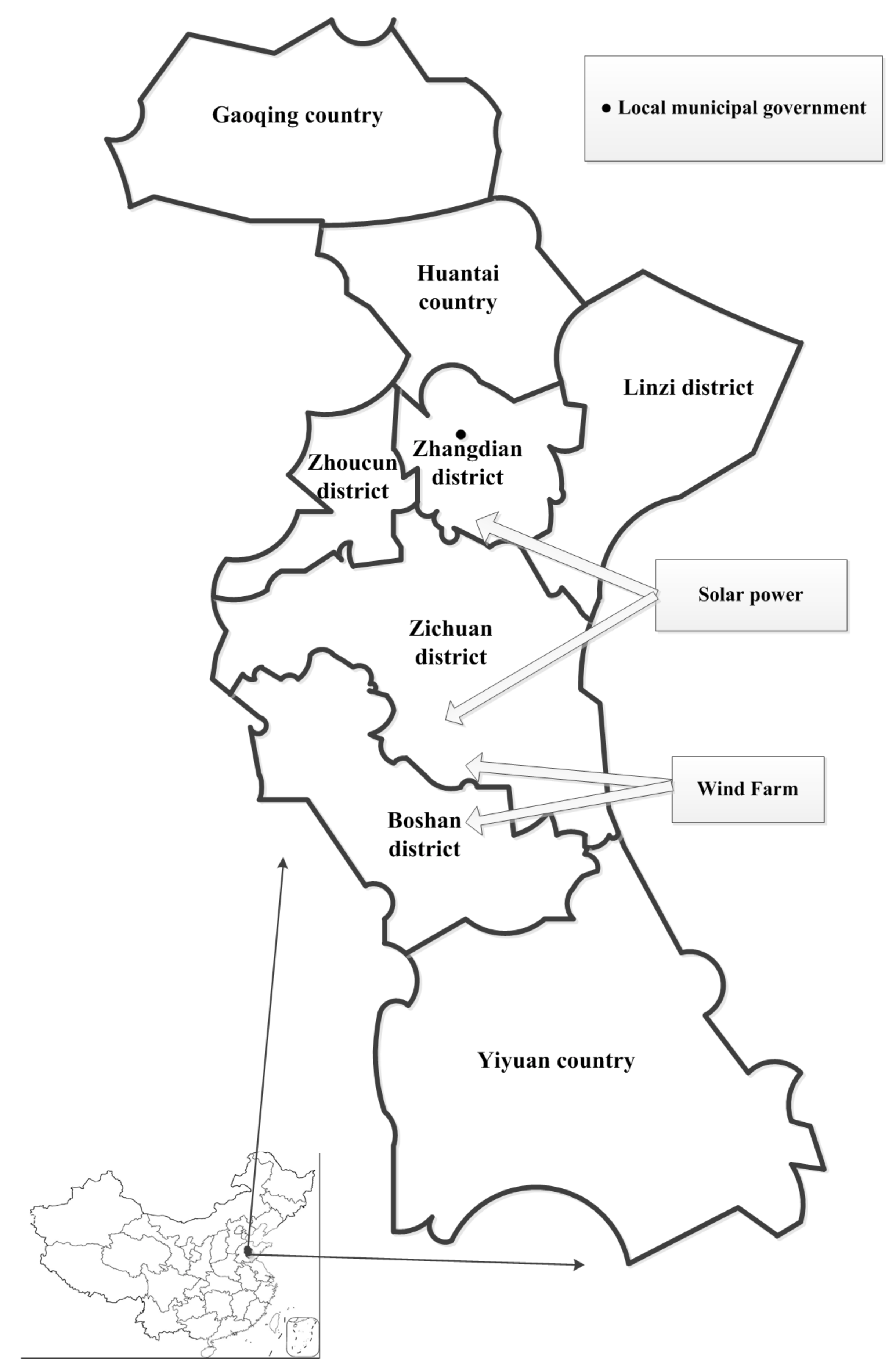
3.1. Overview of Energy System in Zibo City

Zibo City (35°55′20″~37°17′14″ N, 117°32′15″~118°31′00″ E), as shown in Figure 1, is located in the middle of Shandong province, China. Zibo City governs Zhangdian district, Zichuan district, Boshan district, Zhoucun district, Linzi district, Huantai country, Gaoqing country, and Yiyuan country, with a total area of 5938 km2 and a total population of 4.61 million in 2014 [38]. In Zibo City, the manufacturing industry plays a significant role in supporting regional economic development; especially the ceramics manufacturing industry is famous around the world. For example, in 2014, the income of ceramic industry reached 112.8 billion yuan. In addition, high-new-technology industries (e.g., new materials, fine chemicals, and biological medicines) and other traditional industries (e.g., petrochemical industry, pharmaceuticals, metallurgy, and machinery and textiles) are developing rapidly in recent years. Moreover, in 2014, gross agricultural product reached to RMB 25.22 billion yuan, and the tertiary industry increased by RMB 163.45 billion yuan compared with 2013. In general, the rapid social-economic development is closely related with a higher power consumption. According to regional energy system statistic data in recent years, local electric-power generation is far from satisfying increasing regional demands.
Generally, the main electricity generation in Zibo City mainly relies on coal-fired power. The cogeneration power plays a large proportion in all electricity generation in Zibo, which could not only meet the demand of the district heating, but also greatly improve efficiency of coal resource utilization. In order to meet environmental requirements, there would have to be total consumption control on coal resources, according to the regional development plan from Zibo Municipal Development and Reform Committee. In addition, Zibo is abundant in renewable energy resources, such as solar, biomass, and wind, that have been considered as the primary options for addressing the crisis of electric-power shortage, and air pollutant and greenhouse gas mitigation. For instance, the average annual sunshine time reaches up to 2542.6 h with a greater potential and space for solar power and heat utilization. Moreover, throughout the windy corridor, in the surrounding of Boshan District and the southern mountain areas of Zichuan District, Zibo possesses the excellent conditions to build wind farms. According to regional energy development strategy of Zibo City (2010–2020), a greater number of renewable energy development plans have been promoted for adjusting the existing electric-power system structure, including 114 MW, 50 MW, and 244.5 MW of biomass and garbage power, solar, and wind power generation capacity by 2015, respectively. As a result, it will be helpful for alleviating the contradiction between energy supply capacity and consumption demands, and reducing atmospheric pollutants and carbon emission.
Although renewable energy has achieved development, and the government has also made great efforts to change regional electric-power structure, it still faces many challenges in electric-power system management. As a result of regional economic development, urbanization advance, and population growth, electric-power consumption and environmental quality requirement would be increasingly prominent, leading to an urgent need for regional electric-power structure adjustment. In this study, an inexact regional electric-power system optimization model is developed through multistage stochastic inexact robust programming for solving the following questions: (1) how to develop electric-power generation schemes for different power conversion technologies under air pollution and carbon mitigation requirements; (2) how to plan the overall development of renewable power conversion technologies and the proportion of imported electricity; (3) how to formulate more reasonable decision alternatives for decision-makers under different trade-offs between system cost and risk.

3.2. Electric-Power System Optimization Model Formulation

The developed multistage stochastic inexact robust programming is considered for regional electric-power system management in Zibo City. The objective is to achieve the optimal plans of electric-power supply with minimized system costs. The renewable power generation development, capacity expansion, and air pollutant and carbon emission reduction were also considered. Thus, the optimized model can be developed as follows:
M i n   f ± = f 1 ± + f 2 ± + f 3 ± + f 4 ± + f 5 ± + f 6 ± f 7 ± + f 8 ±  
[Costs for energy resources consumption]
f 1 ± = p = 1 P t = 1 T P E C p t ± ( A E p t ± + p t h D E p t h ± ) E F p t ±
[Costs for power generation]
f 2 ± =   p = 1 P t = 1 T P V p t ± A E p t ± + p = 1 P t = 1 T h = 1 H p t h ( P V p t ± + P P p t ± ) D E p t h ±
[Cost for the district heating]
f 3 ± = p = 1 P t = 1 T C V p t ± ( A H p t ± + D H p t ± )
[Costs for the expansion of installed capacity]
f 4 ± = p = 1 P t = 1 T h = 1 H p t h ( Y E H p t h ± A p t ± + X E H p t h ± B p t ± )
[Costs for atmospheric pollutants treatment]
f 5 ± = i = 1 I p = 1 P t = 1 T A E p t ± ξ i p t ± ( 1 η i p t ± ) C P C i t ± + i = 1 I p = 1 P t = 1 T h = 1 H p t h D E p t h ± ξ i p t ± ( 1 η i p t ± ) D P C i t ±
[Costs for imported electric power]
f 6 ± = t = 1 T p t h I E t h ± I P E t ±
[Subsidies for renewable energy generation]
f 7 ± = p = 3 P t = 1 T ( A E p t ± + p t h D E p t h ± ) S U p t ±
[Robust function]
f 8 ± = λ p = 1 P t = 1 T h = 1 H p t h [ ε p t h ± p = 1 P h = 1 H p t h ε p t h ± + 2 θ p t h ± ]
where,
ε   p t h ± = P E C p t ± D E p t ± E F p t ± + ( P V p t ± + P P p t ± ) D E p t h ± + I E t ± I P E t ± + ( Y E H p t h ± A p t ± + X E H p t h ± B p t ± ) + i = 1 I D E p t h ± ξ i p t ± ( 1 η i p t ± ) D P C i t ± D E p t h ± S U p t ±
where f ± is the objective of the proposed model (million yuan ¥); p is the power conversion technologies, p = 1, 2, 3, 4, and 5 for combined heat and power (CHP), hydroelectric power, solar photovoltaic power, wind power, and garbage power and biomass power, respectively; i denotes different atmospheric pollutants, i  = 1, 2, 3, 4 for CO2, SO2, NOx, and particulate matter, respectively; t is the planning period; h denotes the electric-power demand level, h = 1 for low level, h = 2 for medium level, and h = 3 for high level, respectively. Z p t ± is the amount of energy resource consumption for power conversion technology p (PJ); P E C p t ± represents the energy price for technology p (million ¥/PJ); P V p t ± and P P p t ± are the variable cost for power generation and the penalty cost of excess power generation of technology p (million ¥/GWh); A E p t ± denotes the pre-regular electric-power generation by technology p (GWh); D E p t h ± is the excess power generation by technology p under different electric-power deficiency levels h (GWh); C V p t ± represents the variable cost for heat generation by technology p (million ¥/PJ); A H p t ± is the amount of district heat supply by technology p (PJ); D H p t ± denotes the amount of district heat supply by expanded capacity X E H p t h ± (PJ); A p t ± and B p t ± are the fixed-charge cost and variable cost for capacity expansion of technology p (million ¥); S U p t ± is the subsidy for new renewable energy generation p (million ¥/GW); Y E H p t h ± represents the binary variable for determining the capacity choice of technology p expansion (0 denotes no expansion; 1 represents expansion); X E H p t h ± is the capacity expansion amount for technology p under different electric-power deficiency levels h (GW); I E t h ± denotes imported power amount (GWh); I P E t ± is the cost of imported power (million ¥/GWh); C P C i t ± and D P C i t ± are the removal cost of pollutant i treatment and the penalty cost of excess pollutant i treatment for technology p (million¥/ton); ξ i p t ± is the generation rate of pollutant from technology (ton/GWh).
Constraint:
[Constraints for electric-power supply and demand balance]
p = 1 P ( A E p t ± + D E p t h ± ) + I E t h ± A D E t h ± , t , h
( A E p t ± + D E p t h ± ) S T p t ± I C p t ± , p , t , h
A E p t ± D E p t h ± 0 , p , t , h
I E t h ± 40 % A D E t h ± , t , h
[Constraints for the district heating supply and demand balance]
p = 1 P ( A H p t ± + D H p t ± ) T H t h ± , t , h
A H p t ± D H p t h ± 0 , p , t , h
[Constraint for combined heat and power generation balance]
Q ± m 1 t ± = B Q ( A E 1 t ± 1 E S ± C E ± + A H 1 t ± 1 H S ± C H ± ) t ;  
[Constraints for the heat-to-electric ratio of cogeneration plant]
A H 1 t ± + D H 1 t ± = ( A E 1 t ± + D E 1 t h ± ) κ ± , t
X E H 1 t h ± S T 1 t ± = D H 1 t ± κ ± , t
[Constraint for the total thermal efficiency of thermal power plant from national policy]
( A E 1 t ± + A H 1 t ± ) 45 % Q ± m t ± , t
[Constraints for environment capacity (CO2, PM, SO2, and NOx emission)]
p = 1 P ( A E p t ± + D E p t h ± ) ξ i p t ± ( 1 η i p t ± ) M A G E i t , i , t , h
[Constraints for installed capacity]
I C p t ± = I C P p + Y E H p t h ± X E H p t h ± C I C p t ± , t = 1 , p , h  
I C p t ± = I C p ( t 1 ) ± + Y E H p t h ± X E H p t h ± C I C p t ± , t > 1 , p , h
[Constraints for capacity expansion]
Y E H p t h ± { = 1 , if   capacity   expansion   is   undertaken = 0 , otherwise , p , t , h
0 X E H p t h ± M p t Y E H p t h ± , p , t , h
[Constraints for generation proportion of different technologies]
A E 1 t ± + D E 1 t h ± γ t ± A D E d t h ± , t , h
p = 3 5 ( A E p t ± + D E p t h ± ) δ A D E d t h ± ,   t ,   h
[Constraints for availabilities of energy resources]
( A E p t ± + D E p t h ± ) · E E p t ± Z p t ± ,   p , t , h
[Robust constraints]
ε p t h ± p = 1 P h = 1 H p t h ε p t h ± + θ p t h ± 0 , p , t , h
where A D E t h ± denotes the electricity demand under different electric-power deficiency levels h during period t (GWh); T H t h ± is the district heat demand under different deficiency levels h during period t (PJ); Q ± is the heating value of coal (PJ/ton); m 1 t ± represents the coal quantity fed to combined heat and power (CHP) (ton); B Q denotes the calorific value of coal (PJ/ton); E S ± is the electricity consumption rate of thermal power plant; C E ± is the standard coal consumption of power generation of thermal power plant (ton/PJ); H S ± represents the heat loss of the facilities; C H ± is the standard coal consumption of heat supply of thermal power plant (ton/PJ); κ ± denotes heat-to-electric ratio; γ t ± denotes the proportion of thermal power; η i p t ± is the removal efficiency of pollutant i from technology p ; ξ i p t ± denotes the emission intensity of pollutant i from technology p (103 ton/GWh); M A G E i t is the total allowable amount of pollutant i emission (103 ton); M p t ± and N p t ± are the constraints for the upper and lower capacity expansion bound of technology p (GW); S T p t ± is the operation hours of technology P in period t (h); δ denotes the percentage of power generation amount by renewable energy resources; I C P p is the initial installed capacity of power conversion technology p (GW); I C p t ± represents the total installed capacity of technology p (GW); C I C p t ± denotes the closed installed capacity of “developing large units and suppressing small ones” in period t (GW); E F p t ± is the resources conversion efficiency of technology p (PJ/GWh).
The planning horizon is considered as being from 2016 to 2021, and divided into two periods with a 3-year interval for each period. The related technical-economic information was obtained through analyzing many representative energy-related governmental reports and plans. Table 1 presents power demands and the occurrence probabilities of each demand level (25%, 55%, and 20%). According to Zibo Statistics Bureau (from 1990 to 2014), and the forecasting information of electric-power demand by the government, three electricity generation targets are selected. Table 1 also shows the district heating demands during the planning horizon. To achieve the targets of renewable power generation and emission reduction, in the electric-power system, some scenarios are designed, which corresponds to environmental constraints and renewable power development constraints (i.e., renewable energy generation in period 1 and 2 accounts for 5% and 10% of the total regional power consumption, respectively).

4. Result Analysis and Discussion

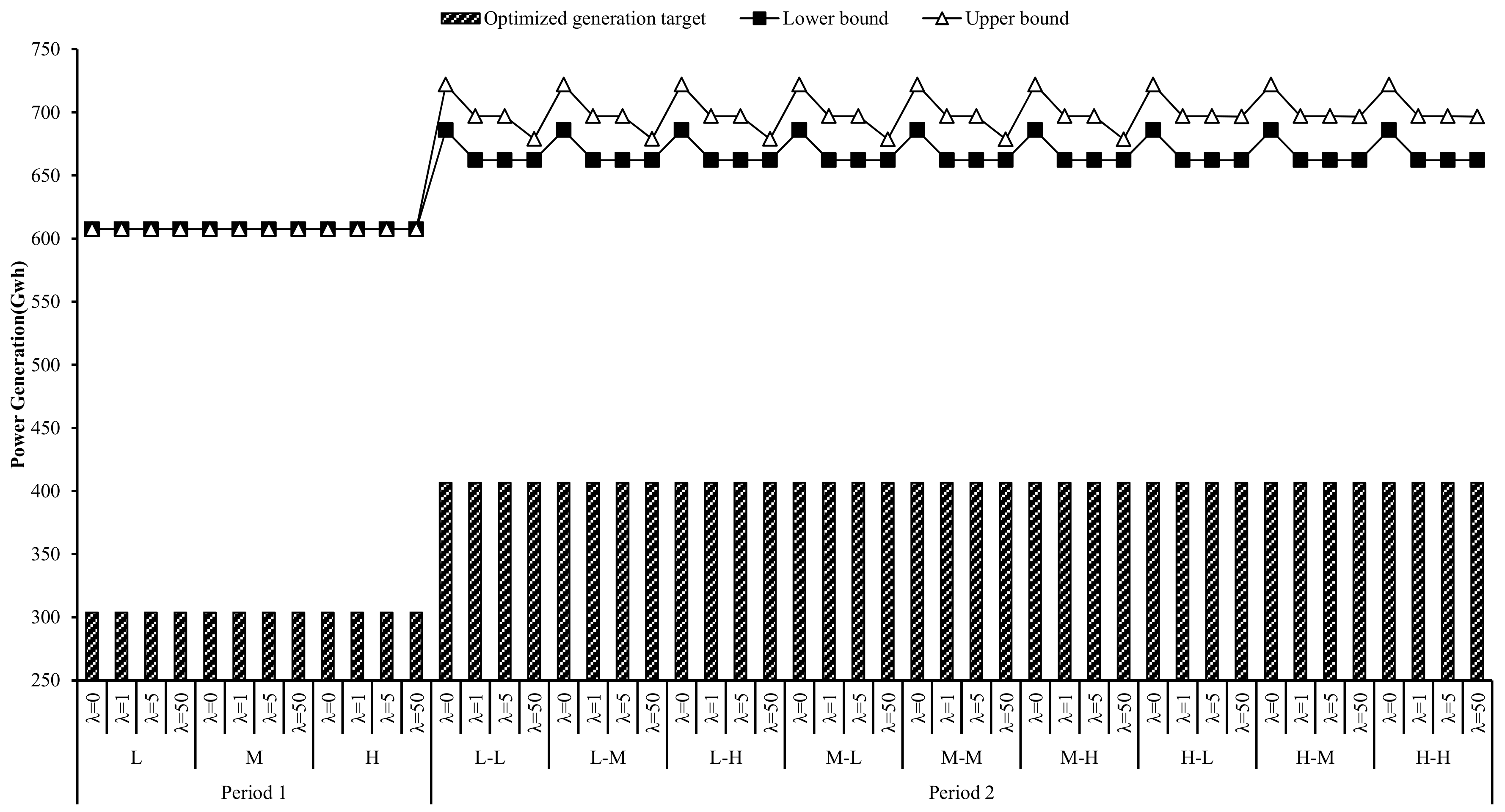
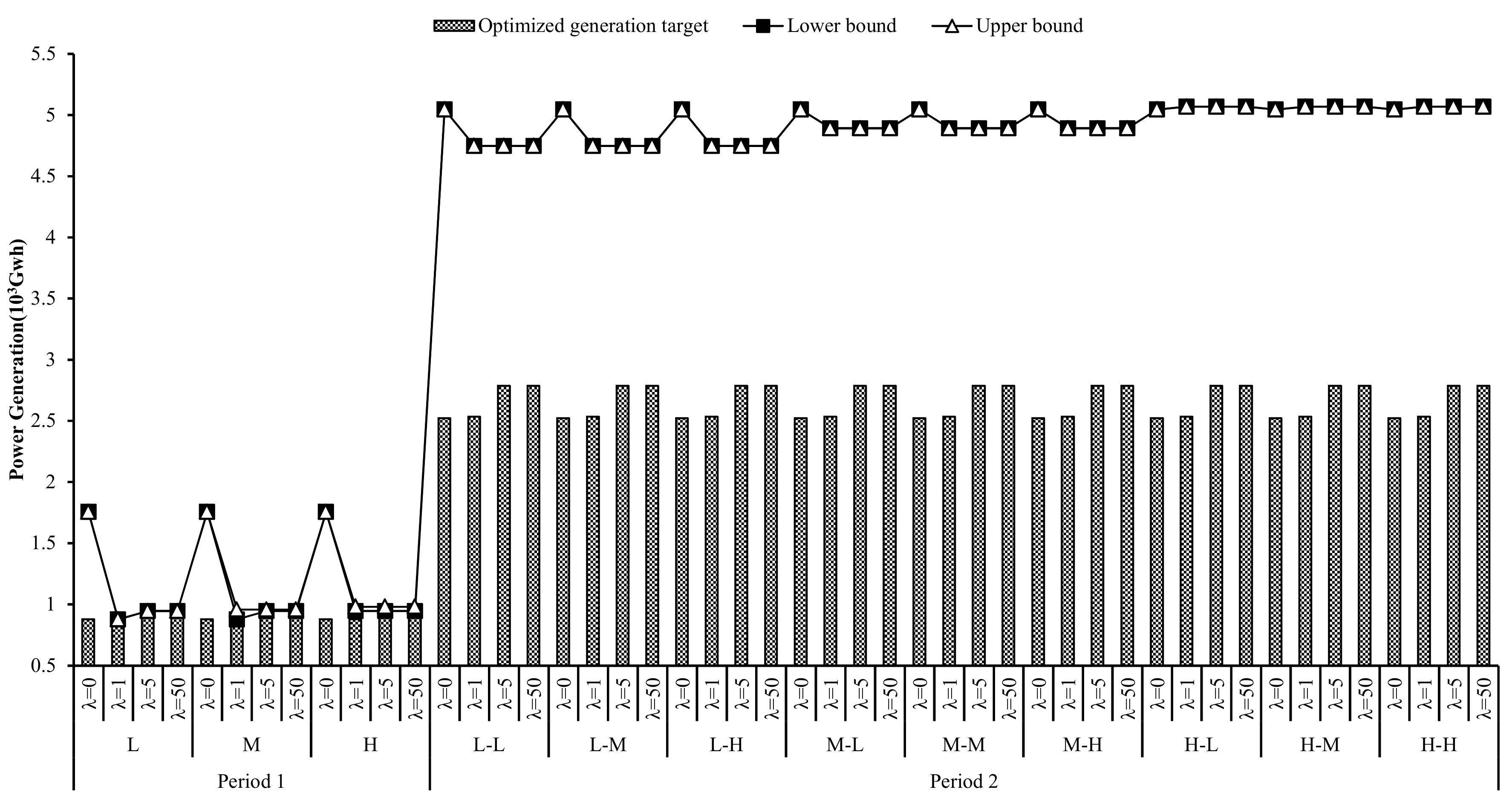
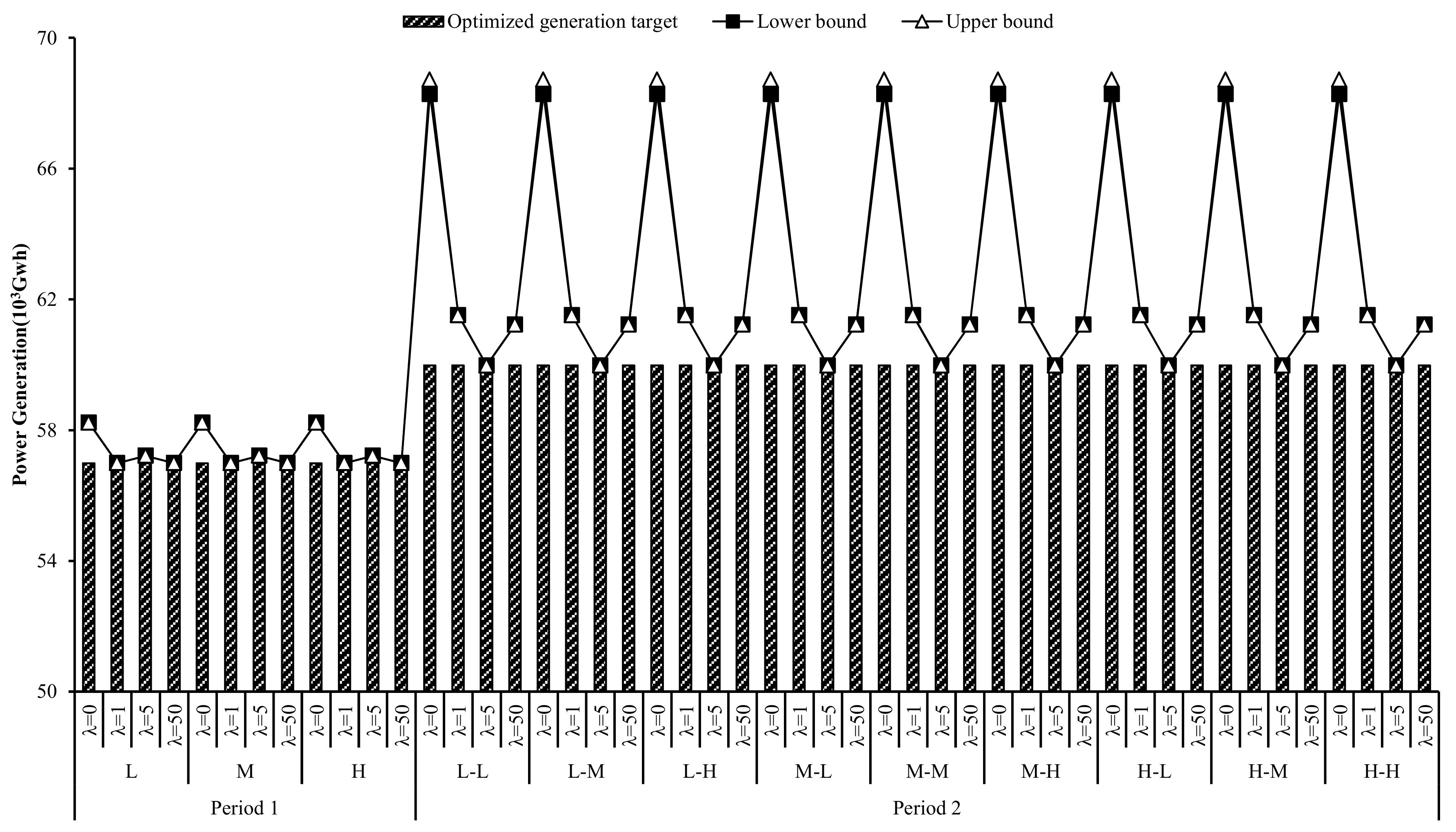
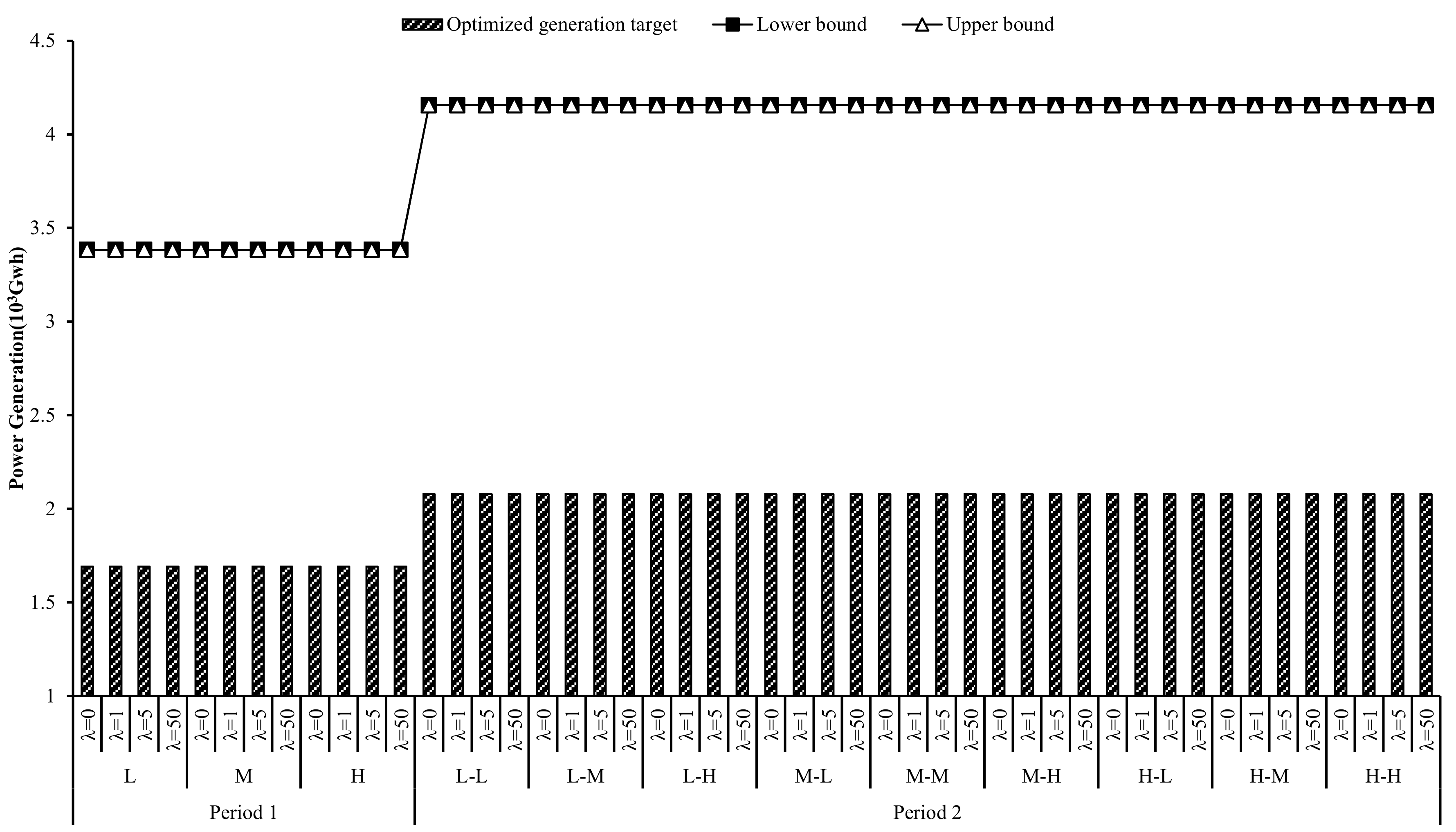
4.1. Electricity-Generation Plan

Table 2, Table 3, Table 4 and Table 5 present the optimal solutions of electric-power generation schemes of different technologies with different λ values, under different demand levels, during the whole planning horizon. The optimal combined electricity and heat generation targets in period 2 would be greater than that in period 1. In period 1, the generation amount of combined electricity and heat would be 56.99 × 10³ GWh in period 1, and 59.98 × 10³ GWh in period 2 under different λ values. Furthermore, power generation amount of CHP would increase. For example, in period 1, under medium demand level, power generation amount by CHP would be 58.23 × 10³ GWh, 56.99 × 10³ GWh, 57.22 × 10³ GWh, and 56.99 × 10³ GWh, as λ is fixed with the values of 0, 1, 5 and 50, respectively; under medium–medium level (with the probability of 30.25%) in period 2, power generation amount would be (68.28, 68.72) × 103 GWh, 61.51 × 10³ GWh, 59.98 × 10³ GWh, and 61.22 × 10³ GWh, respectively. It indicated that the CHP is a more economical and stable way for power supply with the demand of electricity increasing, and along with regional electric-power structure optimization, the combined heat and power would still be the main choice for supporting regional electric-power supply.
Among these renewable power generation technologies, clean electricity would mainly come from solar power, wind power, and biomass and garbage power (BGP). The optimized electricity generation for wind power would be 3.38 × 10³ GWh and 4.16 × 10³ GWh in periods 1 and 2, respectively. The wind power would play a significant role in renewable power development during the planning horizon. For example, in period 1, wind power generation would occupy about 3% of total electricity consumption, and 60% of total renewable power generation under different demand level; in period 2, the proportion would increase from about 3% to 4% of total electricity consumption, and be 40% of total renewable power generation. Since wind power possesses the characteristic of cleanliness and the condition of convenience in this region, wind power would be developed as a priority. In addition, BGP power generation would increase significantly during the whole planning horizon. For example, in period 1 under medium level (with the probability of 55%), power generation amount of BGP would be 1.76 × 10³ GWh, (877.53, 958.13) GWh, (945.98, 958.13) GWh, and (945.98, 958.13) GWh under λ with the values of 0, 1, 5, and 50, respectively; in period 2 under medium–medium level, power generation amount of BGP would be 5.05 × 10³ GWh, 5.07 × 10³ GWh, 5.07 × 10³ GWh, and 5.07 × 10³ GWh with λ fixed as 0, 1, 5 and 50, respectively. The proportion of biomass and garbage power generation would rise from about 1% in period 1, to 5% in period 2 of total electricity consumption, and 20% in period 1 to 50% in period 2 of total renewable power generation. In Zibo city, the hydropower would have a smaller scale under water resource and geography limitation. In general, renewable power generation amount would change as λ values vary, and the stability of the regional electric-power supply would be enhanced as the total renewable power generation amount increases.
Figure 2, Figure 3, Figure 4 and Figure 5 show the optimized solutions for electric-power generation schemes under different λ values. Electric-power generation amount of CHP would be decreased as λ increases. For example, in period 2 under medium–medium level, electric-power amount generated by CHP would be (68.28, 68.72) × 103 GWh, 61.51 × 10³ GWh, 59.98 × 10³ GWh, and 61.22 × 10³ GWh under λ fixed as 0, 1, 5, and 50, respectively. It indicated that the risk of system failure, which means higher CO2 and pollutants discharged from cogeneration exceeding the regulated limitation, would decrease as λ increases. In general, relatively lower power generation of CHP would promote emissions reduction and evade the risk of regional energy system.
As shown in Figure 3, solar power generation amount would be decreased as λ value increases. For example, in period 2 under medium–medium level, the electricity generated by solar power would be (685.87, 721.97) GWh, (662.16, 697.01) GWh, (662.16, 697.01) GWh, and (662.16, 678.65) GWh as λ is fixed with the values of 0, 1, 5, and 50, respectively. Since the regional power supply of solar power has the characteristic of instability and higher cost, the stability and security of system power supply would increase as λ increases. Electric power generated by BGP would decrease as λ increases (Figure 5). For instance, under λ fixed with the values of 0, 1, 5, and 50, power generation amount of BGP would be 1.76 × 10³ GWh, (877.53, 958.13) GWh, (945.98, 958.13) GWh, and (945.98, 958.13) GWh in period 1 under medium level, respectively; the generation amount would be 5.05 × 10³ GWh, 5.07 × 10³ GWh, 5.07 × 10³ GWh, and 5.07 × 10³ GWh under medium–medium level in period 2, respectively. A higher power generation of BGP would lead to a higher pollutants and CO2 emission, which would violate environmental constraints of the system. As λ increases, the power generation of BGP would be reduced. In summary, the total renewable power generation amount would increase as λ values increase. Thus, as λ values increases, the system failure risk would be lessened; meanwhile, the security and stability would be enhanced.

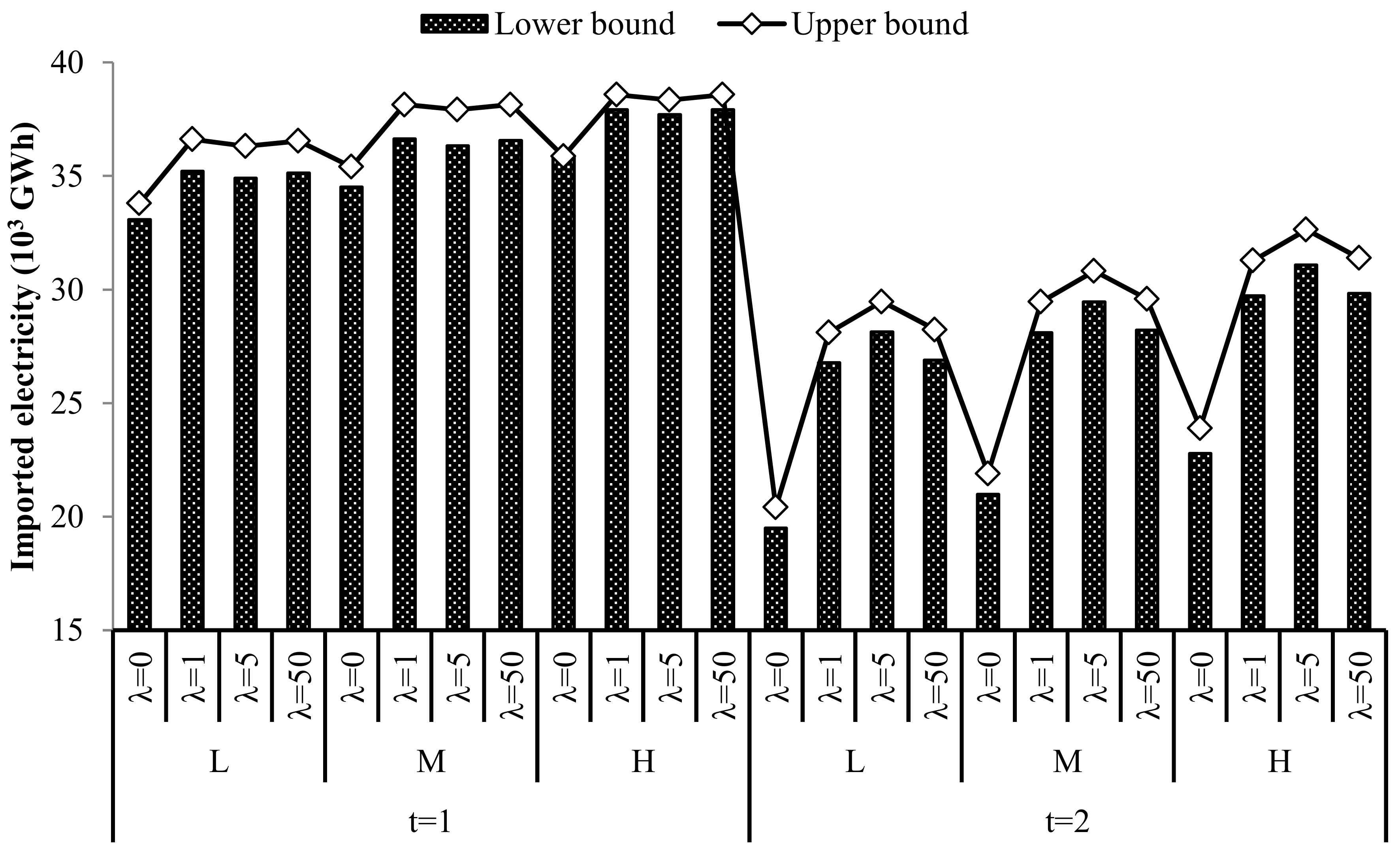
4.2. Imported Electricity Scheme

Figure 6 presents the imported electric power amount during the planning horizon. It would decrease from period 1 to 2 under different power demand levels. For example, with λ fixed as 0,1,5, and 50, the imported power amount would be (34.5, 35.41) × 103 GWh, (36.62, 38.15) × 103 GWh, (36.32, 37.92) × 103 GWh, and (36.55, 38.15) × 103 GW h under medium level in period 1, respectively; (20.98, 21.9) × 103 GWh, (28.1, 29.46) × 103 GWh, (29.46, 30.82) × 103 GWh, and (28.21, 29.59) × 103 GWh under medium–medium demand level in period 2, respectively. It indicated that the imported power amount would be decreased with regional power generation and power structure adjustment increasing, and the amount of imported electricity would rise as λ increases. For instance, under medium level in period 1, the amount would be (34.5, 35.41) × 103 GWh under λ = 0 and (36.55, 38.15) × 103 GWh under λ = 50. As a result, it would lead to a smaller system risk and enhanced system feasibility, which could also promote the energy conservation and emissions reduction to some degree.

4.3. CO2 and Air Pollution Control
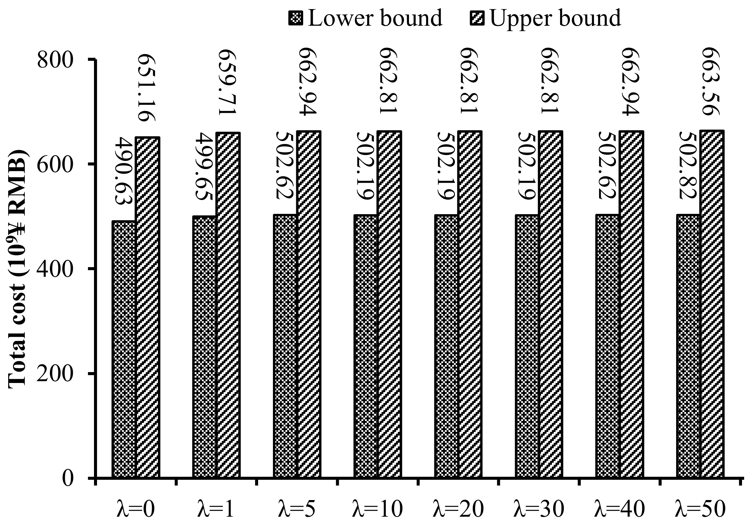
Table 6 shows the solutions of optimized air pollutants and CO2 emission. The air pollutants and CO2 emission amount would decrease. For example, under λ = 5, the amount of CO2 emissions would decrease from (60.54, 61.01) × 106 ton in period 1 to (55.6, 56.17) × 106 ton in period 2; the amount of SO2 emissions would decrease from (69.03, 80.23)× 103 ton in period 1 to (45.35, 66.78) × 103 ton in period 2; the amount of NOx emissions would be (59.27, 83.71) × 103 ton and (35.61, 70.75) × 103 ton in period 1 and 2; the amount of PM10 emissions would decrease from (9.56, 12.43) × 103 ton in period 1 to (4.89, 7.02) × 103 ton in period 2, respectively. The reasons for decreasing emission are that firstly, the technology and facilities would be updated to reduce the average emissions level; secondly, due to the power structure optimization in the first period, renewable energy has been developed to some degree, which could make contributions to energy conservation and emissions reduction. In addition, the effect of emission mitigation could be better under considering system risk aversion. It indicates that the results would lead to a lower system risk and more robust regional energy system, which is important for achieving sustainable development and better environment quality.

4.4. System Cost

Figure 7 shows the total system costs under different scenarios during the planning periods. The energy system cost in Zibo city would have a slight increase trend as λ levels increase. For instance, under the scenarios of λ with the values of 0, 1, 5, and 50, the system cost would be RMB¥ (490.63, 651.16) × 109, RMB¥ (499.65, 659.71) × 109, RMB¥ (502.62, 662.94) × 109, and RMB¥ (502.82, 663.56) × 109, respectively. As λ levels increasing, the system failure risk would be reduced, and the system cost would be increased. Conversely, a lower λ level would bring about a higher system risk and a lower system cost. It indicated that if the decision-makers aim to lower costs, a higher system risk may occur.
Based on the above analyses, these indicated that the optimized solutions are able to support regional energy system management for making integrated schemes of power generation, capacity expansion, air pollutant and CO2 emission reduction under different renewable energy development targets and environmental quality requirements. The solutions with lower and upper bounds are helpful for generating decision alternatives representing various options. Cost–risk analysis can be obtained through integrated the stochastic robust optimization method into the multistage stochastic programming in regional energy system management.

5. Conclusions

In this study, a multistage stochastic inexact robust programming was proposed for supporting regional electric-power system structure optimization and management. The model covered the district heating supply, power generation, and air pollutant mitigation coupled with relevant technique constraints and governmental policies. Comparing the solutions optimized by the model with the strategies carried out in the real world, the former emerged with obvious advantages, which can lead to a more prosperous future. In addition, the developed method could be valuable for obtaining trade-off schemes between system economy and risks that are introduced by system’s uncertainties according to decision-makers’ willingness. An energy system structure management of Zibo City, China, is used as a case study for verifying the efficiency of the developed model. Optimized schemes of power generation, capacity expansion, air pollutant and CO2 emission reduction, and system cost were analyzed. The results indicated that under different requirements of renewable energy development, and pollutant and CO2 mitigation, traditional power generation technology would still be increased, attributing to its lower costs and traditional energy resources structure based on the thermal power generation. In addition, renewable energy would also play an important role in solving energy, resource, and environmental pressures; renewable power generation amount would be rising continuously, though it might develop slowly for a certain period of time.
However, a number of limitations also exist in the proposed model of this study. Firstly, in the optimization model, many energy industrial processes are not considered, and only generation processes and energy-related environmental problems are involved in this study. In order to obtain more comprehensive management schemes, more energy development and utilization patterns could be considered. Second, compared with other optimization methods, the model would be infeasible in addressing the high uncertainties in the model parameters; and through introducing different λ values in the model, regional energy-managers cannot directly obtain suitable management schemes. Therefore, further research can strengthen knowledge and mitigate these limitations in the future.

Author Contributions

Y.X., L.W. and L.J. designed the manuscript and developed the models; Y.X. drafted the manuscript; L.W. and D.X. collected the data and revised the manuscript; G.H., Y.X. and D.X. checked the content and revised the manuscript. All authors made contributions to the study and the writing of the manuscript.

Funding

The National Natural Science Foundation of China (51609003 and 71603016), the China Postdoctoral Science Foundation funded project (Grand No.2015M580046 and Grand No.2015M580034), and the Fundamental Research Funds for the Central Universities (FRF-BD-18-015A).

Acknowledgments

This research was supported by the National Natural Science Foundation of China (51609003 and 71603016), the China Postdoctoral Science Foundation funded project (Grand No.2015M580046 and Grand No.2015M580034), and the Fundamental Research Funds for the Central Universities (FRF-BD-18-015A). The authors are grateful to the anonymous reviewers and editors for their valuable comments and suggestions.

Conflicts of Interest

The authors declare that there are no conflicts of interest regarding the publication of this article.

References

  1. Cristóbal, J.; Guillén-Gosálbez, G.; Jiménez, L. Multi-objective optimization of coal-fired electricity production with CO2 capture. Appl. Energy 2012, 98, 266–272. [Google Scholar] [CrossRef]
  2. Dubreuil, A.; Assoumou, E.; Bouckaert, S.; Selosse, S.; MaZi, N. Water modelling in an energy optimization framework—The water-scarce middle east context. Appl. Energy 2013, 101, 268–279. [Google Scholar] [CrossRef]
  3. Cheng, G.H.; Huang, G.H.; Dong, C.; Baetz, B.W.; Li, Y.P. Interval recourse linear programming for resources and environmental systems management under uncertainty. J. Environ. Inform. 2017, 30, 119–136. [Google Scholar] [CrossRef]
  4. Luhandjulaa, M.K. Fuzzy stochastic linear programming: Survey and future research directions. Eur. J. Oper. Res. 2006, 174, 1353–1367. [Google Scholar] [CrossRef]
  5. Mackay, R.M.; Probert, S.D. Energy and environmental policies of the developed and developing countries within the evolving Oceania and South-East Asia trading bloc. Appl. Energy 1995, 51, 369–400. [Google Scholar] [CrossRef]
  6. Price, T.J.; Probert, S.D. Taiwan’s energy and environmental policies: Past, present and future. Appl. Energy 1995, 50, 41–68. [Google Scholar] [CrossRef]
  7. Shimazaki, Y.; Akisawa, A.; Kashiwagi, T. A model analysis of clean development mechanisms to reduce both CO2 and SO2 emissions between Japan and China. Appl. Energy 2011, 66, 311–324. [Google Scholar] [CrossRef]
  8. Chaaban, F.B.; Mezher, T.; Ouwayjan, M. Options for emissions reduction from power plants: An economic evaluation. Int. J. Electr. Power Energy Syst. 2004, 26, 57–63. [Google Scholar] [CrossRef]
  9. Jebaraj, S.; Iniyan, S. A review of energy models. Renew. Sustain. Energy Rev. 2006, 10, 281–311. [Google Scholar] [CrossRef]
  10. Cai, Y.P.; Tan, Q.; Huang, G.H.; Yang, Z.F.; Lin, Q.G. Community-scale renewable energy systems planning under uncertainty—An interval chance-constrained programming approach. Renew. Sustain. Energy Rev. 2009, 13, 721–735. [Google Scholar] [CrossRef]
  11. Dincer, I.; Rosen, M.A. Exergy, energy, environment and sustainable development. Appl. Energy 2014, 64, 427–440. [Google Scholar] [CrossRef]
  12. Mukherjee, U.; Maroufmashat, A.; Narayan, A.; Elkamel, A.; Fowler, M. A stochastic programming approach for the planning and operation of a power to gas energy hub with multiple energy recovery pathways. Energies 2017, 10, 868. [Google Scholar] [CrossRef]
  13. Li, W.; Bao, Z.; Huang, G.H.; Xie, Y.L. An inexact credibility chance-constrained integer programming for greenhouse gas mitigation management in regional electric power system under uncertainty. J. Environ. Inform. 2018, 31, 111–122. [Google Scholar] [CrossRef]
  14. Tang, Z.C.; Xia, Y.J.; Xue, Q.; Liu, J. A non-probabilistic solution for uncertainty and sensitivity analysis on techno-economic assessments of biodiesel production with interval uncertainties. Energies 2018, 11, 588. [Google Scholar] [CrossRef]
  15. Cai, Y.P.; Huang, G.H.; Lu, H.W.; Yang, Z.F.; Tan, Q. I-VFRP: An interval-valued fuzzy robust programming approach for municipal waste-management planning under uncertainty. Eng. Optim. 2009, 41, 399–418. [Google Scholar] [CrossRef]
  16. Li, Y.F.; Li, Y.P.; Huang, G.H.; Chen, X. Energy and environmental systems planning under uncertainty—An inexact fuzzy-stochastic programming approach. Appl. Energy 2010, 87, 3189–3211. [Google Scholar] [CrossRef]
  17. Li, Y.P.; Huang, G.H.; Chen, X. Planning regional energy system in association with greenhouse gas mitigation under uncertainty. Appl. Energy 2011, 88, 599–611. [Google Scholar] [CrossRef]
  18. Huang, C.Z.; Nie, S.; Guo, L.; Fan, Y.R. Inexact fuzzy stochastic chance constraint programming for emergency evacuation in Qinshan nuclear power plant under uncertainty. J. Environ. Inform. 2017, 30, 63–78. [Google Scholar] [CrossRef]
  19. Sheikhahmadi, P.; Mafakheri, R.; Bahramara, S.; Damavandi, M.Y.; Catalão, J.P.S. Risk-based two-stage stochastic optimization problem of micro-grid operation with renewable and incentive-based demand response programs. Energies 2018, 11, 610. [Google Scholar] [CrossRef]
  20. Li, Y.P.; Huang, G.H.; Nie, S.L. An interval-parameter multi-stage stochastic programming model for water resources management under uncertainty. Adv. Water Resour. 2006, 29, 776–789. [Google Scholar] [CrossRef]
  21. Li, G.C.; Huang, G.H.; Lin, Q.G.; Chen, Y.M.; Zhang, X.D. Development of an interval multi-stage stochastic programming model for regional energy systems planning and GHG emission control under uncertainty. Int. J. Energy Res. 2012, 36, 1161–1174. [Google Scholar] [CrossRef]
  22. Hu, Q.; Huang, G.H.; Cai, Y.P.; Xu, Y. Energy and environmental systems planning with recourse: Inexact stochastic programming model containing fuzzy boundary intervals in objectives and constraints. J. Energy Eng. 2013, 139, 169–189. [Google Scholar] [CrossRef]
  23. Xie, Y.L.; Li, Y.P.; Huang, G.H.; Li, Y.F. An interval fixed-mix stochastic programming method for greenhouse gas mitigation in energy systems under uncertainty. Energy 2010, 35, 4627–4644. [Google Scholar] [CrossRef]
  24. Wu, C.B.; Huang, G.H.; Li, W.; Xie, Y.L.; Xu, Y. Multistage stochastic inexact chance-constraint programming for an integrated biomass-municipal solid waste power supply management under uncertainty. Renew. Sustain. Energy Rev. 2015, 41, 1244–1254. [Google Scholar] [CrossRef]
  25. Golari, M.; Fan, N.; Jin, T.D. Multistage stochastic optimization for production-inventory planning with intermittent renewable energy. Prod. Oper. Manag. 2016, 26, 409–425. [Google Scholar] [CrossRef]
  26. Fu, Z.H.; Wang, H.; Lu, W.T.; Guo, H.C.; Li, W. An inexact multistage fuzzy-stochastic programming for regional electric power system management constrained by environmental quality. Environ. Sci. Pollut. 2017, 24, 28006–28016. [Google Scholar] [CrossRef] [PubMed]
  27. Wang, L.; Huang, G.H.; Wang, X.Q.; Zhu, H. Risk-based electric power system planning for climate change mitigation through multi-stage joint-probabilistic left-hand-side chance-constrained fractional programming: A Canadian case study. Renew. Sustain. Energy Rev. 2018, 82, 1056–1067. [Google Scholar] [CrossRef]
  28. Fan, Y.; Huang, G.H.; Huang, K.; Baetz, B.W. Planning water resources allocation under multiple uncertainties through a generalized fuzzy two-stage stochastic programming method. IEEE. Trans. Fuzzy Syst. 2015, 23, 1488–1504. [Google Scholar] [CrossRef]
  29. Aseeri, A.; Bagajewicz, M.J. New measures and procedures to manage financial risk with applications to the planning of gas commercialization in Asia. Comput. Chem. Eng. 2004, 28, 2791–2821. [Google Scholar] [CrossRef]
  30. Ruszczyński, A.; Shapiro, A. Optimization of risk measures. Risk Insur. 2004, 10, 119–157. [Google Scholar]
  31. Chen, C.; Li, Y.P.; Huang, G.H. An inexact robust optimization method for supporting carbon dioxide emissions management in regional electric-power systems. Energy Econ. 2013, 40, 441–456. [Google Scholar] [CrossRef]
  32. Xie, Y.L.; Huang, G.H.; Li, W.; Ji, L. Carbon and air pollutants constrained energy planning for clean power generation with a robust optimization model—A case study of Jining City, China. Appl. Energy 2014, 136, 150–167. [Google Scholar] [CrossRef]
  33. Huang, G.H.; Baetz, B.W.; Patry, G.G. A grey linear programming approach for municipal solid waste management planning under uncertainty. Civ. Eng. Syst. 1992, 9, 319–335. [Google Scholar] [CrossRef]
  34. Huang, G.H. IPWM: An interval parameter water quality management model. Eng. Optim. 1996, 26, 79–103. [Google Scholar] [CrossRef]
  35. Yu, C.S.; Li, H.L. A robust optimization model for stochastic logistic problems. Int. J. Prod. Econ. 2000, 64, 385–397. [Google Scholar] [CrossRef]
  36. Leung, S.C.H.; Tsang, S.O.S.; Ng, W.L.; Wu, Y. A robust optimization model for multi-site production planning problem in an uncertain environment. Eur. J. Oper. Res. 2007, 181, 224–238. [Google Scholar] [CrossRef]
  37. Huang, G.H.; Loucks, D.P. An inexact two-stage stochastic programming model for water resources management under uncertainty. Civ. Eng. Environ. Syst. 2000, 17, 95–118. [Google Scholar] [CrossRef]
  38. Zibo City Bureau of Statistics. Zibo City Statistical Yearbook 2014; China Statistical Press: Beijing, China, 2015.
Figure 1. Location of the study area and regional energy resources distribution.
Energies 11 02108 g001
Figure 2. The optimized cogeneration operation schemes during the planning horizon.
Energies 11 02108 g002
Figure 3. The optimized solar power generation amount in planning periods.
Energies 11 02108 g003
Figure 4. The optimized wind power generation during the whole planning horizon.
Energies 11 02108 g004
Figure 5. Optimized biomass power generation amount in the planning periods.
Energies 11 02108 g005
Figure 6. The imported electricity amount under different λ values.
Energies 11 02108 g006
Figure 7. Net system cost under different scenarios.
Energies 11 02108 g007
Table 1. Regional electricity and heat demand during the planning period.
Energy DemandDemand LevelProbability (%)T = 1T = 2
Electricity demand (103 GWh)Low20[97.11, 98.53][97.73, 99.11]
Medium60[98.53, 100.14][99.21, 100.60]
High20[99.90, 100.60][101.00, 102.60]
District heat quantity (PJ)Low20[253.59, 259.59][255.00, 263.00]
Medium60[278.68, 288.68][285.00, 293.00]
High20[288.87, 297.87][295.00, 302.00]
Table 2. The optimized power generation schemes under λ = 0.
TechnologyLevelProbability (%)Optimized Generation Target (GWh)Optimized Shortage Quantity (GWh)Optimized Generation Quantity (GWh)
CHPL2556,989.231240.1258,229.35
M5556,989.231240.1258,229.35
H2056,989.231240.1258,229.35
L-L6.2559,978.03[8302.54, 8737.05][68,280.57, 68,715.08]
L-M13.7559,978.03[8302.54, 8737.05][68,280.57, 68,715.08]
L-H559,978.03[8302.54, 8737.05][68,280.57, 68,715.08]
M-L13.7559,978.03[8302.54, 8737.05][68,280.57, 68,715.08]
M-M30.2559,978.03[8302.54, 8737.05][68,280.57, 68,715.08]
M-H1159,978.03[8302.54, 8737.05][68,280.57, 68,715.08]
H-L559,978.03[8302.54, 8737.05][68,280.57, 68,715.08]
H-M1159,978.03[8302.54, 8737.05][68,280.57, 68,715.08]
H-H459,978.03[8302.54, 8737.05][68,280.57, 68,715.08]
HydropowerL2529.0129.0158.02
M5529.0129.0158.02
H2029.0129.0158.02
L-L6.2530.8530.8561.70
L-M13.7530.8530.8561.70
L-H530.8530.8561.70
M-L13.7530.8530.8561.70
M-M30.2530.8530.8561.70
M-H1130.8530.8561.70
H-L530.8530.8561.70
H-M1130.8530.8561.70
H-H430.8530.8561.70
Solar powerL25303.74303.74607.48
M55303.74303.74607.48
H20303.74303.74607.48
L-L6.25406.53[279.34, 315.44][685.87, 721.97]
L-M13.75406.53[279.34, 315.44][685.87, 721.97]
L-H5406.53[279.34, 315.44][685.87, 721.97]
M-L13.75406.53[279.34, 315.44][685.87, 721.97]
M-M30.25406.53[279.34, 315.44][685.87, 721.97]
M-H11406.53[279.34, 315.44][685.87, 721.97]
H-L5406.53[279.34, 315.44][685.87, 721.97]
H-M11406.53[279.34, 315.44][685.87, 721.97]
H-H4406.53[279.34, 315.44][685.87, 721.97]
Wind powerL251691.761691.763383.52
M551691.761691.763383.52
H201691.761691.763383.52
L-L6.252077.832077.834155.66
L-M13.752077.832077.834155.66
L-H52077.832077.834155.66
M-L13.752077.832077.834155.66
M-M30.252077.832077.834155.66
M-H112077.832077.834155.66
H-L52077.832077.834155.66
H-M112077.832077.834155.66
H-H42077.832077.834155.66
Biomass and garbage powerL25877.53877.531755.06
M55877.53877.531755.06
H20877.53877.531755.06
L-L6.252522.632522.635045.26
L-M13.752522.632522.635045.26
L-H52522.632522.635045.26
M-L13.752522.632522.635045.26
M-M30.252522.632522.635045.26
M-H112522.632522.635045.26
H-L52522.632522.635045.26
H-M112522.632522.635045.26
H-H42522.632522.635045.26
Table 3. The optimized power generation schemes under λ = 1.
TechnologyLevelProbability (%)Optimized Generation Target (GWh)Optimized Shortage Quantity (GWh)Optimized Generation Quantity (GWh)
CHPL2556,989.23056,989.23
M5556,989.23056,989.23
H2056,989.23056,989.23
L-L6.2559,978.031536.7561,514.78
L-M13.7559,978.031536.7561,514.78
L-H559,978.031536.7561,514.78
M-L13.7559,978.031536.7561,514.78
M-M30.2559,978.031536.7561,514.78
M-H1159,978.031536.7561,514.78
H-L559,978.031536.7561,514.78
H-M1159,978.031536.7561,514.78
H-H459,978.031536.7561,514.78
HydropowerL2529.0129.0158.02
M5529.0129.0158.02
H2029.0129.0158.02
L-L6.2530.8530.8561.70
L-M13.7530.8530.8561.70
L-H530.8530.8561.70
M-L13.7530.8530.8561.70
M-M30.2530.8530.8561.70
M-H1130.8530.8561.70
H-L530.8530.8561.70
H-M1130.8530.8561.70
H-H430.8530.8561.70
Solar powerL25303.74303.74607.48
M55303.74303.74607.48
H20303.74303.74607.48
L-L6.25406.53[255.63, 290.48][662.16, 697.01]
L-M13.75406.53[255.63, 290.48][662.16, 697.01]
L-H5406.53[255.63, 290.48][662.16, 697.01]
M-L13.75406.53[255.63, 290.48][662.16, 697.01]
M-M30.25406.53[255.63, 290.48][662.16, 697.01]
M-H11406.53[255.63, 290.48][662.16, 697.01]
H-L5406.53[255.63, 290.48][662.16, 697.01]
H-M11406.53[255.63, 290.48][662.16, 697.01]
H-H4406.53[255.63, 290.48][662.16, 697.01]
Wind powerL251691.761691.763383.52
M551691.761691.763383.52
H201691.761691.763383.52
L-L6.252077.832077.834155.66
L-M13.752077.832077.834155.66
L-H52077.832077.834155.66
M-L13.752077.832077.834155.66
M-M30.252077.832077.834155.66
M-H112077.832077.834155.66
H-L52077.832077.834155.66
H-M112077.832077.834155.66
H-H42077.832077.834155.66
Biomass and garbage powerL25877.530877.53
M55877.53[0, 80.6][877.53, 958.13]
H20877.53[68.45, 103.45][945.98, 980.98]
L-L6.252534.492212.794747.28
L-M13.752534.492212.794747.28
L-H52534.492212.794747.28
M-L13.752534.492357.884892.37
M-M30.252534.492357.884892.37
M-H112534.492357.884892.37
H-L52534.492534.495068.98
H-M112534.492534.495068.98
H-H42534.492534.495068.98
Table 4. The optimized power generation schemes under λ = 5.
TechnologyLevelProbability (%)Optimized Generation Target (GWh)Optimized Shortage Quantity (GWh)Optimized Generation Quantity (GWh)
CHPL2556,989.23226.4757,215.70
M5556,989.23226.4757,215.70
H2056,989.23226.4757,215.70
L-L6.2559,978.03059,978.03
L-M13.7559,978.03059,978.03
L-H559,978.03059,978.03
M-L13.7559,978.03059,978.03
M-M30.2559,978.03059,978.03
M-H1159,978.03059,978.03
H-L559,978.03059,978.03
H-M1159,978.03059,978.03
H-H459,978.03059,978.03
HydropowerL2529.0129.0158.02
M5529.0129.0158.02
H2029.0129.0158.02
L-L6.2530.8530.8561.70
L-M13.7530.8530.8561.70
L-H530.8530.8561.70
M-L13.7530.8530.8561.70
M-M30.2530.8530.8561.70
M-H1130.8530.8561.70
H-L530.8530.8561.70
H-M1130.8530.8561.70
H-H430.8530.8561.70
Solar powerL25303.74303.74607.48
M55303.74303.74607.48
H20303.74303.74607.48
L-L6.25406.53[255.63, 290.48][662.16, 697.01]
L-M13.75406.53[255.63, 290.48][662.16, 697.01]
L-H5406.53[255.63, 290.48][662.16, 697.01]
M-L13.75406.53[255.63, 290.48][662.16, 697.01]
M-M30.25406.53[255.63, 290.48][662.16, 697.01]
M-H11406.53[255.63, 290.48][662.16, 697.01]
H-L5406.53[255.63, 290.48][662.16, 697.01]
H-M11406.53[255.63, 290.48][662.16, 697.01]
H-H4406.53[255.63, 290.48][662.16, 697.01]
Wind powerL251691.761691.763383.52
M551691.761691.763383.52
H201691.761691.763383.52
L-L6.252077.832077.834155.66
L-M13.752077.832077.834155.66
L-H52077.832077.834155.66
M-L13.752077.832077.834155.66
M-M30.252077.832077.834155.66
M-H112077.832077.834155.66
H-L52077.832077.834155.66
H-M112077.832077.834155.66
H-H42077.832077.834155.66
Biomass and garbage powerL25945.980945.98
M55945.98[0, 12.15][945.98, 958.13]
H20945.98[0, 35][945.98, 980.98]
L-L6.252787.651959.624747.27
L-M13.752787.651959.624747.27
L-H52787.651959.624747.27
M-L13.752787.652104.724892.37
M-M30.252787.652104.724892.37
M-H112787.652104.724892.37
H-L52787.652281.335068.98
H-M112787.652281.335068.98
H-H42787.652281.335068.98
Table 5. The optimized power generation schemes under λ = 50.
TechnologyLevelProbability (%)Optimized Generation Target (GWh)Optimized Shortage Quantity (GWh)Optimized Generation Quantity (GWh)
CHPL2556,989.23056,989.23
M5556,989.23056,989.23
H2056,989.23056,989.23
L-L6.2559,978.031244.5461,222.57
L-M13.7559,978.031244.5461,222.57
L-H559,978.031244.5461,222.57
M-L13.7559,978.031244.5461,222.57
M-M30.2559,978.031244.5461,222.57
M-H1159,978.031244.5461,222.57
H-L559,978.031244.5461,222.57
H-M1159,978.031244.5461,222.57
H-H459,978.031244.5461,222.57
HydropowerL2529.0129.0158.02
M5529.0129.0158.02
H2029.0129.0158.02
L-L6.2530.8530.8561.70
L-M13.7530.8530.8561.70
L-H530.8530.8561.70
M-L13.7530.8530.8561.70
M-M30.2530.8530.8561.70
M-H1130.8530.8561.70
H-L530.8530.8561.70
H-M1130.8530.8561.70
H-H430.8530.8561.70
Solar powerL25303.74303.74607.48
M55303.74303.74607.48
H20303.74303.74607.48
L-L6.25406.53[255.63, 272.34][662.16, 678.87]
L-M13.75406.53[255.63, 272.34][662.16, 678.87]
L-H5406.53[255.63, 272.34][662.16, 678.87]
M-L13.75406.53[255.63, 272.12][662.16, 678.65]
M-M30.25406.53[255.63, 272.12][662.16, 678.65]
M-H11406.53[255.63, 272.12][662.16, 678.65]
H-L5406.53[255.63, 290.11][662.16, 696.64]
H-M11406.53[255.63, 290.11][662.16, 696.64]
H-H4406.53[255.63, 290.11][662.16, 696.64]
Wind powerL251691.761691.763383.52
M551691.761691.763383.52
H201691.761691.763383.52
L-L6.252077.832077.834155.66
L-M13.752077.832077.834155.66
L-H52077.832077.834155.66
M-L13.752077.832077.834155.66
M-M30.252077.832077.834155.66
M-H112077.832077.834155.66
H-L52077.832077.834155.66
H-M112077.832077.834155.66
H-H42077.832077.834155.66
Biomass and garbage powerL25945.980945.98
M55945.98[0, 12.15][945.978, 958.13]
H20945.98[0, 35][945.978, 980.98]
L-L6.252787.651959.624747.27
L-M13.752787.651959.624747.27
L-H52787.651959.624747.27
M-L13.752787.652104.724892.37
M-M30.252787.652104.724892.37
M-H112787.652104.724892.37
H-L52787.652281.335068.98
H-M112787.652281.335068.98
H-H42787.652281.335068.98
Table 6. The amount of CO2 and air pollution emissions under different λ values.
Gaseous Emission λ LevelT = 1T = 2
CO2 (106 ton)λ= 0[61.88, 63.11][63.07, 64.10]
λ = 1[60.3, 60.77][56.82, 57.40]
Λ = 5[60.54, 61.01][55.60, 56.17]
λ = 50[60.31, 60.77][56.72, 57.30]
SO2 (103 ton)λ = 0[70.35, 82.75][51.58, 76.43]
λ = 1[68.76, 79.91][46.37, 68.28]
λ = 5[69.03, 80.23][45.35, 66.78]
λ = 50[68.76, 79.91][46.28, 68.16]
NOx (103 ton)λ = 0[60.36, 86.29][40.51, 81.00]
λ = 1[59.04, 83.38][36.41, 72.34]
λ = 5[59.27, 83.71][35.61, 70.75]
λ = 50[59.03, 83.38][36.35, 72.21]
PM (103 ton)λ = 0[9.74, 12.82][5.57, 8.04]
λ = 1[9.53, 12.38][5.00, 7.18]
λ = 5[9.56, 12.43][4.89, 7.02]
λ = 50[9.52, 12.38][5.00, 7.17]

