A Novel Protection and Location Scheme for Pole-to-Pole Fault in MMC-MVDC Distribution Grid

Abstract

Nowadays, the efficient and reliable protection and location schemes for MMC-MVDC (Modular Multilevel Converter-Medium Voltage Direct Current) grid are few. This paper is the first to propose a scheme to not only protect the feeders and the busbar, but locate the segments in MMC-MVDC grid. To improve the reliability, this paper analyzes the transient characteristics of the pole-to-pole fault and then obtains the characteristic frequency band. Based on S-transform, STCFB (S-transform characteristic frequency band) Phase of fault component is utilized to construct the identification criterion for faulty feeder and faulty segment. The whole scheme can be divided into three steps, namely, protection starting criterion, faulty feeder and busbar protection criterion, and faulty segment location criterion. Firstly, the current gradient method is utilized to quickly detect the fault and start the protection device. Secondly, the non-unit protection criterion on busbar and feeders is proposed according to STCFB Phase of the voltage and current fault component. Thirdly, according to the STCFB Phase on both sides of the feeder segment, the faulty segment can be located. A radial MMC-MVDC distribution network model was built in PSCAD/EMTDC software to evaluate the performance of the protection and location method. Simulation results for different cases demonstrate that the proposed scheme has high accuracy, good adaptability and reliability.

1. Introduction

With the development of modern power electronics technology and the increase of new energy power generation systems, the Medium Voltage Direct Current (MVDC) distribution grid will have a good prospect [1,2,3,4]. A Modular Multilevel Converter (MMC) usually has a large number of sub-modules [5]. To improve the quality of converter output waveform, nearest level modulation (NLM) method has been widely adopted [6]. Compared with two-level and three-level voltage source converters (VSCs), MMC has higher reliability and lower switching frequency [7,8]. Thus, MMC-MVDC has been favored in flexible DC projects such as ±10 kV hand-in-hand China Southern Power Grid [9].

As one of the key technologies of flexible DC distribution grid, the protection schemes of MMC-MVDC are still not mature [10]. Due to the huge differences of operation modes and fault characteristics, the protection methods of the AC system cannot be directly implemented to the MMC-MVDC distribution grid [11]. On the other hand, due to the relatively small values of resistance and inductance in DC cables, the rise rate of fault current is very high and DC circuit breakers are yet to be commercially available [12]. In order to prevent the Insulated Gate Bipolar Transistors (IGBTs) of MMC from losing controllability [13], the protection system should fast identify and isolate the faulty lines.

Traveling wave (TW)-based protection schemes satisfy the high-speed requirements in detecting and locating the faults in High Voltage Direct Current (HVDC) grid [14,15,16], but they are vulnerable to the fault resistances. Moreover, TW-based schemes need a relatively high sampling rate in distribution grid. Fault detection method using overcurrent have been proposed [17,18], but it is difficult to discriminate the faulty area and the adjacent normal areas. In addition, these methods require data synchronization. Distance protection based on the fault equivalent circuit and Kirchhoff law has been proposed for fault detection and location [19], however the calculation error and uncertainty of the transition resistance will have an impact on the calculation result due to the short length of the feeder.

The handshaking method proposed in Reference [20] identifies and isolates fault by comparing the initial current change, the current rise time interval and the current oscillation pattern at different switch locations. Nevertheless, this algorithm is a bit slow and will lead to prolonged shut down of the complete system. As multi-level segments in MMC-MVDC have no clear boundaries between each other, the schemes based on the harmonic current [21] cannot identify the faulty segment in the multi-branch distribution grid. To locate the fault and avoid the use of telecommunication, the relationship between DC-link voltage and fault distance is derived in Reference [22]. However, this method cannot give an accurate indication of the fault location. Moreover, the algorithm requires solid-state or fast hybrid D circuit breakers (DCCBs) to clear the fault. In Reference [23], the derivative of DC voltage is proposed to quickly detect and locate DC faults in a bipolar HVDC grid. However, the switching load will bring interference to the protection controller, resulting in the maloperation of the protection.

It is apparent that the schemes above mainly focus on Low Voltage Direct Current (LVDC) grids and HVDC grids. The comprehensive protection and location schemes in MMC-MVDC grid are seldom proposed. Thus, this paper is the first to propose a scheme to protect the faulty feeder and busbar, and locate the faulty segment simultaneously in MMC-MVDC distribution grid. In addition, this paper firstly analyzes the characteristic frequency band of MMC and fault component of DC cables to improve the reliability; the last but not the least important, this paper firstly utilizes S-transform in MMC-MVDC distribution grid.

The remainder of the paper can be structured as follows. Firstly, radial MMC-MVDC distribution grid topology is introduced in Section 2; and the fault characteristics and characteristic frequency band are analyzed in detail. Then, in order to extract characteristic frequency band, Section 3 introduces S transform and its related theory; and S-transform characteristic frequency band (STCFB) and STCFB Phase is defined. In Section 4, the protection starting scheme based on current gradient method is firstly introduced; then secondly, the faulty feeder can be selected, utilizing STCFB Phase of the fault component at the beginning of the feeder; and thirdly, the faulty segment can be located by STCFB Phase of the current fault component on both sides of the segment. Section 5 verifies the reliability and accuracy of the proposed algorithm by a large number of simulations in PSCAD/EMTDC. Finally, Section 6 summarizes the full text and draws the conclusion.

2. Fault Analysis of DC Distribution Grid

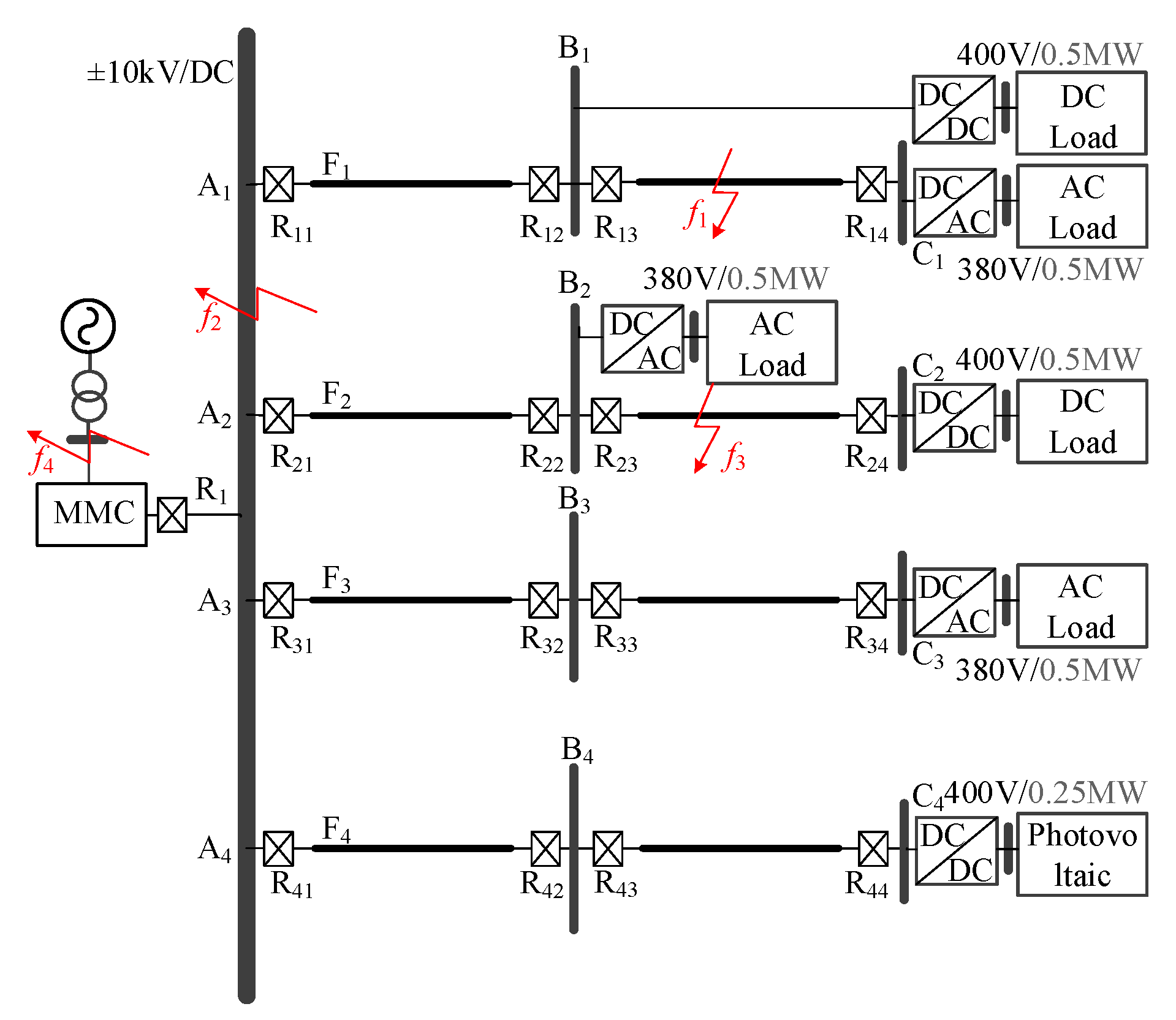
2.1. Radial MMC-MVDC Distribution Grid Topology

Compared with hand-in-hand and ring topologies, the radial DC distribution grid is widely adopted due to low investment. As shown in Figure 1, the system is composed by single MMC station which works in DC voltage control. 0.25 MW PV plant is boosted via a DC/DC converter into a ±10 kV DC busbar. The system parameters are shown in

Table 1. System parameters.

Parameters	Value
Voltage of AC system	110 kV
AC side rated voltage of MMC	10 kV
Rated active power of MMC	5 MW
Rated active power of photovoltaic	0.25 MW
Levels of converters	21
Capacitance of MMC	5000 μF
Inductance of bridge	5 mH

and the parameters of DC cable are shown in

Table 2. Parameters of feeder.

Parameters	Value
Resistance	0.125 Ω/km
Inductance	0.72 mH/km
Capacitance to ground	0.0048 μF/km
AmBm, BmCm (m = 1, 2, 3, 4)	10 km

.

2.2. Transient Analysis of DC Feeders

As a MMC-MVDC grid mostly utilizes the small current grounding modes [24], the voltage between two poles remains normal; thus, the system can still operate normally for a period of time. However, when a pole-to-pole fault occurs, the fault current rises rapidly and will bring the most serious hazard to the system. Therefore, this paper proposes the protection scheme mainly focusing on pole-to-pole fault. For a pole-to-pole fault occurring at f₁ in Figure 1, the frequency-domain fault superposition circuit schematic of the faulty feeder F₁ is shown in Figure 2.

Where, U_F represents the fault superimposed voltage source; Z_S represents the equivalent impedance of MMC; {ΔU₁, ΔI₁} represent the voltage fault component and the current fault component of the faulty feeder (F₁) at frequency ω; R_load is the equivalent load impedance; L is the current-limiting reactor installed at the beginning of the feeder; R_A1, L_A1, R_C1, and L_C1 are the equivalent resistances and inductances on both A₁ and C₁ sides, respectively. According to Figure 2, for a faulty feeder, when a pole-to-pole fault occurs on F₁, the voltage fault component and current fault component of faulty feeder meet the following relationship:

$$\frac{\Delta U_1}{\Delta I_1}=-Z_S$$

(1)

While for the normal feeders, the frequency-domain fault superposition circuit can be obtained according to the superposition principle as shown in Figure 3.

From Figure 3, it can be seen that the voltage fault component and current fault component of the normal feeders at the protection installation satisfy the following relationship:

$$\frac{\Delta U_k}{\Delta I_k}=j\omega L+R_{AkCk}+j\omega L_{AkCk}+R_{load}$$

(2)

where, k = 2, 3, 4, represents the feeder F₂, F₃, F₄; {ΔU_k, ΔI_k} represent the voltage fault component and the current fault component of the normal feeder (F_k) at frequency ω; R_AkCk, L_AkCk are equivalent resistances and inductances of the feeder A_kC_k, respectively. According to Equation (2), the phase difference of the voltage fault component and current fault component of the normal feeder should be between 0~90°.

However, the phase of Z_S cannot be directly determined. To solve this problem, the equivalent circuit of Z_S is constructed as shown in Figure 4. At this time, MMC is only paralleled by three phase units.

Where, L₀, C₀ represent the bridge reactance and submodule capacitors of MMC; R₀ is the equivalent resistance of the bridge arm; N is the number of submodules of bridge arm. To analyze the phase of Z_S, defining the equivalent impedance Z_C of the equivalent inductor and the equivalent capacitor as follows:

$$Z_C=j(\frac{2}{3}\omega L_0-\frac{N}{6\omega C_0})$$

(3)

Thus, the resonant frequency of the circuit is:

$$f_{res}=\frac{1}{4\pi }\sqrt{\frac{N}{L_0{C}_0}}$$

(4)

According to Equation (4), when $f>f_{res}$, Z_C > 0, Z_S is inductive. According to Table 1, $f>f_{res}=71.2 \mathrm{Hz}$. That is, when $f>71.2 \mathrm{Hz}$, the phase difference of voltage fault component and the current fault component of faulty feeder is between 180°~270°.

2.3. Transient Analysis of Feeder Segment

(1)

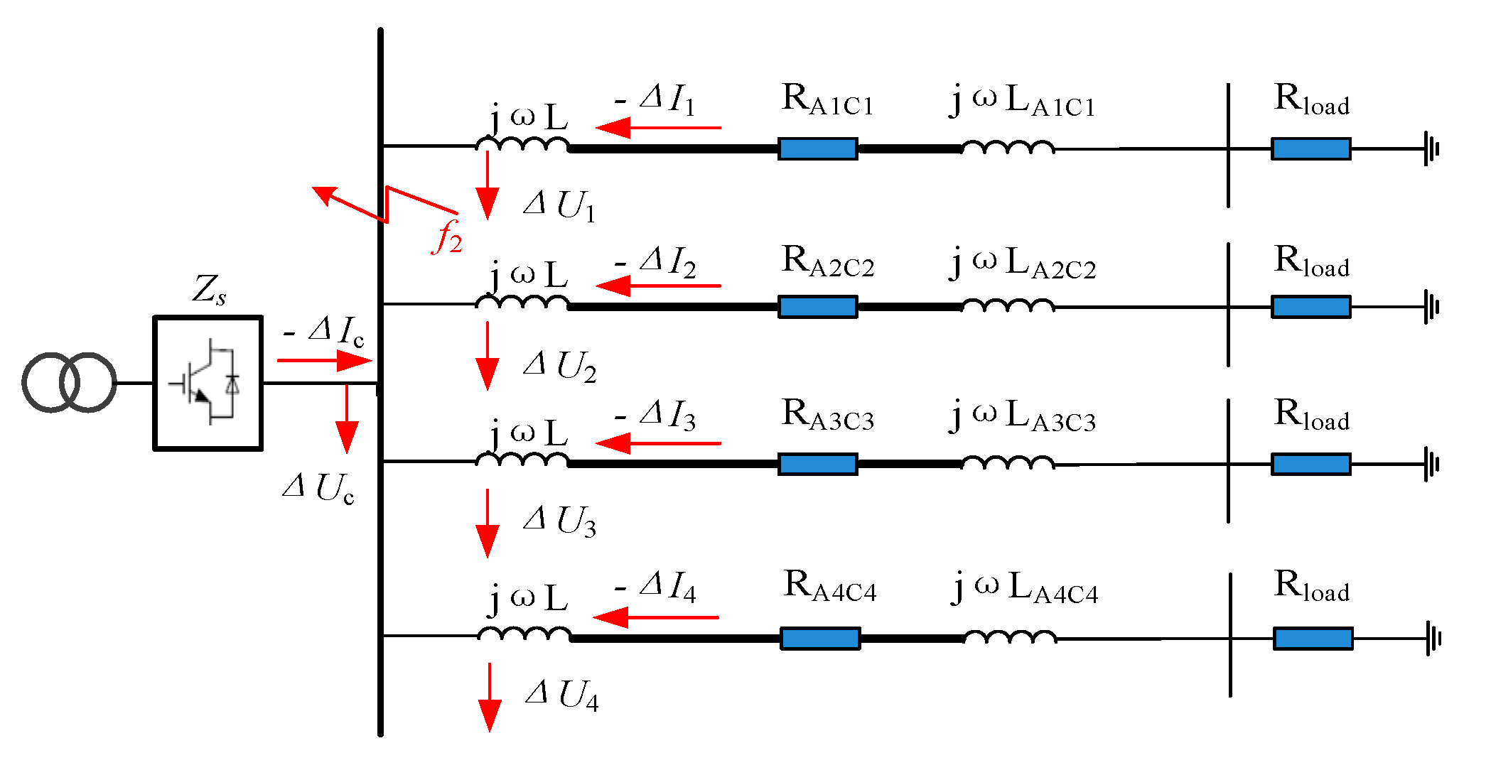
Internal fault of feeder segment: Take the fault at f₁ in Figure 1 as an example, when the internal fault occurs at f₁ for the segment B₁C₁, the superimposed circuit is illustrated as Figure 5. Assume the positive current direction is from busbar to the line for convenience. According to superposition principle, a negative voltage source ΔU_F is equivalent to be added at the fault point.

Where, Δ_IB1C1, Δ_IC1B1 respectively represent current fault components on both sides of segment B₁C₁. The load is generally connected to the DC busbar via a charging capacitor in the converters. Therefore, when the fault occurs at f₁, both sides feed current to the fault point. According to the specified positive direction, the current fault component detected by R₁₃ and R₁₄ should have the same polarity.

(2)

External fault of feeder segment: As there is no boundary between the segments of the same feeder, the current is almost not blocked from propagating between segment A₁B₁ and segment B₁C₁. Therefore, the polarities of the current fault component of the normal feeder detected by R₁₁ and R₁₂ are opposite.

2.4. Transient Analysis of Fault on the Bus

Specify the positive current direction is from the busbar to the line. When a pole-to-pole fault occurs on the DC busbar, the transient current characteristics can be illustrated as Figure 6. According to the analysis above, the voltage fault component and current fault component detected by the protection installation of feeder i and the converter satisfy the following relation:

$$\frac{\Delta U_i}{\Delta I_i}=j\omega L+R_{AiCi}+j\omega L_{AiCi}+R_{load}$$

(5)

$$\frac{\Delta U_c}{\Delta I_c}=Z_S$$

(6)

where, I = 1, 2, 3, 4, represents the feeder F₁–F₄; {ΔU_i, ΔI_i} represent the voltage fault component and the current fault component of the feeders at frequency ω; {ΔU_c, ΔI_c} represent the voltage fault component and the current fault component of the converter at frequency ω; R_AkCk, L_AkCk are equivalent resistances and inductances of the feeder A_kC_k, respectively. According to analysis above, the phase difference between the voltage fault component ΔU_i and current fault component ΔI_i of the normal feeders should be between 0~90°. In addition, the phase difference between the voltage fault component ΔU_c and current fault component ΔI_c of the converter should be between 0~90°.

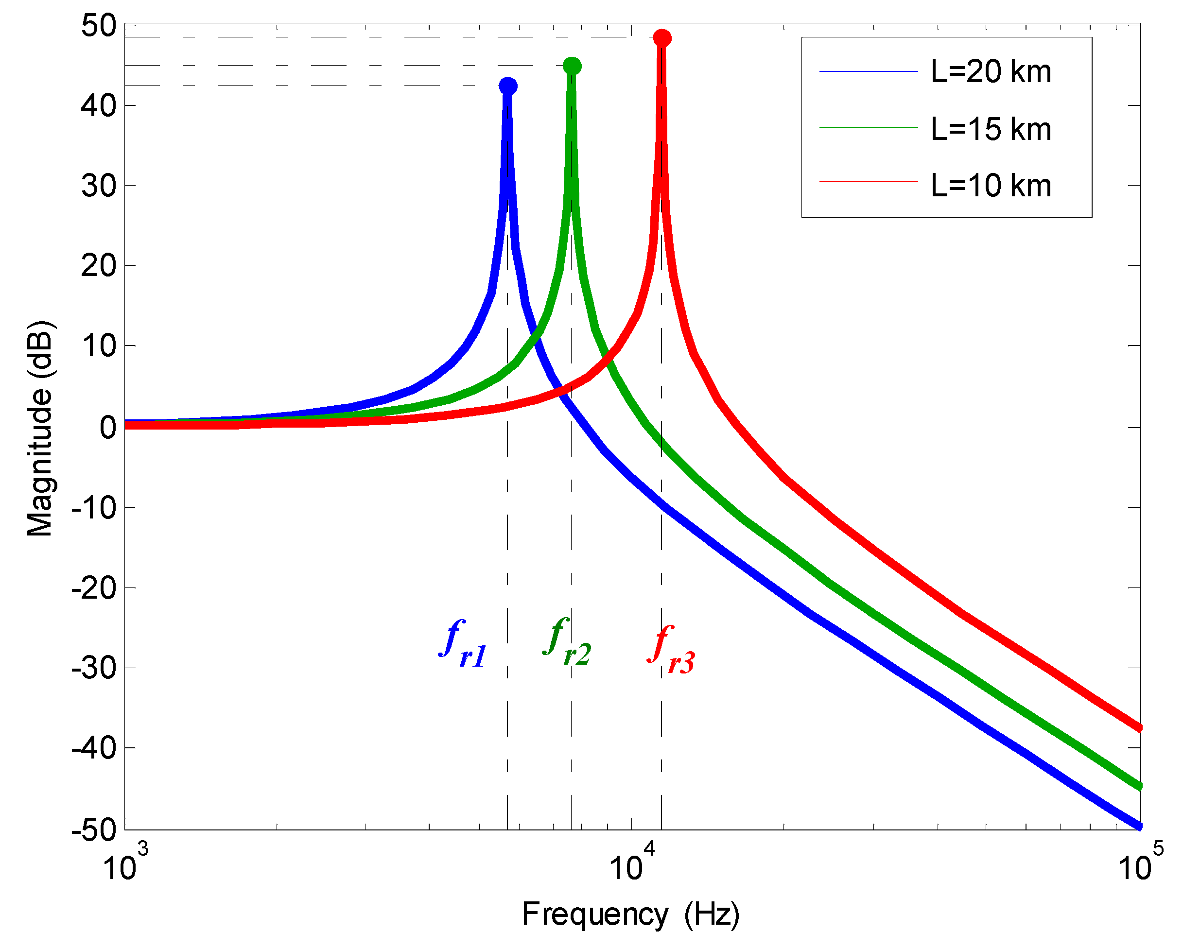
2.5. Analysis of Current Fault Component Characteristic Frequency Band

It can be seen from the analysis above that the faulty feeder and faulty segment can be identified by the characteristics of the current fault component. However, the current fault component of DC feeder is a continuous spectrum signal. The low-frequency band of the signal is susceptible to DC load currents, while the high-frequency signal will be rapidly attenuated due to the fast rise of impedance of feeder in the case of high-frequency band. Therefore, in order to extract the characteristic frequency band of current fault component effectively and improve the sensitivity of the criteria, the amplitude-frequency characteristics of the current fault component will be analyzed. As shown in Figure 7, DC feeder F₁ in Figure 1 is modelled by a π-type equivalent circuit, and the frequency characteristics of MMC-MVDC distribution grid are analyzed as follows.

According to the two-port network equation, the current-voltage relation in Figure 7 can be expressed as:

$$\{\begin{array}{l}{\dot{I}}_{p1}=(Y_1+Y_2){\dot{U}}_{p1}-Y_1{\dot{U}}_{L1}\\ {\dot{I}}_{L1}=Y_1{\dot{U}}_{p1}-(Y_1+Y_2){\dot{U}}_{L1}\end{array}$$

(7)

where, $\dot{I_{p_1}}$ and $\dot{U_{p_1}}$ denote the current and voltage at the beginning of F₁. ${\dot{I_L}}_1$ and ${\dot{U_L}}_1$ represent the current and voltage at the end of F₁. Y₁ and Y₂ are the admittance parameters of two-port network.

The transfer function between the current of beginning and end of the DC feeder is defined as follows:

$$G(S)={\frac{\stackrel{.}{I_{L1}(s)}}{\stackrel{.}{I_{p1}(s)}}|}_{\stackrel{.}{U_{L1}(s)}=0}$$

(8)

Substituting feeder parameters into Equation (8) and it can be given by:

$$G(s)=\frac{Y_1}{Y_2+Y_1}=\frac{2}{CL{l}^2{s}^2+CR{l}^{2}s+2}$$

(9)

where R, L and C denote the resistance, inductance and capacitance per unit length, respectively; l represents the length of the feeder.

The standard form of oscillation links of transfer function can be expressed as:

$$G^{\ast }(S)=\frac{1}{{(s/{\omega }_n)}^2+2\varsigma (s/{\omega }_n)+1}$$

(10)

The resonant angle frequency ${\omega }_r^{*}$ is given by:

$${\omega }_r^{\ast }={\omega }_n\sqrt{1-2{\varsigma }^2}$$

(11)

Substitute Equation (9) into the form of Equation (10), G(s) will be expressed as:

$$G(s)=\frac{1}{{(s/\sqrt{2/CL{l}^2})}^2+2(Rl\sqrt{C/8L})(s/\sqrt{2/CL{l}^2})+1}$$

(12)

$$\begin{array}{ccc}{\omega }_n=\sqrt{\frac{2}{CL{l}^2}}& ,& \zeta \end{array}=\frac{Rl}{2}\sqrt{\frac{C}{2L}}$$

(13)

Therefore, the resonant frequency f_r can be calculated as:

$$f_r={\omega }_r/2\pi =\sqrt{\frac{2}{CL{l}^2}-\frac{R^2}{2L^2}}/2\pi$$

(14)

According to the line parameters shown in Table 1, the amplitude-frequency curves of the transfer function G(s) can be obtained by substituting the different feeder lengths l = 20 km, 15 km and 10 km into Equation (12), respectively. The curves are shown in Figure 8.

According to Equation (14), the resonance frequencies f_r1 = 6054 Hz, f_r2 = 8072 Hz and f_r3 = 12,107 Hz are obtained respectively. It can be seen from Figure 8 that for the same line length, the amplitude A(ω) of the transfer function G(s) is gradually increased from 1 in the low frequency band range (0 < f < f_r); When f = f_r, the amplitude reaches the resonance peak and the line has the least attenuation effect on the current fault component. For the high frequency band (f > f_r), |A(ω)| decays rapidly from the resonant peak. When the length of the feeder reaches maximum length of 20km, ω_r reaches a minimum value of 6054 Hz. As the frequency increases from 6054 Hz, the attenuation effect on the current fault component will become stronger. In order to reduce the attenuation of the circuit, the frequency should not be greater than 6054 Hz. Meanwhile, as most of AC distributed power works in 50 Hz and most of DC distributed power works in low-frequency band, the low-frequency band of the fault component is easily affected by the load current and distributed power. Therefore, this paper selects characteristic frequency band between 500 Hz and 4000 Hz for analysis.

3. Application of S-Transform

S-transform has excellent time-frequency resolution characteristics. The height and width of Gaussian window changes with the variation of frequency. Based on good frequency resolution in the low frequency part and good time resolution in the high frequency part [25], it is very easy to extract the characteristic frequency band of current fault component using S-transform.

3.1. The S-Transform Theory

S transform is the development of wavelet transform and short-time Fourier transform [26], the S transform of a signal x(t) can be expressed as:

$$S(\tau ,f)={\displaystyle {\int }_{-\infty }^{+\infty }x(t)}\omega (\tau -t,f)e^{-i2\pi f\tau }dt$$

(15)

where, f and τ are the frequency-shift factor and time-shift factor; ω(τ − t, f) is Gaussian window function which can be defined as:

$$\omega (\tau -t,f)=\frac{\left|f\right|}{\sqrt{2\pi }}{e}^{-\frac{{(\tau -t)}^2{f}^2}{2}}$$

(16)

The S transform of a discrete signal x[kT] can be realized by the fast Fourier transform (letting $f\to n/NT$ and $\tau \to jT$):

$$\{\begin{array}{l}S[jT,\frac{n}{MT}]={\displaystyle \sum _{m=0}^{M-1}X[\frac{m+n}{MT}}]e^{-\frac{2{\pi }^2{m}^2}{n^2}}{e}^{\frac{i2\pi mj}{M}},n\ne 0\\ S[jT,0]=\frac{1}{M}{\displaystyle \sum _{m=0}^{M-1}x[\frac{m}{MT}}],n=0\end{array}$$

(17)

where k, j, m and n∈(0, M − 1). T is the sampling interval and M is the sampling number. $X\left[n/NT\right]$ denotes the discrete Fourier transform of x[jT] and $e^{-2{\pi }^2{m}^2/n^2}$ represents the Fourier spectrum of Gaussian window function.

3.2. S transform Characteristic Frequency Band (STCFB)

The S matrix obtained by S transform can be defined as S_a[p, q], where q is a column vector representing the amplitude-frequency characteristics of the signal at a sampling point, p is a row vector representing the time-domain characteristics of the signal at a certain frequency. Then STCFB of a signal at a certain time q can be defined as:

$$S[q]={\displaystyle \sum _{p=500}^{p=4000}S}[p,q]$$

(18)

where q = 1, 2…M. STCFB waveform can be drawn by calculating S[q] at each sampling point.

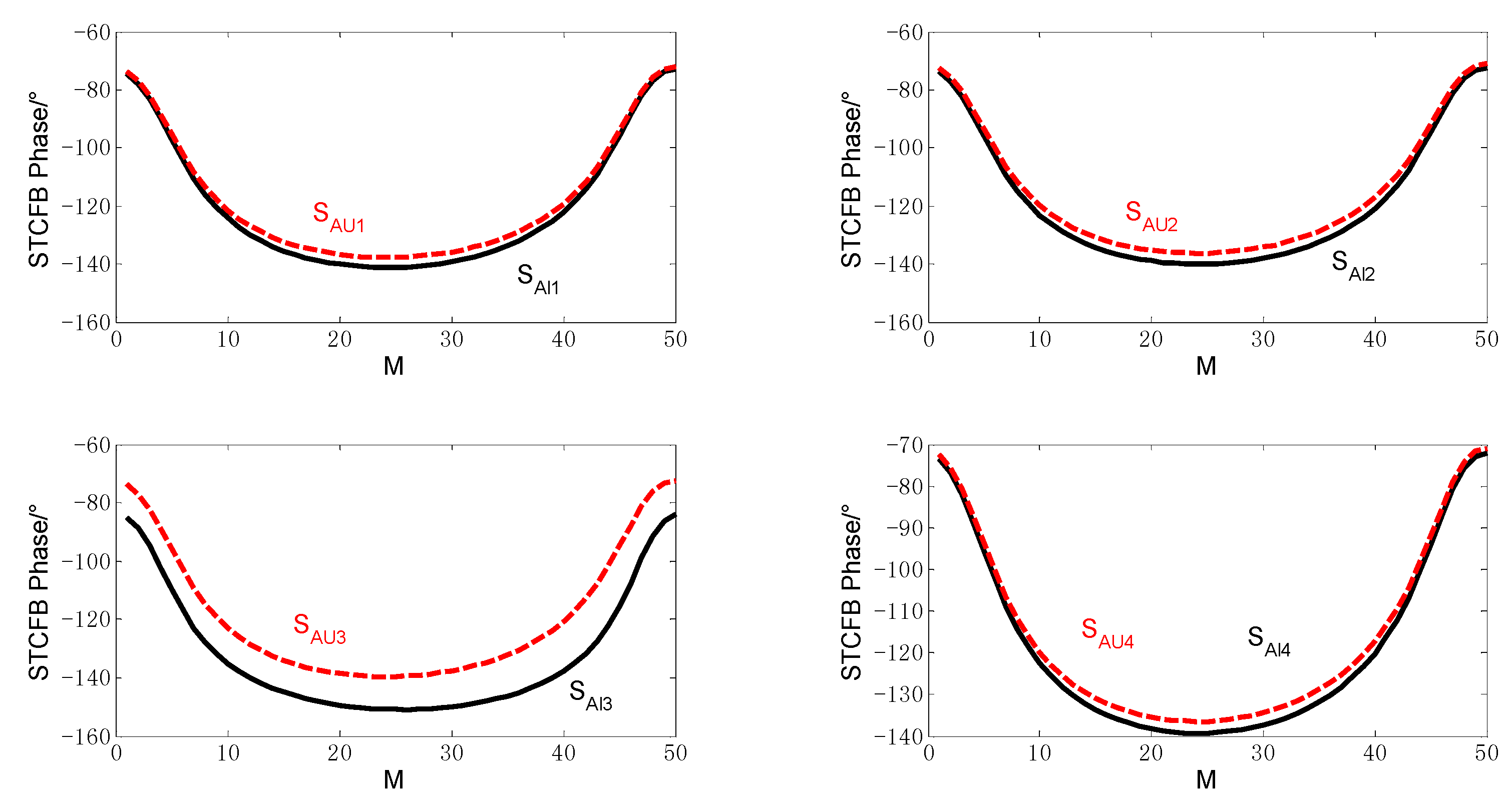
3.3. Analysis of STCFB Phase

In the matrix S_A[p, q], each element represents both of amplitude information and phase information of the signal at a particular frequency at a particular sampling point. The phase information extracted by single frequency has insufficient reliability and is also susceptible to interference signals. According to the analysis of the characteristic frequency band in the previous section, the STCFB Phase transformed from the signal S can be extracted as:

$$S_A[q]=angle(S[q])$$

(19)

where, S_A[q] is the phase of S[q], utilized to identify the faulty feeders and locate the faulty segments.

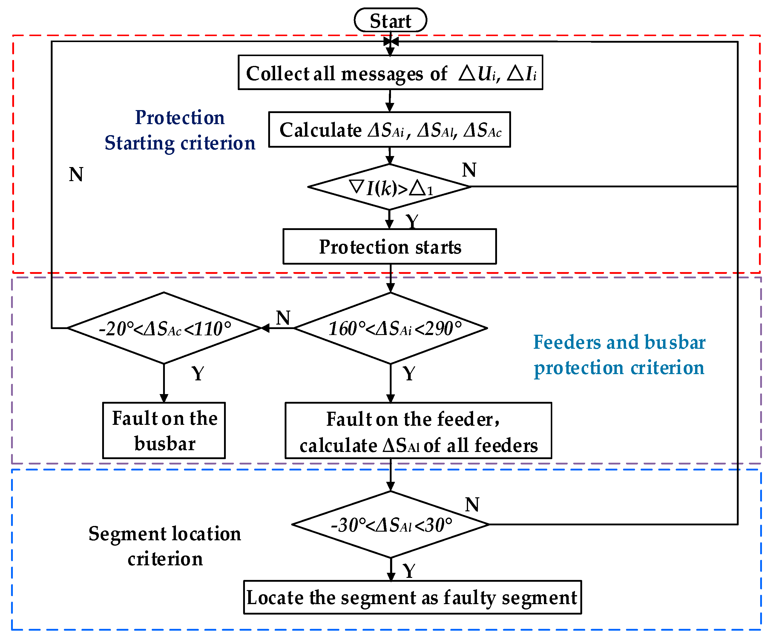
4. Protection and Location Scheme Based on S-Transform

4.1. Protection Starting Criterion

When MMC-MVDC system is in normal operation, the current fault component at the protection installation of DC distribution grid is almost zero. While the pole-to-pole fault occurs, the short circuit current at the protection installation of the line will rise rapidly. The current gradient is utilized to detect the abnormality since the system abnormality can be characterized by a current change [27], which can be expressed as:

$$\nabla I(k)=\frac{1}{3}{\displaystyle \sum _{i=0}^{2}I(k-i)-}\frac{1}{3}{\displaystyle \sum _{i=3}^{5}I(k-i)}$$

(20)

where, I(k-i) is the i-th sampling current value prior to the present moment; $\nabla I(k)$ is the calculated current gradient.

The start criterion of the protection is defined as:

$$\nabla I(k)>{\Delta }_1$$

(21)

where, Δ₁ is the starting threshold value. The value is greater than the maximum value of the current gradient during normal operation and switching load. According to the analysis and large simulations, Δ₁ = 5 A is obtained.

4.2. Protection Criterion on the Busbar and Feeders

According to the analysis above, it can be seen that in the characteristic frequency band, both the forward and backward impedance of the protection can be considered to be inductive. Therefore, after the protection starts, the busbar fault and feeder fault can be determined according to the STCFB Phase of voltage fault component and current fault component of feeders and the converter. When the protection starts, STCFB Phase difference of the voltage fault component and current fault component of feeders and the converter can be calculated based on the averaging method.

$$\Delta S_{Ai}=\frac{1}{M}{\displaystyle \sum _{q=1}^M|S_{AUi}(q)-S_{AIi}(q)|}$$

(22)

$$\Delta S_{Ac}=\frac{1}{M}{\displaystyle \sum _{q=1}^M|S_{AUc}(q)-S_{AIc}(q)|}$$

(23)

where, i = 1, 2, 3, 4, denotes four feeders; S_AUi(q) and S_AIi(q) are STCFB Phase of voltage fault component and current fault component at the q-th sampling point of the i-th feeder, respectively; S_AUc(q) and S_AIc(q) are STCFB Phase of voltage fault component and current fault component at the q-th sampling point of the converter; M is the number of sampling points in the data window. Theoretically, when the feeder i is a faulty feeder, the STCFB Phase difference between the two signals should be between 180° and 270°; On the other hand, when the feeder i is a normal feeder, the STCFB Phase difference between the two signals should be between 0°~90°. Considering the sensitivity and selectivity comprehensively, the criteria for identifying the faulty feeder can be constructed as follows:

$${160}^{\circ }<\Delta S_{Ai}<{290}^{\circ }$$

(24)

If Equation (24) is satisfied, the feeder i can be determined as faulty feeder.

The criterion for identifying the faulty busbar can be constructed as follows:

$$\{\begin{array}{l}-{20}^{\circ }<\Delta S_{Ai}<{110}^{\circ },i=1,2,3,4\\ -{20}^{\circ }<\Delta S_{Ac}<{110}^{\circ }\end{array}$$

(25)

If ΔS_Ai and ΔS_Ac satisfy the criterion in Equation (25), the pole-to-pole fault can be determined on the DC busbar.

4.3. Faulty Segment Location Criterion

On the basis of the characteristic analysis in Section 2.3, when an internal fault occurs on the segment, the STCFB Phase of current fault component on both sides of the segment are approximately the same; while the segment is faulty, the STCFB Phase on both sides of the segment are approximately opposite. Defining ΔS_Al as STCFB Phase difference of different feeder segments, then:

$$\Delta S_{Al}=\frac{1}{M}{\displaystyle \sum _{q=1}^M|S_{AIl}(q)-S_{AIr}(q)|}$$

(26)

where, S_AIl(q) and S_AIr(q) are the STCFB Phase of the current fault component at the q-th sampling point on both sides of the segment. The faulty segment location criterion can be constructed as follows:

$$-{30}^{\circ }<\Delta S_{Al}<{30}^{\circ }$$

(27)

When Equation (27) is satisfied, the faulty segment is determined. Otherwise, it is judged as a normal segment.

4.4. Flow Chart of Protection and Location Scheme

Based on the analysis above, the flow chart of protection and segment location scheme shown in Figure 9 can be designed based on the protection starting criterion, feeders and busbar protection criterion, and segment location criterion.

5. Simulation and Analysis

In order to validate the proposed protection and location criteria, a ±10 kV natural bipolar radial MMC-MVDC simulation model was built in Figure 1. The pole-to-pole faults are set at different fault locations to test the reliability of the method. The protection units (R₁₁, R₁₂, R₁₃, R₁₄, R₂₁, R₂₂, R₂₃, R₂₄, R₃₁, R₃₂, R₃₃, R₃₄, R₄₁, R₄₂, R₄₃, R₄₄, and R₁) are located as shown in the figure. The entire data window is 2ms in length and the sampling frequency is 25 kHz.

5.1. Metallic Pole-to-Pole Fault

Setting a metallic pole-to-pole fault at f₁ in the middle of segment B₁C₁, the STCFB Phase of current and voltage fault component of all feeders are shown in Figure 10. The results are indicated in

Table 3. Simulation results of STCFB (S-transform characteristic frequency band) Phase difference for the fault at f_1.

ΔSAi(°)				Simulation Results
F1	F2	F3	F4
188.461	6.435	7.055	6.492	Fault on F1

.

Where, {S_AUi, S_AIi} represents the STCFB Phase of voltage fault component and current fault component of feeder F₁–F₄. ΔS_Ai is the phase difference of voltage fault component and current fault component of all feeders. According to Figure 10 and Table 3, the STCFB Phase difference of voltage fault component and current fault component on the head of F₁ is 188.461°. While the STCFB Phase difference of voltage fault component and current fault component on the head of F₂, F₃, and F4 are 6.435°, 7.055°, 6.492°. Thus, F₁ can be determined as the faulty feeder.

Further analyzing STCFB Phase on both sides of segment A₁B₁ and B₁C₁, the waveforms are shown in Figure 11 and the simulation results are indicated in

Table 4. Simulation results of STCFB Phase difference for the segment A₁B₁ and B₁C₁.

ΔSAl (°)		Simulation Results
A1B1	B1C1
180.723	1.671	Fault on B1C1

.

Where, {S_AA1B1, S_AB1A1}, {S_AB1C1, S_AC1B1} represent the STCFB Phase on both sides of segment A₁B₁ and B₁C₁; ΔS_Al is the STCFB Phase difference on both sides of segment A₁B₁ and B₁C₁. As shown in Figure 11 and Table 4, the STCFB Phase difference of voltage fault component and current fault component on both sides of A₁B₁ is 180.723°. While the STCFB Phase difference of voltage fault component and current fault component on both sides of B₁C₁ is 1.671°. Thus, B₁C₁ can be identified as the faulty segment.

5.2. Metallic Bus Fault

A metallic fault is set at f₂ on the busbar as shown in Figure 1. At this time, $\nabla I(k)$ is 25 A, and the protection starts. The STCFB Phase of voltage fault component and current fault component for four feeders are shown in Figure 12. The simulation results are indicated in

Table 5. Simulation results of fault on the busbar.

ΔSAc (°)	ΔSAi (°)				Simulation Results
	F1	F2	F3	F4
25.613	2.647	3.258	13.495	2.480	Fault on f2

.

According to Figure 12 and Table 5, the STCFB Phase difference of voltage fault component and current fault component at the head of F₁, F₂, F₃, F₄ is 2.647°, 3.258°, 13.495°, and 2.480°. The STCFB Phase difference of voltage fault component and current fault component of the converter is 25.613°. Therefore, the fault is determined on the busbar.

5.3. Simulation for Influencing Factors

In order to verify the reliability of the proposed protection and location criterion under different factors, extensive simulations were performed as follows.

(1)

Fault on the feeder under different fault resistances: Faults under different resistances are set at f₁ in the middle of segment B₁C₁. The simulation results of feeders are indicated in

Table 6. Simulation results of faulty feeders under different fault resistances.

Resistance/Ω	ΔSAi (°)				Simulation Results
	F1	F2	F3	F4
20	189.713	7.124	7.253	7.053	Fault on F1
50	190.541	7.521	8.552	7.535	Fault on F1

. The results of segments are indicated in

Table 7. Simulation results of faulty segments under different fault resistances.

Resistance/Ω	ΔSAl (°)		Simulation Results
	A1B1	B1C1
20	182.194	7.405	Fault on B1C1
50	183.052	7.704	Fault on B1C1

.

On the basis of Table 6 and Table 7, F₁ can be selected as faulty feeder under different resistances. In addition, segment B₁C₁ can be correctly located.

(2)

Simulation of fault on the busbar under different fault resistances:

Faults with different transition resistances are set at f₂ on the busbar. The identification results are shown in

Table 8. Simulation results of faulty busbar under different fault resistances.

Resistance/Ω	ΔSAc（°）	ΔSAi (°)				Simulation Results
		F1	F2	F3	F4
20	22.124	1.672	9.860	16.178	21.799	Fault on busbar
50	20.118	1.276	7.986	12.552	19.637	Fault on busbar

.

As the results shown in Table 8, the fault on the busbar can be correctly determined under different resistances. The results show that the resistance has little impact on the criteria.

(3)

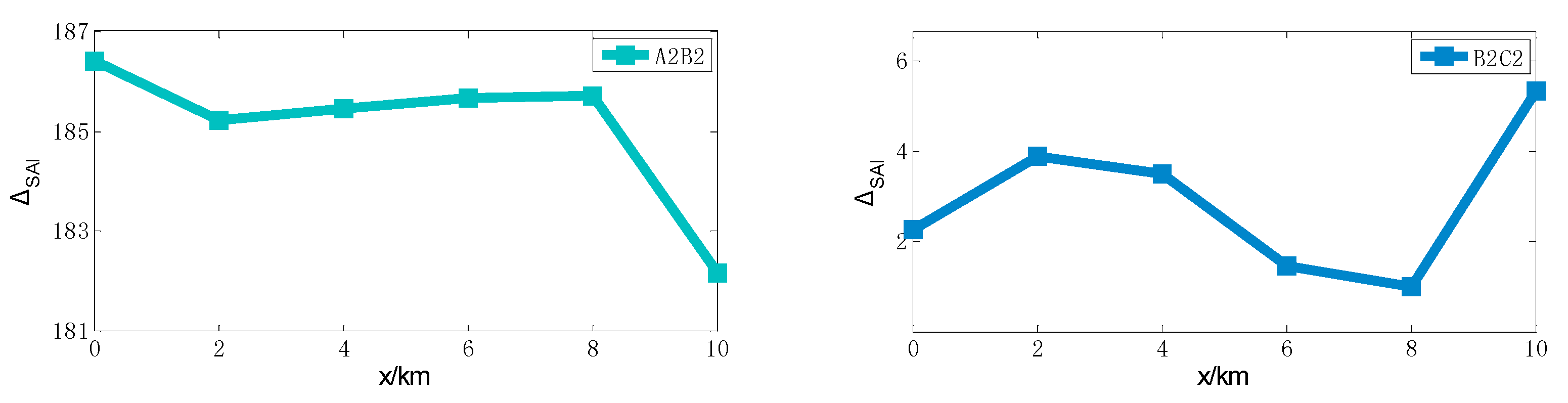
Simulation of different fault locations: Set the pole-to-pole fault at f₃ and take the transition resistance as 20Ω. The simulation results of STCFB Phase difference on both sides of segment A₂B₂ and B₂C₂ are shown in Figure 13. The abscissa indicates the distance from the fault point to A₂.

According to Figure 13, when the fault occurs on different locations of the segment, the faulty segment can be correctly located, and the sensitivity is high.

(4)

Noise: The noise interferences will be doped in the voltage and current fault component, which will easily cause maloperation of protection. Therefore, Gaussian white noise with different decibels is added to the voltage and current fault component signals. The simulation results are shown in

Table 9. Simulation results of feeder under different Gaussian noise.

Gaussian Noise/dB	ΔSAi (°)				Simulation Results
	F1	F2	F3	F4
30	188.697	7.505	9.208	7.532	Fault on F1
40	188.758	6.695	6.901	6.368	Fault on F1
80	188.458	6.437	7.050	6.487	Fault on F1

.

On the basis of the simulation results above, it can be seen that the scheme is hardly affected by noise.

(5)

Fault on AC side: Different types of pole-to-pole faults are set at f₄ on the AC busbar. According to the simulation, during the entire transient process, $\nabla I(k)$ < Δ₁ is always satisfied. Therefore, the protection does not start, and the system can still operate normally.

6. Conclusions

Due to the existing protection and location scheme mainly focus on HVDC grid and LVDC grid, a novel protection and location method was firstly proposed for MMC-MVDC grid. Considering the transient characteristics of MMC-MVDC distribution grids, the scheme can be divided into three stages, namely: (1) Protection starting criterion; (2) feeders and busbar protection criterion, and (3) segment location criterion. Utilizing PSCAD/EMTDC software, a radial MMC-MVDC distribution grid was constructed and extensive simulations were realized. From the theoretical analysis and simulation results, the following conclusions could be drawn:

(1)

The simulation results show that influencing factors such as the fault resistance, the noises and fault position, can hardly affect the correct operation of the proposed criteria.

(2)

Utilizing the non-unit data and the data window of 2 ms to protect the feeder and the busbar, the protection is fast and reliable.

(3)

The criteria only utilizes the current and voltage fault component to protect the system and locate the fault, which is adaptable in the intricate topologies.

References

1. Bukhari, S.; Zaman, M.; Haider, R.; Oh, Y.; Kim, C. A protection scheme for microgrid with multiple distributed generations using superimposed reactive energy. Int. J. Electr. Power Energy Syst. 2017, 92, 156–166. [Google Scholar] [CrossRef]
2. Li, X.; Cui, X.; Lu, T.; Wang, D.; Ma, W.; Bian, X. Comparison between the audible noises generated from single corona source under DC and AC corona discharge. CSEE JPES 2015, 1, 23–30. [Google Scholar]
3. Techakittiroj, K.; Wongpaibool, V. Co-existance between AC-Distribution and DC-Distribution: In the View of Appliances. Available online: http://repository.au.edu/bitstream/handle/6623004553/17921/Proceeding-Paper-Abstract-17921.PDF?sequence=2&isAllowed=y (accessed on 8 August 2018).
4. Xue, S.; Gao, F.; Sun, W.; Li, B. Protection Principle for a DC Distribution System with a Resistive Superconductive Fault Current Limiter. Energies 2015, 8, 4839–4852. [Google Scholar] [CrossRef] [Green Version]
5. Mehrasa, M.; Pouresmaeil, E.; Zabihi, S.; Caballero, J.C.T.; Catalão, J.P.S. A Novel Modulation Function-Based Control of Modular Multilevel Converters for High Voltage Direct Current Transmission Systems. Energies 2016, 9, 867. [Google Scholar] [CrossRef] [Green Version]
6. Mehrasa, M.; Pouresmaeil, E.; Zabihi, S; Vechiu, I.; Catalão, J.P.S. A multi-loop control technique for the stable operation of modular multilevel converters in HVDC transmission systems. Int. J. Electr. Power Energy Syst. 2018, 96, 194–207. [Google Scholar] [CrossRef]
7. Mehrasa, M.; Pouresmaeil, E.; Zabihi, S.; Catalão, J.P.S. Dynamic Model, Control and Stability Analysis of MMC in HVDC Transmission Systems. IEEE Trans. Power Deliv. 2017, 32, 1471–1482. [Google Scholar] [CrossRef]
8. Mehrasa, M.; Pouresmaeil, E.; Taheri, S.; Vechiu, I.; Catalão, J.P.S. Novel Control Strategy for Modular Multilevel Converters Based on Differential Flatness Theory. IEEE J. Emerg. Sel. Top. Power Electron. 2018, 6, 888–897. [Google Scholar] [CrossRef]
9. Sun, G.; Shi, B.; Zhao, Y.; Li, S. Research on the fault location method and protection configuration strategy of MMC based DC distribution grid. Power Syst. Prot. Control 2015, 43, 127–133. [Google Scholar]
10. Xue, S.M.; Liu, C. Line-to-Line Fault Analysis and Location in a VSC-Based Low-Voltage DC Distribution Network. Energies 2018, 11, 536. [Google Scholar] [CrossRef]
11. Jamali, S.Z.; Bukhari, S.B.A.; Khan, M.O.; Mehdi, M.; Noh, C.H.; Gwon, G.H.; Kim, C.H. Protection Scheme of a Last Mile Active LVDC Distribution Network with Reclosing Option. Energies 2018, 11, 1093. [Google Scholar] [CrossRef]
12. Chaudhuri, N.R.; Chaudhuri, B.; Majumder, R.; Yazdani, A. Multi-Terminal Direct-Current Grids: Modeling, Analysis, and Control; Wiley-IEEE Press: Hoboken, NJ, USA, 2014. [Google Scholar]
13. Mehrasa, M.; Pouresmaeil, E.; Akorede, M.F.; Zabihi, S.; Catalão, J.P.S. Function-based modulation control for modular multilevel converters under varying loading and parameters conditions. IET Gener. Transm. Distrib. 2017, 11, 3222–3230. [Google Scholar] [CrossRef]
14. Azizi, S.; Afsharnia, S.; Sanaye-Pasand, M. Fault location on multi-terminal DC systems using synchronized current measurements. Int. J. Electr. Power Energy Syst. 2014, 63, 779–786. [Google Scholar] [CrossRef]
15. Zhang, S.; Zou, G.B.; Huang, Q.; Gao, H. A Traveling-Wave-Based Fault Location Scheme for MMC-Based Multi-Terminal DC Grids. Energies 2018, 11, 401. [Google Scholar] [CrossRef]
16. Leterme, W.; Beerten, J.; Hertem, D.V. Nonunit Protection of HVDC Grids with Inductive DC Cable Termination. IEEE Trans. Power Deliv. 2016, 31, 820–828. [Google Scholar] [CrossRef]
17. Baran, M.E.; Mahajan, N.R. Overcurrent Protection on Voltage-Source-Converter-Based Multi-terminal DC Distribution Systems. IEEE Trans. Power Deliv. 2007, 22, 406–412. [Google Scholar] [CrossRef]
18. Xue, S.M.; Chen, C.C.; Yi, J.; Li, B.; Wang, Y. Protection for DC Distribution System with Distributed Generator. J. Appl. Math. 2014, 2014, 1–12. [Google Scholar] [CrossRef]
19. Feng, X.; Li, Q.; Pan, J. A novel fault location method and algorithm for DC distribution protection. IEEE Trans. Ind. Appl. 2017, 53, 1834–1840. [Google Scholar] [CrossRef]
20. Tang, L.; Ooi, B.T. Locating and Isolating DC Faults in Multi-Terminal DC Systems. IEEE Trans. Power Deliv. 2007, 22, 1877–1884. [Google Scholar] [CrossRef]
21. Zheng, X.; Tai, N.; Wu, Z.; Thorp, J. Harmonic current protection scheme for voltage source converter-based high-voltage direct current transmission system. IET Gener. Transm. Distrib. 2018, 8, 1509–1515. [Google Scholar] [CrossRef]
22. Yang, J.; Fletcher, J.E.; O’Reilly, J. Multi terminal DC Wind Farm Collection Grid Internal Fault Analysis and Protection Design. IEEE Trans. Power Deliv. 2010, 25, 2308–2318. [Google Scholar] [CrossRef]
23. Sneath, J.; Rajapakse, A.D. Fault Detection and Interruption in an Earthed HVDC Grid Using ROCOV and Hybrid DC Breakers. IEEE Trans. Power Deliv. 2016, 31, 973–981. [Google Scholar] [CrossRef]
24. Song, G.B.; Luo, J.; Gao, S.P.; Wang, X.; Tassawar, K. Detection method for single-pole-grounded faulty feeder based on parameter identification in MVDC distribution grids. Int. J. Electr. Power Energy Syst. 2018, 97, 85–92. [Google Scholar] [CrossRef]
25. Zhao, P.; Chen, Q.; Sun, K.; Xi, C. A Current Frequency Component-Based Fault-Location Method for Voltage-Source Converter-Based High-Voltage Direct Current (VSC-HVDC) Cables Using the S Transform. Energies 2017, 10, 1115. [Google Scholar] [CrossRef]
26. Stockwell, R.G.; Mansinha, L.; Lowe, R.P. Localization of the complex spectrum: the S transform. IEEE Trans. Signal Process. 1996, 44, 998–1001. [Google Scholar] [CrossRef] [Green Version]
27. Kong, F.; Hao, Z.; Zhang, S.; Zhang, B. Development of a Novel Protection Device for Bipolar HVDC Transmission Lines. IEEE Trans. Power Deliv. 2014, 29, 227–2278. [Google Scholar] [CrossRef]
Figure 1. Radial Modular Multilevel Converter-Medium Voltage Direct Current (MMC-MVDC) distribution grid topology.
Energies 11 02076 g001
Figure 2. Frequency-domain fault superposition circuit of faulty feeder.
Energies 11 02076 g002
Figure 3. Frequency-domain fault superposition circuit of normal feeders.
Energies 11 02076 g003
Figure 4. Equivalent Circuit of Pole-to-Pole Fault on MMC
Energies 11 02076 g004
Figure 5. Frequency-domain fault superposition circuit for an internal fault.
Energies 11 02076 g005
Figure 6. Frequency-domain fault superposition circuit for a pole-to-pole fault on the busbar.
Energies 11 02076 g006
Figure 7. π-type equivalent circuit.
Energies 11 02076 g007
Figure 8. Amplitude-frequency characteristics of DC feeder.
Energies 11 02076 g008
Figure 9. Flow chart of protection and location scheme for pole-to-pole fault.
Energies 11 02076 g009
Figure 10. S-transform characteristic frequency band (STCFB) Phase of faulty feeder under pole-to-pole fault.
Energies 11 02076 g010
Figure 11. STCFB Phase on both sides of segment A1B1 and B1C1.
Energies 11 02076 g011
Figure 12. STCFB Phase on both sides of segment A1B1 and B1C1.
Energies 11 02076 g012
Figure 13. STCFB Phase of faults on different locations in the segment A2B2 and B2C2.
Energies 11 02076 g013