Abstract
In a photovoltaic solar-vehicle system, many factors may present disturbances and thus affect its operation. Among the disturbing parameters are the variable output voltage of the photovoltaic generator (GPV) and unbalanced irradiation throughout a day, as well as both the variable load (considered as a resistor in our case) and duty cycle. For a better quality output voltage, the optimization of the transfer power, and the protection of the photovoltaic solar vehicle system, the following is required: a constant and non-oscillating tension in the continuous bus and the extraction of the maximum power generated by the photovoltaic array under variable climatic conditions, as well as a specific model of boost converter. This paper discusses the optimization of the transfer power between the photovoltaic array and load in the first step, the study of an average model of the direct current/direct current (DC/DC) converter, and finally the design of a stable and robust tension controller. The results achieved confirm the rightness of the proposed control structure, which is simple, robust, and can secure the stability and good quality dynamics of the controlled system, as well as ensure invariance against disturbances. Also, the average model of the DC/DC converter used was found to be efficient.
1. Introduction
The significant growth of modern cities has led to the increased the use of transport, which has led to increased pollution and other serious environmental problems affecting the health of living beings. Another problem is the gases produced by the vehicles; this need to be minimized by the control of emissions and the implementation of proactive measures. In this context, the car industry has introduced solar electric vehicles to minimize the use of combustion engines by replacing them with electric motors. Solar electric vehicles powered by renewable energies offer a solution to develop zero-emission motor vehicles because they emit only natural byproducts and not exhaust fumes, which improves air quality in cities and therefore improves the health of their populations.
In Reference [1], Amari et al., proposed a new high-frequency unidirectional direct current/direct current (DC/DC) converter. The two levels of voltage converter were altered by a full bridge inverter composed of two planar transformers in high frequency. This solution presented the possibility to minimize the switching losses, the size, and the weight of the converter. In Reference [2], a new bidirectional DC/DC converter was proposed. The author presented an average model of this DC/DC converter, which was used to calculate the transient characteristics of the converter. In order to gain the desired voltage in a closed loop under load, the output and the input voltages were regulated with an implemented proportional–integral (PI) controller. The input voltage variations were characterized by a short response time. In both of the above works, the power sources were fuel cells, which are non-polluting, very energy efficient, silent, and require little maintenance.
However, these cells have the following drawbacks:
- -
- A high cost, which remains the major obstacle to their marketing, because their construction uses expensive materials.
- -
- A lifetime that poses big question marks. Today, it is only a few thousand hours, while it must reach a life of 20,000 to 40,000 h (between 2 and 5 years).
- -
- The unavailability of fuels of adequate quality.
In Reference [3], an original proportional Integral Fuzzy-Logic controller was proposed by Sarkar et al., which increases the range of the solar car by improving its energy management. In this work, the author assumed that the meteorological conditions are relatively favorable, which is not always the case.
The Electric Power System design and development of an electric solar vehicle are presented in Reference [4].
An integrated MPPT (maximum power point tracking) algorithm is used by the power system to simultaneously extract the energy from the photovoltaic panels and to control the charge of the battery. The design methodology presented in this work is for race vehicles; however, it could be used for commercially vehicles as well.
In the present work, we demonstrate a photovoltaic electric-vehicle system whose overall diagram is illustrated in Figure 1. Our system ensures the optimization of energy transfer between the photovoltaic generator (GPV) and the load. Also, it provides a fault tolerance mechanism through the specific DC/DC boost topology.
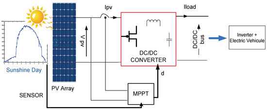
Figure 1.
Diagram of the (photovoltaic) electric-vehicle system. PV: photovoltaic; MPPT: maximum power point tracking; DC/DC: direct current/direct current.
This research is divided into three sections. First, the effects of the irradiation on the performance of the power solar generation are determined. Second, the numerical method (MPPT) based on least squares is used to improve the impact of unbalanced climatic conditions on the dynamic behaviour of the system. Third, we discuss the topology of the power interface used in order to optimize the transfer of the power generated by the photovoltaic array to the DC/DC bus throughout a day.
Finally, the simulations results obtained over one day describe the behaviour of our system under unbalanced climatic conditions.
2. Photovoltaic Generator Modeling
The electrical model and parameters of the solar cell are illustrated in Figure 2.
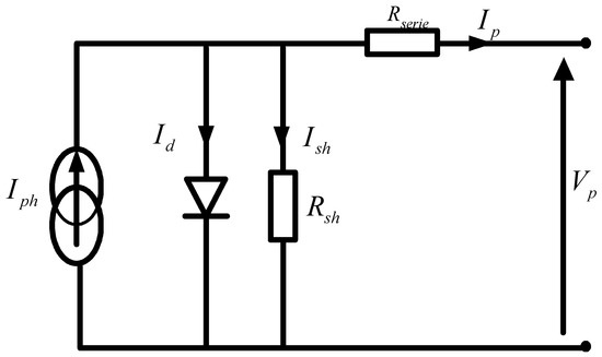
Figure 2.
Photovoltaic cell equivalent circuit.
Equation (1) described the relationship between the output current and the voltage across a photovoltaic cell [5,6,7,8].
where and are the output current and output voltage of the solar cell, respectively. is the thermodynamic potential of the cell, q: is the charge of an electron, is the Boltzmann’s constant, is the ideality factor for a p-n junction, and T is the temperature of the solar cell . is the generated current under a given irradiation and is the saturation current of the diode.
The relationship between the PV (photovoltaic) array output current and the voltage is given by Equation (2).
where prepresents the current delivered by the parallel cells; is the voltage produced across the photovoltaic generator composed by series cells.
In Table 1, the characteristics of photovoltaic generator used in our work are shown.

Table 1.
Photovoltaic module parameters.
Figure 3 and Figure 4 show that irradiation essentially affects the current generated by the photovoltaic generator.
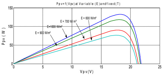
Figure 3.
Variation of the photovoltaic generator (GPV) power and voltage, for different values of the illumination at a fixed temperature.
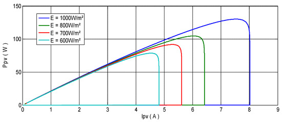
Figure 4.
Variation of the GPV power and current, for different values of the illumination at a fixed temperature.
3. Maximum Power Point Tracking Algorithm
As previously indicated, the irradiation variation significantly affects the photovoltaic cell output current; however, this irradiation has no impact on the voltage cell. In addition, the variation range of the photovoltaic cell temperature is very limited [6,9,10]. In order to extract the maximum power, the photovoltaic voltage has to be controlled by the maximum power point (MPP).
Many techniques that are available depend on cost, hardware implementation, sensors, and speed. The recommended numerical MPPT controls used in this work is the least squares method. This technique was used to simulate our system under a constant temperature and variable irradiation throughout a day.
This unbalanced illumination during one day is illustrated by the following figure (Figure 5).
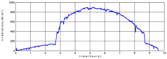
Figure 5.
Variation of the illumination during a day in Tunis (Tunisia) on 5 April 2012.
Equations (3) and (4), which manage the least squares MPPT approach, are given as follows:
where is the degree of the polynomial; and are the constants of the polynomial; and is the optimal duty cycle. The resulting fits of the curves characteristic of GPV using this method are displayed in Figure 6.
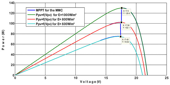
Figure 6.
Trajectory of maximum power point of the photovoltaic generator.
4. Average Model of the DC/DC Converter
4.1. Topology of the Converter
The schematic representation of the converter associated with the photovoltaic panel is illustrated in Figure 7. The phase number of this converter was chosen based on four criteria, including the reduction of the volume of the inductors, the reduction of the root mean square (RMS) current of the output capacitor, and energy efficiency. Due to the natural static redundancy of this topology, healthy phases can be used in the event of power switch faults, for example the use of a compensation system, thus avoiding the interruption of the power supply.
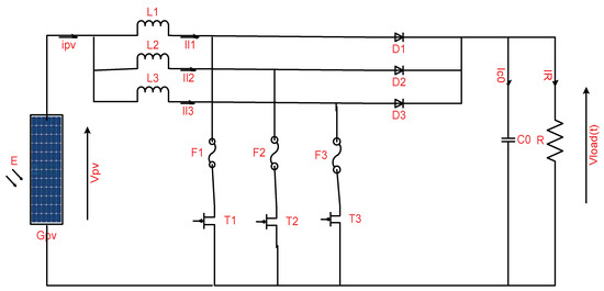
Figure 7.
Topology of the converter.
In order to meet the requirements of the fault tolerance, fuses (F1, F2, and F3) were added in series with each power switch. The fuses are used to isolate the faulty phase in the case of short circuit faults in the power switches.
To facilitate the study, the load was considered to be a resistive load. This unidirectional DC/DC converter was based on three MOSFETs (Metal Oxide Se miconductor Field Effect Transistor) (T1, T2, and T3) and three diodes (D1, D2, and D3), in addition to the smoothing coils (L1, L2, and L3), the filter capacitor of the voltage output (Vload), and the input voltage delivered by the photovoltaic generator (Vpv).
4.2. Operation of the Converter
Figure 8 shows the operation mode of the converter, which contains three cycles:
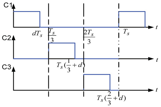
Figure 8.
Operating waveforms of the switches.
C1, C2, and C3 respectively denote the control signals of the MOSFETs.
Ts and d represent the switching period and the controlled duty ratio.
4.3. Mathematical Model of the Converter
To study the average model, we choose four state variables, iL1, iL2, iL3 and V0 as shown in Figure 7. The state space representation of the system is:
with , , and .
We are interested to studied the converter if .
This mode consists of six steps (see Figure 9), which are the states of the switches given by the following chronograms and recapped in Table 2.
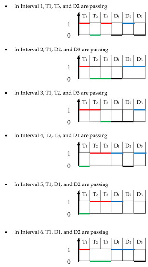
Figure 9.
Chronograms of the stats switches.
Table 2.
Recap of the stats switches.
The recap of the full states of the switches of the model are illustrate in Table 2.
The equivalents schemas of the states of switches over the six intervals of the considered model in Figure 10.
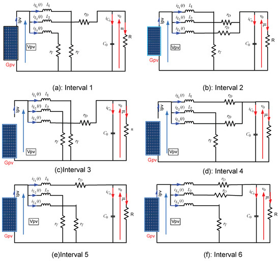
Figure 10.
Equivalents schemas of the states of switches over the six intervals.
If we apply Kirchhoff’s law, we can obtain the system of the equations developed in the Appendix.
The matrix notations of these equations are:
During the switching period, the average model state can be obtained as the following:
with
5. Small Signal
The variables were analyzed to direct components (upper case letter) and a small alternating current (AC) perturbation (represented by (~)).
The equilibrium point of the DC/DC converter is given by:
Substituting Equation (6) into Equation (5) yields:
If we neglect the products of the terms , we obtain:
Using Laplace transforms for Equation (10):
We can define the transfer function of the output voltage to the duty cycle:
with
where p is the Laplace operator.
6. Open Loop System Study
The characteristics of the equilibrium point are the output voltage (V0) and the output current (IL). Indeed, these characteristics could be determined with the input voltage, the resistor, and the duty cycle (Vpv = 24 V, R = 10 Ω and d = 0.37).
The average model state is:
We pose
At equilibrium we have
So
The output voltage and the current at equilibrium are confirmed by simulations, as shown in Figure 11 and Figure 12.
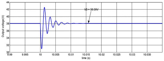
Figure 11.
Output voltage at equilibrium.
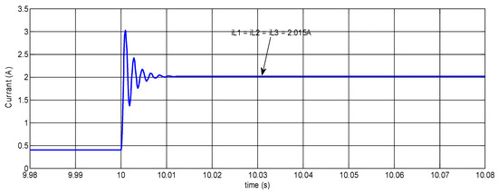
Figure 12.
Output current at equilibrium.
We noticed that the output voltage and current require about 0.010 s to stabilize. This result allowed us to discern that this converter exhibits high precision.
In the following, we present the simulation results of the photovoltaic electric-vehicle system in an open loop under different scenarios.
• Scenario 1:
R = 10 Ω, d = 0.66, and a variable input voltage converter.
Figure 13 shows the unbalanced irradiation and the photovoltaic voltage over one day. Figure 14 shows the proportional responses of the proposed average DC/DC converter.
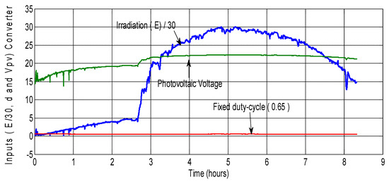
Figure 13.
Inputs (d, Vpv, and E) into the converter vs. time.
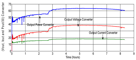
Figure 14.
Outputs (V0, iL, and power) from the converter vs. time.
We note that the bivariate polynomial is used for the simulation of the system where both irradiation and temperature are variable.
In stand-alone photovoltaic power systems, the output voltage is effectively a constant DC bus (Figure 14 with red color).
• Scenario 2:
R = 10 Ω, Vpv = 24 V, and a variable “d” (duty cycle).
Figure 15 and Figure 16 show the output voltage and power of system to “duty cycle 1” = 0.37 then “duty cycle 2” = 0.66.
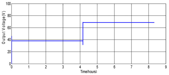
Figure 15.
Output voltage vs. time to variable duty cycle.
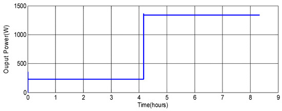
Figure 16.
Power vs. time to variable duty cycle.
These responses show the efficiency of proposed DC/DC converter.
The high performance of this average model of the DC/DC converter is due to the least squares method used. The simulated data was analysed to calculate the efficiency of converter, which was calculated based on energy extracted by converter.
• Scenario 3:
R = 10 Ω, both unbalanced duty cycle and photovoltaic voltage during a day. These variables are illustrated in Figure 17.
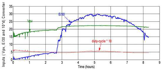
Figure 17.
Inputs (d, Vpv, and irradiation) vs. time.
In this case the tracing of the maximum power point is introduced into system.
The decrease output power of system illustrate in Figure 18 is caused by the variable duty cycle between 0.52 and 0.65.
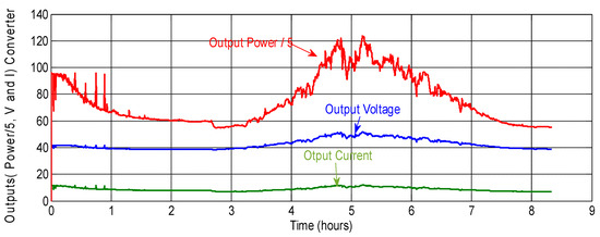
Figure 18.
Outputs (current, V0, and power) vs. time.
7. Regulation and Simulation Results
7.1. Regulation Parameters and Transfer Function
In 1942, Ziegler and Nichols proposed two heuristic approaches based on their experience and some simulations to adjust the parameters of the regulators P (proportional), PI (proportional-integral), and PID (proportional-integral-derivative) [11,12,13]. The first method requires the recording of the index response in an open loop, while the second requires bringing the looped system up to its limit of stability.
The control parameters of the system are determined in Figure 19:
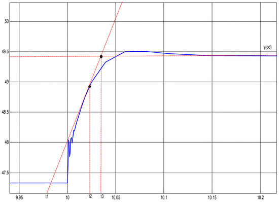
Figure 19.
Indicial response of the process.
The parameters are controlled by Ziegler-Nichols’s method (see Figure 19).
The T1, T2, and T3 instances illustrated in the following figure allow us to determine the following:
- The retard appears at L = t1
- The apparent time constant is T = t2 − t1
- The slope of the tangent at the point of inflection is Static gain k0 is the ratio between the asymptotic value y(∞) and the amplitude applied as input.
- The coefficients of the chosen regulator can then be calculated using Table 3.
Table 3. Parameters of the PID (proportional-integral-derivative) controller.
Hence, kp = 0.0015 and ki = 0.33.
In a closed loop, the control voltage follows the schema depicted below (Figure 20). The output of the PI controller compensates for the duty cycle to maintain the voltage at a desired reference value.
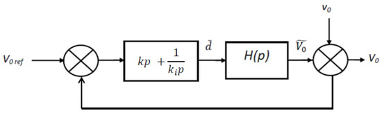
Figure 20.
Control voltage.
Finally, the transfer function is:
7.2. Simulation Result
The parameters of the system used for simulation are shown in Table 4.
Table 4.
The parameters of the DC/DC converter and load.
In the following, we present the simulation result of the photovoltaic electric-vehicle system in a closed loop under constant charge (R = 50 Ω) and varying reference voltages (V0ref) from 60 V to 70 V.
Figure 21 shows the response of the proposed control structure for the change of the photovoltaic voltage.
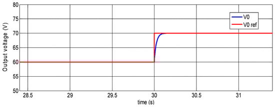
Figure 21.
Closed loop system response.
8. Conclusions
In this paper, the basic idea was to achieve the optimization of the transfer of power between the GPV and load under unbalanced irradiation throughout a day.
To achieve this aim:
- A controller was designed to stabilize the photovoltaic solar-vehicle system and then guarantee a zero-control deviation based on the application of the PID controller.
- A numerical method (MPPT) was used to track the maximal power that is generated by the photovoltaic array.
The properties of the proposed control’s structure were verified by simulation, as well as by the MPPT method.
The main advantage of the proposed control structure, employing a PID controller and the MPPT method, is the strong robustness over a wide range of parameter changes.
The obtained simulation results demonstrated that the proposed method is effective for DC/DC bus tension control and the optimization of the transfer of power from the GPV to load. Indeed, it is applicable in other types of nonlinear similar structure systems, and therefore it is possible to assume its wide application in industrial practice.
In this work, an average model of the interlaced DC/DC boost converter was studies and implemented.
This study takes into account only the parasitic resistance of the MOSFET, and the diode was developed.
Author Contributions
This paper is the results of the work of all authors, A.J., C.B.B., W.N. and F.B. They implemented the control strategies and performed experimental and simulation results. All authors contributed in bibliographical research, analysis and discussions of the results.
Acknowledgments
This work was partly supported by the Tunisian Ministry of Higher Education and Research under Laboratory of Computer Science for Industrial Systems (LISI), INSAT, University of Carthage, and Research Laboratory in Information and Communication Technologies & Electrical Engineering (LaTICE), ENSIT, University of Tunis.
Conflicts of Interest
The authors declare no conflict of interest.
Appendix
References
- Amari, M.; Ghouili, J.; Bacha, F. New High-Frequency Unidirectional DC-DC Converter for Fuel-Cell Electrical. IEEE Trans. Ind. Electron. 2012, 59, 1451–1458. [Google Scholar] [CrossRef]
- Amari, M.; Khelifi, J.I.; Bacha, F. Average Model of Dual Active Bridge Interfacing Ultra-capacitor in Electrical Vehicle. In Proceedings of the Fifth International Renewable Energy Congress (IREC), Hammamet, Tunisia, 25–27 March 2014. [Google Scholar]
- Güneşer, M.T.; Erdil, E.; Cernat, M.; Öztürk, T. Improving the Energy Management of a Solar Electric Vehicle. Adv. Electr. Comput. Eng. 2015, 15, 53–62. [Google Scholar] [CrossRef]
- Sarkar, T.; Sharma, M.; Gawre, S.K. A Generalized Approach to Design the Electrical Power System of a Solar Electric Vehicle. In Proceedings of the Electronics and Computer Science, Bhopal, India, 1–2 March 2014; pp. 1–6. [Google Scholar] [CrossRef]
- Sarkar, M.N.I. Effect of various model parameters on solar photovoltaic cell simulation: A SPICE analysis. Renew. Wind Water Sol. 2016, 3, 13. [Google Scholar] [CrossRef]
- Jendoubi, A.; Fnaiech, N.; Bacha, F. Advanced Numerical MPPT Approach for an Energy-storage Photovoltaic System under Unbalanced Climatic Conditions. Int. J. Control Theory Appl. 2017, 10, 51–68. [Google Scholar]
- Jendoubi, A.; Fnaiech, N.; Bacha, F. New Multivariate Polynomial Interpolation-Based MPPT. Applied to Battery Storage Photovoltaic System. Int. J. Control Energy Electr. Eng.-CEEE 2017, 4, 1–6. [Google Scholar]
- Araneo, R.; Grasselli, U.; Celozzi, S. Assessment of a practical model to estimate the cell temperature of a photovoltaic module. Int. J. Energy Environ. Eng. 2014, 5, 2. [Google Scholar] [CrossRef]
- Chao, R.-M.; Ko, S.-H.; Lin, H.-K.; Wang, I.-K. Evaluation of a Distributed Photovoltaic System in Grid-Connected and Standalone Applications by Different MPPT Algorithms. Energies 2018, 11, 1484. [Google Scholar] [CrossRef]
- Espinoza Trejo, D.R.; Bárcenas, E.; Hernández Díez, J.E.; Bossio, G.; Espinosa Pérez, G. Open- and Short-Circuit Fault Identification for a Boost dc/dc Converter in PV MPPT Systems. Energies 2018, 11, 616. [Google Scholar] [CrossRef]
- Kiyak, E.; Gol, G. A comparison of fuzzy logic and PID controller for a single-axis solar tracking system. Renew. Wind Water Sol. 2016, 3, 7. [Google Scholar] [CrossRef]
- Peretz, Y. A Randomized Algorithm for Optimal PID Controllers. Algorithms 2018, 11, 81. [Google Scholar] [CrossRef]
- Dalen, C.; Di Ruscio, D. Performance Optimal PI controller Tuning Based on Integrating Plus Time Delay Models. Algorithms 2018, 11, 86. [Google Scholar] [CrossRef]


© 2018 by the authors. Licensee MDPI, Basel, Switzerland. This article is an open access article distributed under the terms and conditions of the Creative Commons Attribution (CC BY) license (http://creativecommons.org/licenses/by/4.0/).