Optimization of Antenna Array Deployment for Partial Discharge Localization in Substations by Hybrid Particle Swarm Optimization and Genetic Algorithm Method

Abstract

A radio frequency antenna array was adopted to localize partial discharge (PD) sources in an entire substation. The deployment of an antenna array is a significant factor affecting the localization accuracy, and the array needs to be carefully selected. In this work, a hybrid method of particle swarm optimization (PSO) and a genetic algorithm (GA) is proposed to optimize the array deployment. A direction-of-arrival (DOA) estimation algorithm applicable to arbitrary array configurations is firstly presented. The Cramér-Rao lower bound (CRLB) was employed to evaluate the localization accuracy of different arrays, and two objective functions characterizing the estimation errors of coordinates and the DOA are proposed. With the goal of minimizing the objective functions, the array deployments for the coordinate and DOA localizations were optimized by using the hybrid PSO/GA algorithm. Using the developed method, optimal antenna configurations for different constraint areas, aspect ratios, and numbers of sensors were investigated. The results indicate that the optimal deployments for coordinate and DOA estimations are different; specifically speaking, superior DOA performance is achieved when all antennas are placed on the outer boundary of the constraint area while part of the antennas in the optimal coordinate array are placed in the middle position.

1. Introduction

Dielectric breakdown originating from insulating defects in high-voltage electrical equipment is a main cause of power supply interruption. Various techniques have been developed to discover potential defects prior to insulation failure. Owing to high sensitivity and abundant information, partial discharge (PD) measurement is extensively applied to assess the insulation conditions of power equipment. Online PD monitoring instruments have been mounted on some crucial equipment, such as gas-insulated substations (GISs) and transformers [1,2,3]. In consideration of installation cost, power utility companies are not willing to adopt such techniques for other equipment such as breakers, potentials, and current transformers. In order to detect the PD of all equipment in an entire air-insulated substation, a radio-frequency (RF) antenna array-based sensing system was developed [4,5]. The adopted detection bandwidth is generally in the frequency of 200 MHz to 2 GHz [6,7,8]. By utilizing the differences in the time of arrival (TOA) or amplitude of signals in the array elements, the equipment containing PD sources can be localized. Various kinds of localization techniques, including the received signal strength (RSS), time difference of arrival (TDOA), and TOA, have been exploited. Among these methods, the TDOA is the most widely used for its high accuracy [4,5,6,7,8,9].

The inaccuracy of the TDOA localization technique mainly comes from the TD estimation error and antenna positioning error; the antenna positioning error can be reduced by precise geometric measurement. Moreover, the localization accuracy is also greatly affected by the deployment of the antenna array, which needs to be carefully chosen. Initially, a Y-shaped array was adopted to find the discharge sources on the distribution line [10,11]. After that, Moore et al. compared the performance of rectangular and Y arrays, and they found that the rectangular array was superior to the Y array in terms of location accuracy [4]. The localization accuracies of rectangular, Y, and trapezoid arrays were investigated by numerical simulations and experiments in [12,13], and the results indicated that a trapezoid array presents a higher accuracy and lower dispersion. As we have demonstrated in previous research, the optimal array is dependent on the size, aspect ratio, and shape of the constraint area; however, only the single case is considered in most of the existing research, and the derived conclusions lack generality [14]. Passive localization is also a continuous theme of other research fields, such as radar, sonar, and wireless communication, and the Cramér-Rao lower bound (CRLB) is usually employed to characterize the localization accuracy [15,16,17,18]. For linear arrays, Hahn derived the sensor placements with the objective of minimizing the CRLB, and he found that the optimal performance was achieved when half of sensors were placed in the middle and one-quarter of the sensors each were on the left and right ends [15]. Under a circular constraint area, Ho et al. derived the optimum geometries for estimating the range and bearing by a systematic approach [16]. By using CRLB calculation, simulation of the root-mean-square error (RMSE), and experiments, we also investigated the influence of the size, aspect ratio, and shape of antenna arrays confined in a rectangular area [14]. From the above analysis, it could be found that optimal array deployments were different for different cases, and most of the optimization techniques suffered from one or more restrictions, such as the size, shape, and aspect ratio of the constraint area. For this reason, a general method for the optimization of sensor deployment was needed.

In this work, a hybrid method of particle swarm optimization (PSO) and a genetic algorithm (GA) is proposed to derive the optimum deployment for coordinate and direction-of-arrival (DOA) estimations. In Section 2, the theories for estimating the coordinates and DOA of PD sources are briefly described. The objective functions based on the CRLB are proposed in Section 3. After that, the idea and flowchart of the hybrid PSO/GA algorithm are presented in Section 4. Finally, in Section 5, the optimum geometries under different aspect ratios, constraint areas, and numbers of antennas, as obtained with the proposed algorithm, and the results, as confirmed with RMSE simulations, are presented.

2. Localization of PD Sources in Substation

By using the TDOAs between antennas, PD source localization can be achieved in two different ways, namely, coordinate and DOA estimations. In the first case, the coordinates of sources can be directly solved from the TDOA equations. Additionally, the DOA of incident electromagnetic (EM) waves, that is, the azimuth and elevation angles, can be estimated with TDOAs between antennas; then the locations of PD sources are calculated as the intersection points of DOAs estimated in several positions. In this section, the basic theories and estimation algorithms for coordinate and DOA localizations are shortly summarized, which provides a theoretical basis and localization algorithms for the following content. The optimization of the array deployments for both coordinate and DOA estimations is also described in the following sections. The corresponding objective functions and optimization results are illustrated in Section 3 and Section 5, respectively.

2.1. Coordinate Estimation

To accurately estimate the coordinates of PD sources, the antenna array needs to be placed on a broad space with a length greater than 4 m and is generally mounted on the roof of the control room [4,14]. Under these circumstances, the distance between the antenna array and discharge sources, that is, the distance between the equipment area and control room, is relatively large. For the relatively short height of power equipment compared to the large horizontal distance, the substation is usually regarded as a two-dimensional space. Moreover, because the obstacles have a minor effect on the signal propagation, the substation is considered as a line-of-sight (LOS) environment in almost all published research; thus the TDOA equations are expressed as follows [4,5,6,8,9,10,11,12]:

$$d_{ij}=\sqrt{{\left(x-x_i\right)}^2+{\left(y-y_i\right)}^2}-\sqrt{{\left(x-x_j\right)}^2+{\left(y-y_j\right)}^2}=c\left(t_{ij}+e_{ij}\right),$$

(1)

where s = [x, y] is the coordinates of the PD sources; s_i= [x_i, y_i] is the position of the ith antenna for i = 1, 2, …, M, where M is the number of antennas; t_ij is the TDOA between the ith and jth antennas; t_ij = t_i – t_j, where t_i is the TOA of the ith antenna; e_ij is the error of t_ij; and c is the propagation speed of EM waves.

TDOA equations are highly nonlinear formulas, and it is difficult or even impossible to derive the analytic solution. For this reason, various numerical algorithms such as the Newton-Raphson method, PSO, and grid-by-grid searching are adopted. Moreover, with the help of the least-squares (LS) estimation method, several closed-form solutions such as those of the Chan algorithm, spherical-interpolation, two-step weighted LS, and squared range-difference LS can be introduced [19,20,21]. The summarization of various algorithms can be found in [22].

2.2. DOA Estimation

A DOA estimation method is presented in [23] to determine the azimuth and elevation angles of a PD source with four antennas, but the algorithm requires that the straight lines passing through two pairs of antennas should be perpendicular. Because high-accuracy DOA estimation can be obtained even for a sensor array of small size, antennas are generally mounted on a movable platform to detect PDs in inspection roads of the substation. In this case, the antenna array is close to the power equipment and its height cannot be ignored; the substation cannot be considered as a two-dimensional space, and azimuth and elevation angles are all estimated. To estimate DOAs for arbitrary arrays, a novel LS algorithm is introduced [24]. Figure 1 depicts the positions of PD sources and antennas; Equations (2)–(4) can be derived according to the geometric relations:

$$\frac{S}{c}u\left(\phi ,\theta \right)=T+\epsilon ,$$

(2)

$$S=\left[\begin{array}{c}{s}_2-s_1\\ ⋮\\ s_M-s_1\\ s_3-s_2\\ ⋮\\ s_M-s_2\\ ⋮\\ s_M-s_{M-1}\end{array}\right]T=\left[\begin{array}{c}{t}_{12}\\ ⋮\\ t_{1M}\\ t_{23}\\ ⋮\\ t_{2M}\\ ⋮\\ t_{M-1,M}\end{array}\right],$$

(3)

$$u\left(\phi ,\theta \right)={\left[u_x,u_y,u_z\right]}^T={\left[\cos \left(\phi \right)\cos \left(\theta \right),\sin \left(\phi \right)\cos \left(\theta \right),\sin \left(\theta \right)\right]}^T,$$

(4)

where s_i= [x_i, y_i, z_i] is the coordinate of the ith antenna; φ and θ are the azimuth and elevation, respectively; u(φ, θ) is the DOA vector; T is the estimated TDOA array; and ε represents the measurement noise of the TDOA. By employing the LS technique, u(φ, θ) can be calculated as

$$u\left(\phi ,\theta \right)=c{\left(S^{T}S\right)}^{-1}{S}^{T}T.$$

(5)

Then the azimuth and elevation are expressed as

$$\begin{array}{c}\phi ={\tan }^{-1}\left(u_y/u_x\right)\hfill \\ \theta ={\tan }^{-1}\left(u_z/\sqrt{u_x^2+u_y^2}\right)\hfill \end{array}.$$

(6)

3. Objective Functions for Array Deployment Optimization

For a LOS environment, many works have demonstrated that the estimated TDOAs conform to a Gaussian distribution and that the CRLB can be used to describe the best achievable mean-square error (MSE), which is algorithm-independent. Here, the CRLB is adopted to characterize the localization accuracy of the antenna array [15,16,17,18]. Two objective functions are proposed from the CRLB of the coordinate and DOA estimations.

3.1. Objective Function for Coordinate Estimation

The CRLB is defined as the inverse of the Fisher information matrix (FIM). Ho and Hahn derived the computational formulas of the FIM for coordinate estimation in two-dimensional (2D) space as follows [14,16]:

$$\mathrm{FIM}\left(s=\left(r,\phi \right)\right)=\left[\begin{array}{l}XY\\ YZ\end{array}\right],$$

(7)

where s is expressed with polar coordinates and the other components are calculated from

$$\begin{array}{l}X=\frac{2}{{\sigma }_t^{2}M}{\left(\frac{1}{2c{r}^2}\right)}^2{X}^{\prime }\\ Y=\frac{2}{{\sigma }_t^{2}M}\left(\frac{-1}{2c^2{r}^2}\right)Y^{\prime }\\ Z=\frac{2}{{\sigma }_t^{2}M}\left(\frac{1}{c^2}\right)Z^{\prime }\end{array},$$

(8)

$$\begin{array}{l}{X}^{\prime }=\left\{M{\displaystyle \sum _{i=1}^M{l}_i^4{\sin }^4\left(\phi -{\mathbf{\varphi }}_i\right)}-{\left[{\displaystyle \sum _{i=1}^M{l}_i^2{\sin }^2\left(\phi -{\mathbf{\varphi }}_i\right)}\right]}^2\right\}\\ Y^{\prime }=\left\{M{\displaystyle \sum _{i=1}^M{l}_i^3{\sin }^3\left(\phi -{\mathbf{\varphi }}_i\right)}-\left[{\displaystyle \sum _{i=1}^M{l}_i^2{\sin }^2\left(\phi -{\mathbf{\varphi }}_i\right)}\right]\left[{\displaystyle \sum _{i=1}^M{l}_i\sin \left(\phi -{\mathbf{\varphi }}_i\right)}\right]\right\}\\ Z^{\prime }=\left\{M{\displaystyle \sum _{i=1}^M{l}_i^2{\sin }^2\left(\phi -{\mathbf{\varphi }}_i\right)}-{\left[{\displaystyle \sum _{i=1}^M{l}_i\sin \left(\phi -{\mathbf{\varphi }}_i\right)}\right]}^2\right\}\end{array},$$

(9)

where r and φ are the range and azimuth of PD sources, respectively; σ_t is the standard deviation of the TDOA error, which characterizes the noise level; M is the number of antennas; the $X^{\prime }, Y^{\prime }$, and $Z^{\prime }$ are terms related to the antenna arrangement; and l_i and ϕ_i are the range and azimuth of the ith antenna.

Then the CRLB for coordinate estimation can be expressed as

$$\mathrm{CRLB}\left(r\right)=\frac{Z}{XZ-Y^2}=2c^2{\sigma }_t^2{r}^4\cdot \frac{M{Z}^{\prime }}{X^{\prime }{Z}^{\prime }-{Y^{\prime }}^2},$$

(10)

which is composed of two separate terms. The first term is a function of c², ${\sigma }_t^2$, and r⁴. The second term depends on the antenna array deployment via $X^{\prime }, Y^{\prime }$, and $Z^{\prime }$. As the CRLB represents the variance of estimation, the standard deviation form, that is, e_r = $\sqrt{\mathrm{CRLB}(r)}$, is adopted. As can be seen from Equation (10), the CRLB is linearly related to ${\sigma }_t^2$ and r⁴, and the array deployment affects the CRLB via the second term. As a result, the second term was mainly investigated in the deployment optimization, and r and σ_t were set as fixed typical values. Owing to the linear relationship between CRLB and r⁴ or ${\sigma }_t^2$, the optimization results are applicable to other r and σ_t values, that is, other ranges and noise levels. Because the second term is dependent on the azimuth φ, the relation curve of e_r – φ was adopted to evaluate the localization performance of different deployments.

As the CRLB varied with the azimuth φ of the PD sources in some cases, the optimal deployment represents the configuration with the overall best performance considering all azimuths. More specifically, the objective was to minimize the CRLB in an azimuth range that was as wide as possible. Two types of deployments were taken as examples to illustrate the objective function. In the first case, a square array with a size of 4 m × 4 m and one element placed on each corner was employed. In the second deployment, the positions of antennas were arbitrarily selected, the coordinates of which were (−1.6, 1.2), (0.5, 0.8), (1.7, −1.5), and (−1.8, 0.3). The e_r curves of the two deployments are shown in Figure 2. In the calculation, r was set as 10 m, which is a typical distance between the PD sources and the array center in the substation, and σ_t was set as 0.2 ns according to our previous experiments [22]. The objective function J is defined as

$$J=J_1+J_2+J_3,$$

(11)

$$\begin{array}{c}{J}_1={\phi |}_{e_r>e_t}\hfill \\ J_2={\displaystyle \int \min \left\{e_r\left(\phi \right),e_t\right\}\mathrm{d}\phi }\hfill \\ J_3=\min \left\{e_r\left(\phi \right)\right\}\hfill \end{array}.$$

(12)

The function J is composed of three terms, which are described as follows. As can be seen from Figure 2, e_r was not uniform with respect to the azimuth angles in some cases, particularly for arrays with a number of antennas of less than four and with an irregular distribution, but was relatively high under some azimuths. For this reason, a threshold error e_t was defined to represent the maximum acceptable localization error, and J₁ is the range of azimuths (in radians) with e_r greater than e_t. Here, e_t was set as 20% of r. J₂ represents the area of the shadow part as shown in Figure 2, whose upper boundary was composed with minor points of e_r and e_t under all azimuths. J₂ characterizes the overall value of e_r under all azimuths. J₃ is the minimum value of the e_r curve. As can be seen from Figure 2b, the minimum e_r was higher than e_t for some poor array distributions, and J₁ and J₂ were equal to constant values of 2π and 4π, respectively. Under these circumstances, the objective was to minimize J₃, that is, the minimum value of e_r. J₁ and J₂ become relevant when the minimum e_r is less than e_t. Briefly, the objective function firstly tries to reduce the minimum e_r and then minimizes the overall localization error under all azimuths, which are represented by J₁ and J₂.

3.2. Objective Function for DOA Estimation

The CRLB for DOA estimation has been derived in some literature works and is shown as follows [17,18]:

$$\mathrm{CRLB}\left(\mathbf{\varphi }\right)={\left[G\left(B,\mathbf{\varphi }\right)\cdot P\right]}^{-1},$$

(13)

$$P=\frac{2M}{c^2{\sigma }_t^2},$$

(14)

$$G\left(B,\mathbf{\varphi }\right)={\frac{\partial u\left(\mathbf{\varphi }\right)}{\partial \mathbf{\varphi }}}^{T}B\frac{\partial u\left(\mathbf{\varphi }\right)}{\partial \mathbf{\varphi }},$$

(15)

$$B=\frac{1}{M}{\displaystyle \sum _{i=1}^M{\left(s_i-s_c\right)}^T\left(s_i-s_c\right)},$$

(16)

$$s_c=\frac{1}{M}{\displaystyle \sum _{i=1}^M{s}_i},$$

(17)

$$\mathbf{\varphi }={\left[\phi ,\theta \right]}^T.$$

(18)

The physical meanings of all parameters are illustrated in the former sections. Similarly to e_r, the standard derivation forms of CRLB(φ) and CRLB(θ) were employed here and are defined as e_φ and e_θ, respectively. The e_φ and e_θ forms are also composed of two separated terms, the former that is dependent on c² and ${\sigma }_t^2$ and the latter that is dependent on the array deployment. The DOA accuracy is irrelevant to the range r of the PD sources. For this reason, ${\sigma }_t^2$ was set as a fixed value, similarly to coordinate estimation, and the array deployment was optimized by minimizing the DOA error in all azimuths and over a wide range of elevations.

Taking a square array with a size of 1 m × 1 m and one element placed on each corner as an example, the distributions of e_φ and e_θ were computed as is shown in Figure 3. The input parameters were the same as for the e_r calculation. Because the antennas were distributed uniformly in the horizontal plane, e_φ and e_θ were constant for all azimuths. The e_φ value increased with elevation, while the e_θ value decreased when the elevation increased. Moreover, it could be found that the e_φ and e_θ values were satisfactory even when the array size was just 1 m × 1 m. From the above, a simple objective function was adopted:

$$J=\mathrm{mean}\left\{{e_{\phi }|}_{-180°<\phi \le 180°,10°\le \theta \le 70°}+{e_{\theta }|}_{-180°<\phi \le 180°,10°\le \theta \le 70°}\right\},$$

(19)

where “mean” indicates the calculation of the average value of the summation of e_φ and e_θ for φ in the range of −180° to 180° and θ of 10° to 70°. Considering the height of the power equipment, elevations of less than 10° and of more than 70° were ignored.

3.3. Constraints

The constraints for array optimization are dependent on the shape and size of the constraint area. In this work, two kinds of constraint areas, rectangular and circular, were investigated. For a rectangular constraint with a size of a × b, the chromosome in the GA/particle in PSO is coded with Cartesian coordinates, that is, X = [x₁, x₂, …, x_M, y₁, y₂, …, y_M], and is constrained by the following equations:

$$\begin{array}{c}-a/2\le x_i\le a/2\hfill \\ -b/2\le y_i\le b/2\hfill \end{array}.$$

(20)

For a circular constraint with radius r_c, the chromosome/particle is coded with polar coordinates, X = [r₁, r₂, …, r_M, φ₁, φ₂, …, φ_M], and is constrained by

$$\begin{array}{c}0\le r\le r_c\hfill \\ -180°\le \phi \le 180°\hfill \end{array}.$$

(21)

In the computation of the fitness value, the chromosome/particle is transformed into the corresponding coordinate system needed for the objective function.

4. Hybrid PSO/GA Algorithm for Optimization of Array Deployment

As can be seen from the objective functions of the coordinate and DOA estimations, the array deployment is optimized to achieve the best overall performance considering all azimuths. To reach this target, objective functions with complex expressions are proposed, which cannot be written with analytical formulas. Moreover, the objective functions present local optimums. As a result, a global searching algorithm, such as PSO/GA, is needed. In this section, the concepts of PSO and the GA are firstly recalled. Then, the proposed array deployment optimization method, based on the hybrid PSO/GA algorithm, is introduced.

4.1. Genetic Algorithm and Particle Swarm Optimization

The GA is formulated by simulating the biological genetic evolution process. The GA generally starts with a randomly generated initial population, which is composed of a certain number of individuals or chromosomes. The surviving probability of each individual is evaluated by means of a fitness function. Fit individuals are selected to perform the crossover operation to produce a new generation. After that, a mutation operator is applied to the population to decrease the possibility of becoming stuck in a local optimum [25].

The PSO is inspired by social and cognitive behavior and was proposed by Kennedy and Eberhart [26]. A swarm consists of a group of particles/individuals, which update their locations to obtain the optimal solution by a self-adaptive velocity. The velocity is dependent on the previous velocity of the particle, the current location, the personal best position representing private thinking, and the global best representing the collaboration among particles. Therefore, the particles have a tendency to move toward better solutions over the searching process.

4.2. Hybrid PSO/GA Algorithm

It was found that PSO can memorize the global and personal bests and affect the motion of all particles, resulting in quick convergence [26]. However, it lacks crossover and mutation operators and is more easily stuck in a local optimum. For this reason, it was hoped that a better and quicker solution would be obtained by a hybrid of PSO and the GA. Here, two kinds of hybrid methods, namely, parallel and series, were employed; these have similar searching procedures, except for the individuals for the crossover and mutation operations. The flowchart of the parallel hybrid algorithm is shown in Figure 4. The solutions can be achieved by the following steps.

Step 1: Set up the values of input parameters, including the population size (here 2000), crossover rate (0.8), and mutation rate (0.2). Many test iterations were performed for different input parameters and constraints, and we found that the optimization process tended to fall into a local optimum in some cases. As a result, a large population size, crossover rate, and mutation rate are adopted to increase the diversity of individuals, which contributes to convergence to the global optimum. Because an overly large population size increases the computation time greatly, a moderate size of 2000 was adopted in this work. We found that the optimization process with these input parameters converged to the global optimum in almost all tests.

Step 2: Randomly generate the initial population with N particles. Calculate the objective function values of all particles, and then find and record the personal and global best solutions.

Step 3: Divide the population into two groups with sizes of N × P and N × (1 – P), and adopt PSO and GA in these two groups, respectively. P is the hybrid probability and was set as 0.3 in this work.

Step 4: PSO stage: The velocities and positions of particles are updated according to Equations (22)–(25):

$$v_i=w{v}_i+c_1\cdot r_1\cdot \left(P_i-X_i\right)+c_2\cdot r_2\cdot \left(P_g-X_i\right),$$

(22)

where

$$\begin{array}{c}w=\frac{2}{\phi -2+\sqrt{{\phi }^2-4\phi }}\hfill \\ \phi ={\phi }_1+{\phi }_2\hfill \\ c_1=w{\phi }_1\hfill \\ c_2=w{\phi }_2\hfill \end{array}.$$

(23)

Here, v_i is the current velocity of the ith particle; r₁ and r₂ are two pseudo-random numbers conforming to a uniform distribution in 0–1; X_i and P_i are the current position and personal best position, respectively; P_g is the global best position; and φ₁ and φ₂ are both set as 2.05. The flight velocity of the particles is limited by v_max, which is defined as

$$v_{\max }=\left(X_{\max }-X_{\min }\right)/10,$$

(24)

where X_max and X_min are the maximum and minimum constraints as described in Section 3.3.

The updated velocity is added to the current position to obtain the new position:

$$X_i=X_i+v_i.$$

(25)

After the positions of all particles are updated according to the above steps, the objective function values are computed, and then the new personal and global best solutions can be found.

Step 5: GA stage: A roulette-wheel strategy is adopted to select individuals for the crossover operation. The crossover of two individuals X₁ and X₂ is performed using

$$\begin{array}{l}{X}_1^{\mathrm{new}}=\omega \cdot X_1+\left(1-\omega \right)\cdot X_2\\ X_2^{\mathrm{new}}=\omega \cdot X_2+\left(1-\omega \right)\cdot X_1\end{array},$$

(26)

where X₁ and X₂ are parent individuals, $X_1^{\mathrm{new}}$ and $X_2^{\mathrm{new}}$ are child individuals, and $\omega$ is a random number in the range of 0–1. The particles for mutation are randomly selected, and the mutation operator is defined as

$$X^{\mathrm{new}}=X+\omega \cdot \left(X_{\max }-X_{\min }\right).$$

(27)

Step 6: The offspring populations generated by the PSO and GA stages are combined, and N particles with the best fitnesses are chosen as the elites to form the new population.

Step 7: Repeat steps 3–6 until the ending criterion is met.

The procedures of the series hybrid algorithm are similar to those of the parallel methods, except that the crossover is performed between the global and personal best solutions and mutation is only applied to the global best.

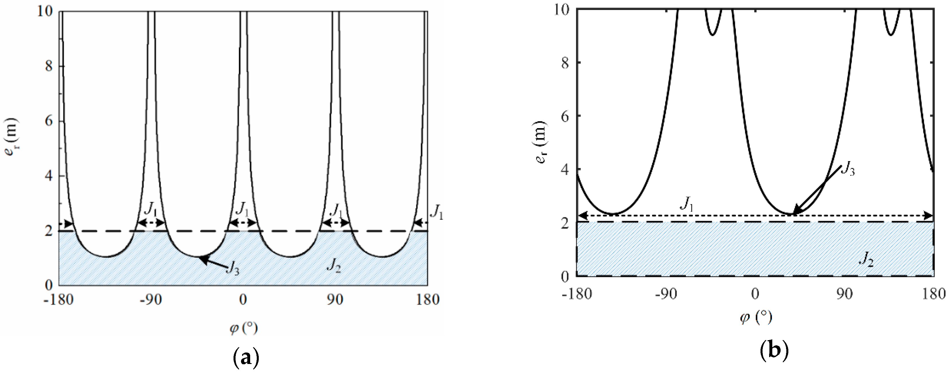
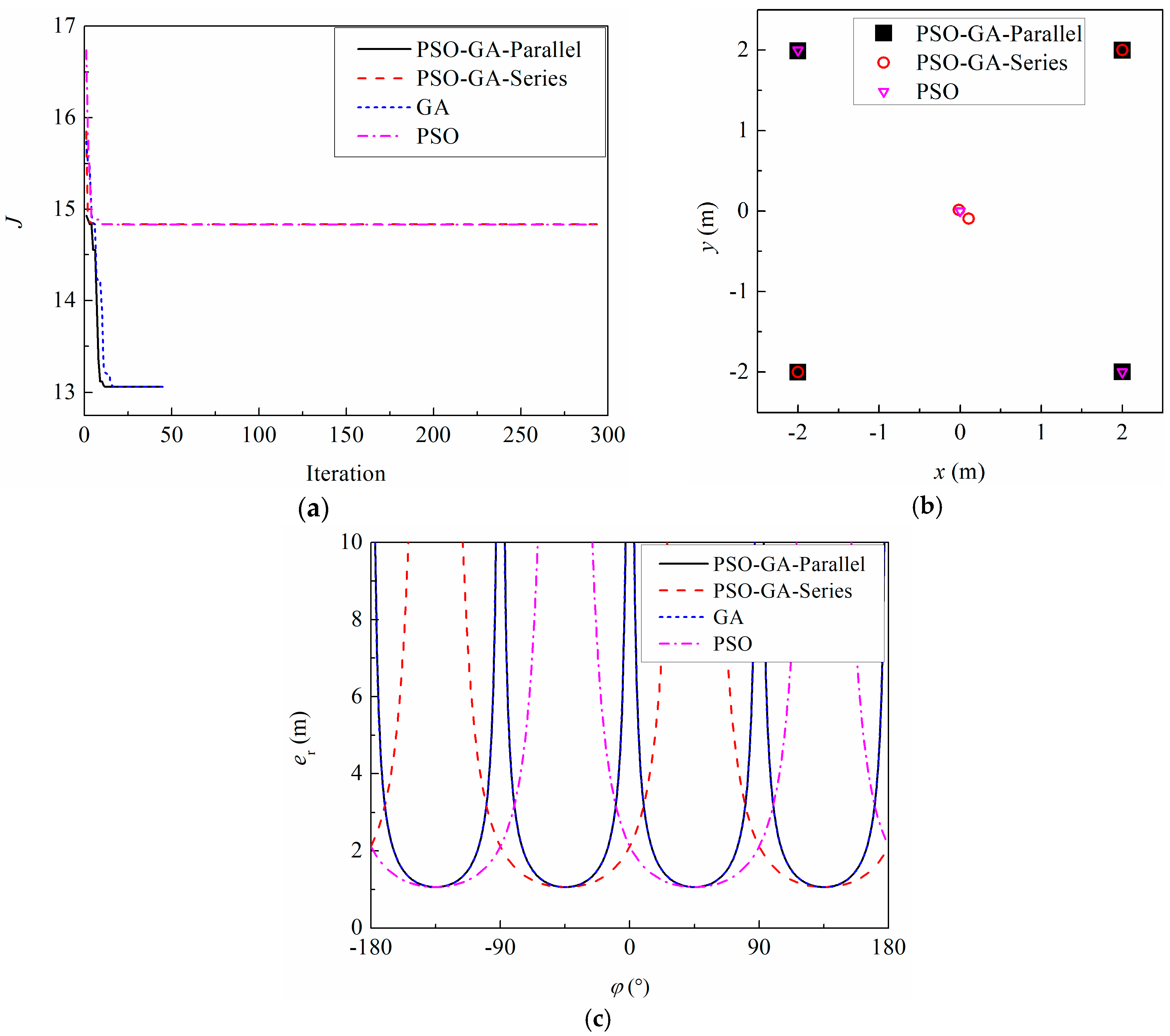
5. Results and Discussions

In this section, the performances of PSO, the GA, the parallel hybrid algorithm, and the series hybrid algorithm are firstly compared. Then, the array deployments for different aspect ratios, shapes of the constraint area, and numbers of antennas, as optimized with the proposed method, are described. For the coordinate estimation cases in Section 5.1 and Section 5.2, the optimization results gave the best overall array deployments for all PD positions with a fixed range (here 10 m) and an azimuth of −180° to 180°. For the DOA estimation cases in Section 5.3, the optimized arrays were overall optimal for PD locations within the azimuth range of −180° to 180° and elevation range of 10° to 70°. It should be noted that the proposed optimization method does not provide optimum array deployments for a specific PD position.

5.1. Comparison of Optimization Algorithms

A rectangular constraint area with a size of 4 m × 4 m was used to compare different optimization algorithms. Here, the comparison of the optimized array configurations for coordinate estimation is described. The results are shown in Figure 5, for which the optimized array of the GA was the same as that of the parallel hybrid method and is not presented in the figure. As can be seen, PSO and the series hybrid method converged quickly, but the final objective function value was 14.83, which was higher than 13.06 for the parallel hybrid and GA methods. The results indicate that PSO and the series hybrid method fall into a local optimum after 300 iterations, while the parallel and GA methods converge in less than 50 iterations. The obtained arrays for the parallel and GA methods were square, while those of the other two methods were linear, with two antennas placed in the middle. The minimum e_r values of the two types of arrays were identical, but the e_r curve of the square array had four valleys compared to two for the linear array. As described in Section 4, the optimization process tended to fall into a local optimum in some cases. The PSO method lacks crossover and mutation operations, which speed up the convergence process but make it easier to fall into a local optimum. This is the reason that PSO could not find the optimal array deployment in some cases. Despite GA being introduced into the series hybrid method, the crossover and mutation operations were only applied to personal and global bests, which sped up the convergence but could not effectively allow the local optimum to be avoided. Both the GA and parallel methods could find the global optimum, but the parallel hybrid algorithm converged faster than the GA. In contrast, the parallel hybrid method presented a superior convergence capability and was used in the following optimizations.

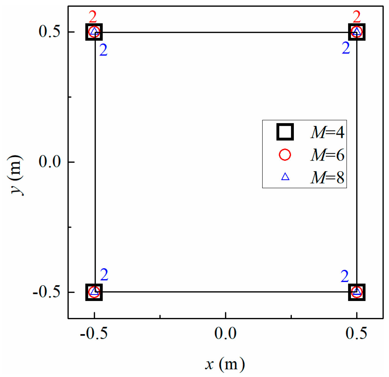
5.2. Array Deployment for Coordinate Estimation

The array deployments for rectangular constraint areas with sizes of 4 m × 4 m, 3 m × 4 m, 2 m × 4 m, and 1 m × 4 m, that is, aspect ratios of 1, 0.75, 0.5, and 0.25, were optimized with the parallel hybrid algorithm. The sensor array consisted of four antennas. Figure 6 depicts the optimized array deployments and CRLB curves. Because some of the elements overlapped, the number of overlapping sensors is indicated in the figure. For the areas of sizes 4 m × 4 m and 3 m × 4 m, the optimal shape was a rectangular array with one element placed on each corner of the constraint area, and the e_r curves had four bearings with high accuracy. When the constraint size was 2 m × 4 m or 1 m × 4 m, the optimal performance was achieved when two sensors were placed in the middle and two sensors were placed on the ends of a diagonal line. For a small aspect ratio, such as for the array size of 1 m × 4 m, the diamond shape presented almost the same accuracy as that of the linear array; hence the optimized deployment used was the diamond shape. The linear array only had two bearings with a minor e_r value, namely, the direction perpendicular to the sensor pair with the maximum distance. We also found that the threshold size for the change in the optimal shape from rectangular to linear was 2.6 m × 4 m.

As can be seen, the optimization results occasionally suggested placing two antennas at the same physical position. The reason for this is that the physical size of the antennas was not considered in the localization theories. In reality, two antennas cannot be placed at the same position. Because the size of antennas (generally with diameters of less than 20 cm) is far less than the distance between them, overlapping antennas can be placed around the optimized position within small distances, which causes negligible variation in the localization accuracy.

In the second case, the deployment for arrays with different numbers of sensors was optimized. A rectangular constraint area with a size of 4 m × 4 m was also adopted here. The optimization results and corresponding CRLB curves are shown in Figure 7. For M = 6, the optimal accuracy was obtained when one antenna was placed on each corner of the rectangular constraint and two antennas were placed at the center. Similarly, for the optimal shape for M = 8, one antenna was placed at each corner and four antennas were placed in the middle. As can be seen from the CRLB curves, the localization accuracy presented directivity when only four antennas were used, while the arrays with six or eight elements had almost the same errors under all azimuths. The e_r value was greatly reduced when the number of antennas was increased from four to six. The e_r value was further decreased when eight sensors were adopted.

To highlight the advantages of the proposed optimization algorithm, the localization accuracy of the optimized and reference arrays were compared. Here, eight antennas were adopted and two reference arrays (R1 and R2) with regular distributions were selected, as shown in Figure 8a. The CRLB and RMSE curves were compared, whereby the RMSE simulation was performed according to [14] and the setting parameters were the same as those in the CRLB calculation. The Chan algorithm was adopted to solve the PD coordinates in the RMSE simulation. From the results, it was found that the optimized array had the minimum error under all azimuths. R2 had two antennas in the middle and was closer to the optimized shape than R1; it showed better localization performance than R1. The comparison confirmed the effectiveness of the deployment optimization algorithm.

To further verify the optimization results, a higher noise level (σ_t was set as 0.4 ns) was adopted in the RMSE simulation. The RMSE results of the three arrays in Figure 8a were compared, as shown in Figure 9a. As can be seen, the optimized array still presented the minimum RMSE among the different arrays, which indicates that the optimization results are applicable to different noise levels. Despite that a substation is usually regarded as a LOS environment, the influence of obstacles such as insulation bodies is also discussed here. Under these circumstances, a non-line-of-sight (NLOS) environment is considered. In a NLOS environment, the TDOAs between some channels are contaminated by bias error. Assuming that t₃₁ and t₆₁ are contaminated by a bias error of 0.2 ns and that σ_t is set as 0.2 ns, the RMSE simulations were repeated, and the results are shown in Figure 9b. As can be seen, the optimized array gave the best localization performance among the three arrays. For this reason, it can be concluded that the deployment optimization method is applicable to NLOS environments to some extent.

In the case of the circular constraint area, the optimal deployments were different to those of the rectangular area. Here, a circular area with a radius of 2.83 m was considered, and the configurations for four, six, and eight antennas were optimized, as shown in Figure 10. For M = 4, the optimized shape had four antennas uniformly distributed on the circle. If six antennas were employed, superior performance was achieved when five sensors were uniformly placed on the circle and one was placed at the center. In the case of eight sensors, six antennas were uniformly placed on the circle and two antennas were placed at the center. Additionally, it can be seen that the CRLB values of the circular array were close to those of the rectangular array but showed more flat curves along different azimuths.

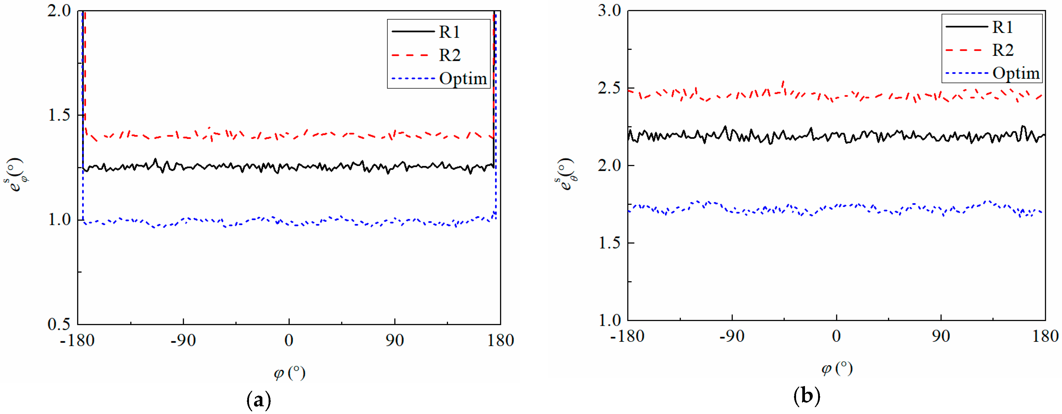
5.3. Array Deployment for DOA Estimation

In this section, the array deployment for DOA estimation was optimized. As described above, the DOA estimation accuracy was satisfied even when the array size was 1 m × 1 m, occupying a small space. To obtain a similar accuracy under different azimuths, uniform arrays are generally adopted. For this reason, the influence of the aspect ratio was not considered, and the array deployments for square and circular constraint areas were investigated. Figure 11 depicts the optimized array shapes for four, six, and eight antennas in a square area. Compared to the arrays for coordinate estimation shown in Figure 7, the optimal shapes for DOA estimation were different. Superior performance was achieved when all antennas were placed on the corners of the square area. For arrays with four or eight antennas, one or two elements are placed on each corner, respectively. If six antennas were adopted, two elements were placed on each upside corner and one element was placed on the other corners.

The optimized arrays and corresponding CRLB surfaces for the circular constraint are shown in Figure 12. It is evident that improved performance for DOA estimation was attained when all antennas were distributed on the circumference. The e_φ and e_θ values were identical under all azimuths and were reduced by increasing the number of antennas.

Two reference arrays were selected to compare their accuracies with that of the optimized configuration, as shown in Figure 13a. In one of the references, R2 was the optimal deployment for coordinate estimation. Figure 13b,c shows the CRLB surfaces of the azimuths and elevations for different configurations. Clearly, the optimized array outperformed R1 and R2 in terms of both the azimuth and elevation CRLB. The average errors of the azimuth and elevation angles under an elevation of 30° were simulated with similar procedures as for the RMSE, for which the method in Section 2.2 was employed to estimate the azimuth and elevation angles, and the results are shown in Figure 14. As can be seen, the optimized array presented the minimum error for both azimuth and elevation, which further confirms the accuracy of the proposed method.

6. Conclusions

This work aimed to improve the localization accuracy for PD sources in substations by means of optimizing the array deployment. By using the CRLB, objective functions evaluating the estimation accuracy of the PD coordinate and DOA are proposed. With the goal of minimizing the objective functions, the array deployments for coordinate and DOA localization are optimized by using a hybrid PSO/GA algorithm.

From the comparison of different types of optimization methods, it could be found that the parallel hybrid PSO/GA algorithm presented excellent global searching capability, and it was thus employed in this work. For a rectangular constraint area, the optimal array deployment for coordinate estimation is related to the aspect ratio; specifically speaking, a rectangular array with one antenna placed on each corner of the constraint area presents the optimal accuracy when the aspect ratio is higher than 0.65, and in other cases, the optimized shape is a linear array with two sensors placed in the middle and two sensors on the ends of the diagonal line. Moreover, the optimal deployments for coordinate and DOA estimations are different; more specifically, superior DOA performance is achieved when all antennas are placed on the outer boundary of the constraint area while part of the antennas in the optimal coordinate array are placed in the middle. The localization accuracy and homogeneity under different azimuths can be improved by adopting six or more sensors. The optimization results were confirmed by the RMSE simulations, which also verified the effectiveness of the proposed objective functions.

References

1. Schichler, U.; Koltunowicz, W.; Endo, F.; Feser, K.; Giboulet, A.; Girodet, A.; Tenbohlen, S. Risk assessment on defects in GIS based on PD diagnostics. IEEE Trans. Dielectr. Electr. Insul. 2013, 20, 2165–2172. [Google Scholar] [CrossRef]
2. Okabe, S.; Ueta, G.; Hama, H.; Ito, T.; Hikita, M.; Okubo, H. New aspects of UHF PD diagnostics on gas-insulated systems. IEEE Trans. Dielectr. Electr. Insul. 2014, 21, 2245–2258. [Google Scholar] [CrossRef]
3. Zheng, S.; Li, C.; Tang, Z.; Chang, W.; He, M. Location of PDs inside transformer windings using UHF methods. IEEE Trans. Dielectr. Electr. Insul. 2014, 21, 386–393. [Google Scholar] [CrossRef]
4. Moore, P.J.; Portugues, I.E.; Glover, I.A. Radiometric Location of Partial Discharge Sources on Energized High-Voltage Plant. IEEE Trans. Power Deliv. 2005, 20, 2264–2272. [Google Scholar] [CrossRef]
5. Portugues, I.E.; Moore, P.J.; Glover, I.A.; Johnstone, C.; McKosky, R.H.; Goff, M.B.; Van der Zel, L. RF-Based Partial Discharge Early Warning System for Air-Insulated Substations. IEEE Trans. Power Deliv. 2009, 24, 20–29. [Google Scholar] [CrossRef]
6. Hou, H.J.; Sheng, G.H.; Jiang, X.C. Localization Algorithm for the PD Source in Substation Based on L-Shaped Antenna Array Signal Processing. IEEE Trans. Power Deliv. 2015, 30, 472–479. [Google Scholar] [CrossRef]
7. Li, Z.; Luo, L.; Zhou, N.; Sheng, G.; Jiang, X. A Novel Partial Discharge Localization Method in Substation Based on a Wireless UHF Sensor Array. Sensors 2017, 17, 1909. [Google Scholar] [CrossRef] [PubMed]
8. Zhang, Q.; Li, C.; Zheng, S.; Yin, H.; Kan, Y.; Xiong, J. Remote detecting and locating partial discharge in bushings by using wideband RF antenna array. IEEE Trans. Dielectr. Electr. Insul. 2016, 23, 3575–3583. [Google Scholar] [CrossRef]
9. Li, P.; Zhou, W.; Yang, S.; Liu, Y.; Tian, Y.; Wang, Y. Method for partial discharge localisation in air-insulated substations. IET Sci. Meas. Technol. 2017, 11, 331–338. [Google Scholar] [CrossRef]
10. Tungkanawanich, A.; Kawasaki, Z.I.; Matsuura, K. Location of Multiple PD Sources on Distribution Lines by Measuring Emitted Pulse-Train Electromagnetic Waves. IEEJ Trans. Power Energy 2000, 120, 1431–1436. [Google Scholar] [CrossRef] [Green Version]
11. Tungkanawanich, A.; Kawasaki, Z.I.; Abe, J.; Matsuura, K. Location of partial discharge source on distribution line by measuring emitted pulse-train electromagnetic waves. In Proceedings of the 2000 IEEE Power Engineering Society Winter Meeting, Singapore, 23–27 January 2000; pp. 2453–2458. [Google Scholar]
12. Robles, G.; Fresno, J.M.; Sánchez-Fernández, M.; Martínez-Tarifa, J.M. Antenna Deployment for the Localization of Partial Discharges in Open-Air Substations. Sensors 2016, 16, 541. [Google Scholar] [CrossRef] [PubMed]
13. Robles, G.; Fresno, J.M.; Sánchez-Fernández, M.; Martínez-Tarifa, J.M. Antenna array layout for the localization of partial discharges in open-air substations. In Proceedings of the International Electronic Conference on Sensors Application, 15–30 November 2015; pp. 1–7. Available online: https://sciforum.net/conference/ecsa-2 (accessed on 10 July 2018).
14. Zhu, M.; Liu, Q.; Wang, Y.; Li, Y.; Deng, J.; Mu, H.-B.; Zhang, G.-J. Optimisation of Antenna Array Allocation for Partial Discharge Localisation in Air-Insulated Substation. IET Sci. Meas. Technol. 2017, 11, 967–975. [Google Scholar] [CrossRef]
15. Hahn, W.R.; Tretter, S.A. Optimum Processing for Delay-Vector Estimation in Passive Signal Arrays. IEEE Trans. Inform. Theory 1973, 19, 608–614. [Google Scholar] [CrossRef]
16. Ho, H.C.; Vicente, L.M. Sensor Allocation for Source Localization with Decoupled Range and Bearing Estimation. IEEE Trans. Signal Process. 2008, 56, 5773–5789. [Google Scholar] [CrossRef]
17. Baysal, Ü.; Moses, R.L. On the Geometry of Isotropic Arrays. IEEE Trans. Signal Process. 2003, 51, 1469–1478. [Google Scholar] [CrossRef]
18. Gazzah, H.; Marcos, S. Cramer-Rao Bounds for Antenna Array Design. IEEE Trans. Signal Process. 2006, 54, 336–345. [Google Scholar] [CrossRef]
19. Chan, Y.T.; Ho, K.C. A Simple and Efficient Estimator for Hyperbolic Location. IEEE Trans. Signal Process. 1994, 42, 1905–1915. [Google Scholar] [CrossRef]
20. Ho, H.C. Bias Reduction for an Explicit Solution of Source Localization Using TDOA. IEEE Trans. Signal Process. 2012, 60, 2101–2114. [Google Scholar] [CrossRef]
21. Li, X.; Deng, Z.D.; Rauchenstein, L.T.; Carlson, T.J. Contributed Review: Source-localization algorithms and applications using time of arrival and time difference of arrival measurements. Rev. Sci. Instrum. 2016, 87, 041502. [Google Scholar] [CrossRef] [PubMed] [Green Version]
22. Zhu, M.X.; Wang, Y.B.; Chang, D.G.; Zhang, G.J.; Tong, X.; Ruan, L. Quantitative Comparison of Partial Discharge Localization Algorithms Using Time Difference of Arrival Measurement in Substation. Int. J. Electr. Power Energy Syst. 2018, 104, 10–20. [Google Scholar] [CrossRef]
23. Tian, Y.; Tatematsu, A.; Tanabe, K.; Miyajima, K. Development of Locating System of Pulsed Electromagnetic Interference Source Based on Advanced TDOA Estimation Method. IEEE Trans. Electromagn. Compat. 2014, 56, 1326–1334. [Google Scholar] [CrossRef]
24. Cui, X.; Yu, K.; Lu, S. Evolutionary TDOA-Based Direction Finding Methods With 3-D Acoustic Array. IEEE Trans. Instrum. Meas. 2015, 64, 2347–2359. [Google Scholar]
25. Duan, H.; Luo, Q.; Ma, G.; Shi, Y. Hybrid Particle Swarm Optimization and Genetic Algorithm for Multi-UAV Formation Reconfiguration. IEEE Comput. Intell. Mag. 2013, 8, 16–27. [Google Scholar] [CrossRef]
26. Kuo, R.J.; Syu, Y.J.; Chen, Z.Y.; Tien, F.C. Integration of particle swarm optimization and genetic algorithm for dynamic clustering. Inf. Sci. 2012, 195, 124–140. [Google Scholar] [CrossRef]
Figure 1. Positions of partial discharge (PD) source and antennas.
Energies 11 01813 g001
Figure 2. Schematic diagram of objective function for coordinate estimation: (a) square array; (b) an arbitrary array.
Energies 11 01813 g002
Figure 3. Distributions of eφ and eθ for square array with size of 1 m × 1 m: (a) distribution of eφ; (b) distribution of eθ.
Energies 11 01813 g003
Figure 4. Flowchart of particle swarm optimization/genetic algorithm (PSO/GA) parallel algorithm.
Energies 11 01813 g004
Figure 5. Optimization results by using different algorithms: (a) evolution curve; (b) array deployment; (c) Cramér-Rao lower bound (CRLB) curve.
Energies 11 01813 g005
Figure 6. Optimization results of rectangular constraint area with different aspect ratios: (a) array deployment; (b) Cramér-Rao lower bound (CRLB) curve.
Energies 11 01813 g006
Figure 7. Optimization results for rectangular constraint areas with different numbers of antennas:(a) array deployment; (b) Cramér-Rao lower bound (CRLB) curve.
Energies 11 01813 g007
Figure 8. Comparison of optimized and reference arrays: (a) array deployment; (b) Cramér-Rao lower bound (CRLB) curve; (c) simulation of root-mean-square-error (RMSE).
Energies 11 01813 g008
Figure 9. Comparison of root-mean-square errors (RMSEs) of optimized and reference arrays under different time-difference-of-arrival (TDOA) characteristics: (a) σt was set as 0.4 ns; (b) t31 and t61 were contaminated by bias error of 0.2 ns.
Energies 11 01813 g009
Figure 10. Optimization results of circular constraint area with different numbers of antennas: (a) array deployment; (b) Cramér-Rao lower bound (CRLB) curve.
Energies 11 01813 g010
Figure 11. Optimized array deployments for direction-of-arrival (DOA) estimation in square constraint area.
Energies 11 01813 g011
Figure 12. Optimized array deployments for direction-of-arrival (DOA) estimation in circular constraint area: (a) array deployment; (b) Cramér-Rao lower bound (CRLB) of azimuth angle; (c) CRLB of elevation angle.
Energies 11 01813 g012
Figure 13. Comparison of optimized and reference arrays for direction-of-arrival (DOA) estimation: (a) array deployments; (b) Cramér-Rao lower bound (CRLB) of azimuth angle; (c) CRLB of elevation angle.
Energies 11 01813 g013
Figure 14. Comparison of average direction-of-arrival (DOA) errors for optimized and reference arrays: (a) average error of azimuth angle; (b) average error of elevation angle.
Energies 11 01813 g014