Investigation and Analysis of Attack Angle and Rear Flow Condition of Contra-Rotating Small Hydro-Turbine


Abstract
1. Introduction
2. Experimental Work
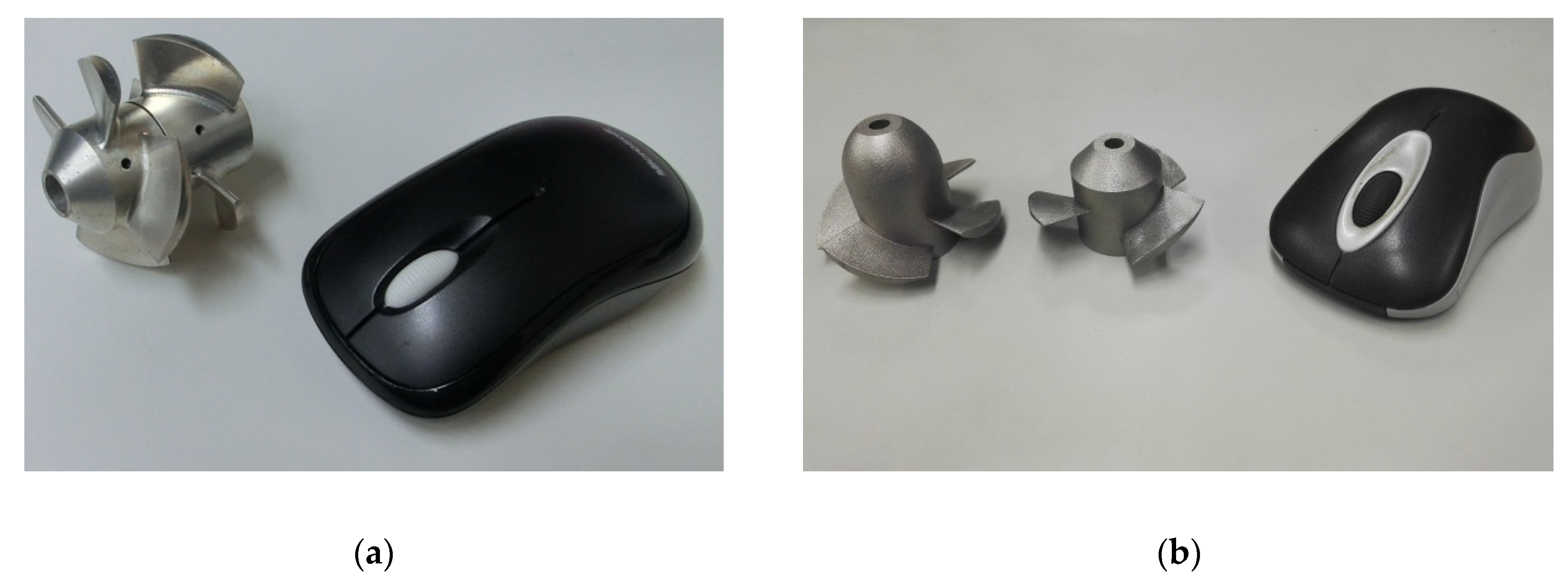
2.1. Basic Design Method of the Models
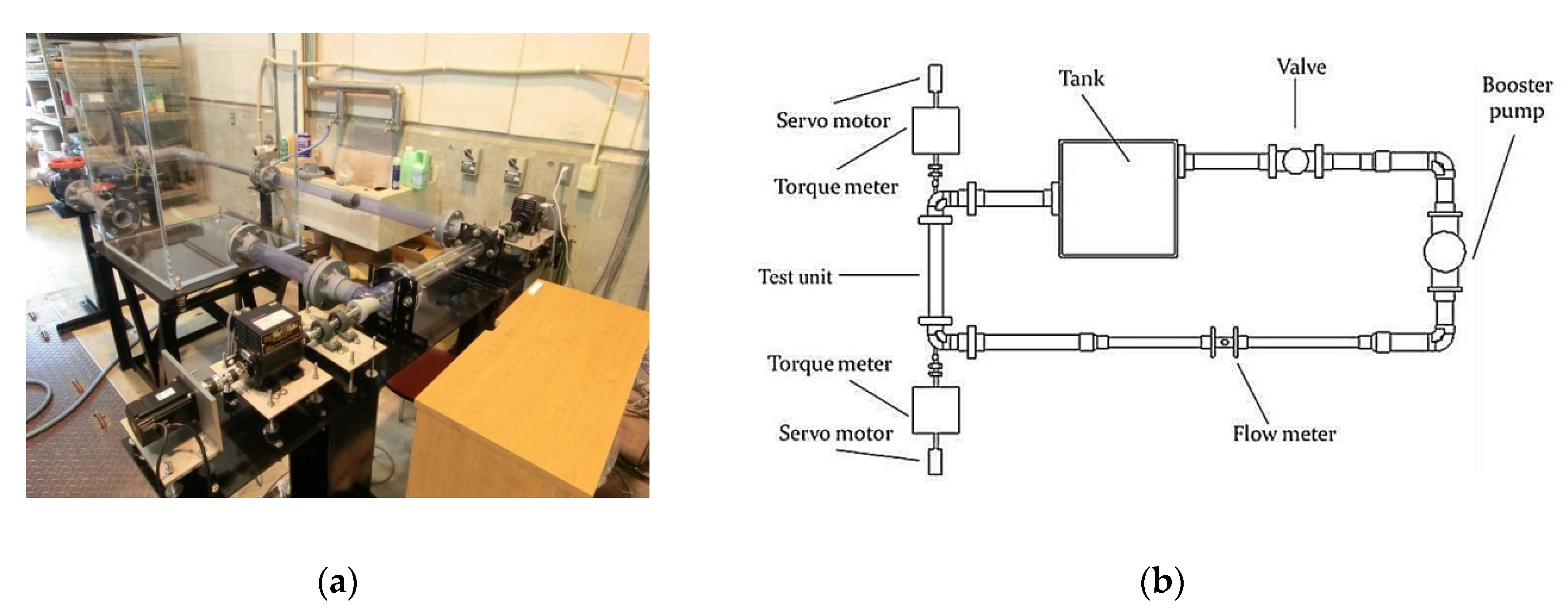
2.2. Experimental Apparatus and Method
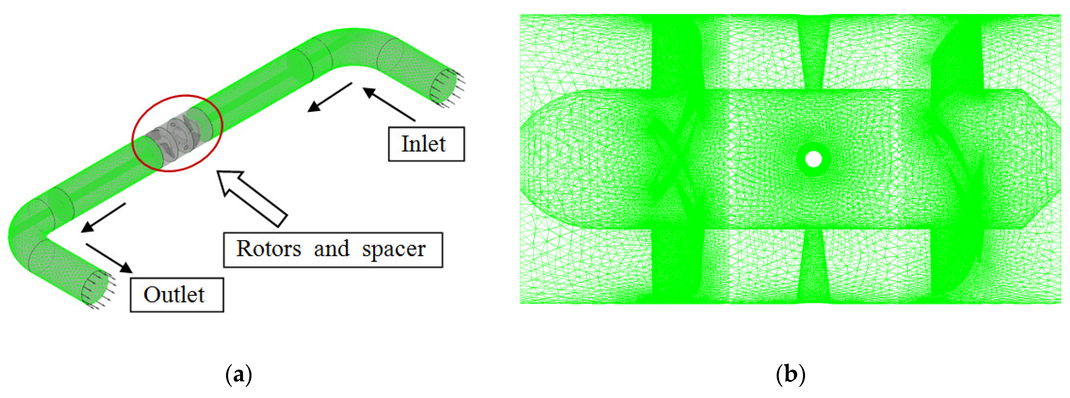
3. Numerical Analysis Conditions
4. Results and Discussions
4.1. Experimental Results of Original Model and New Model
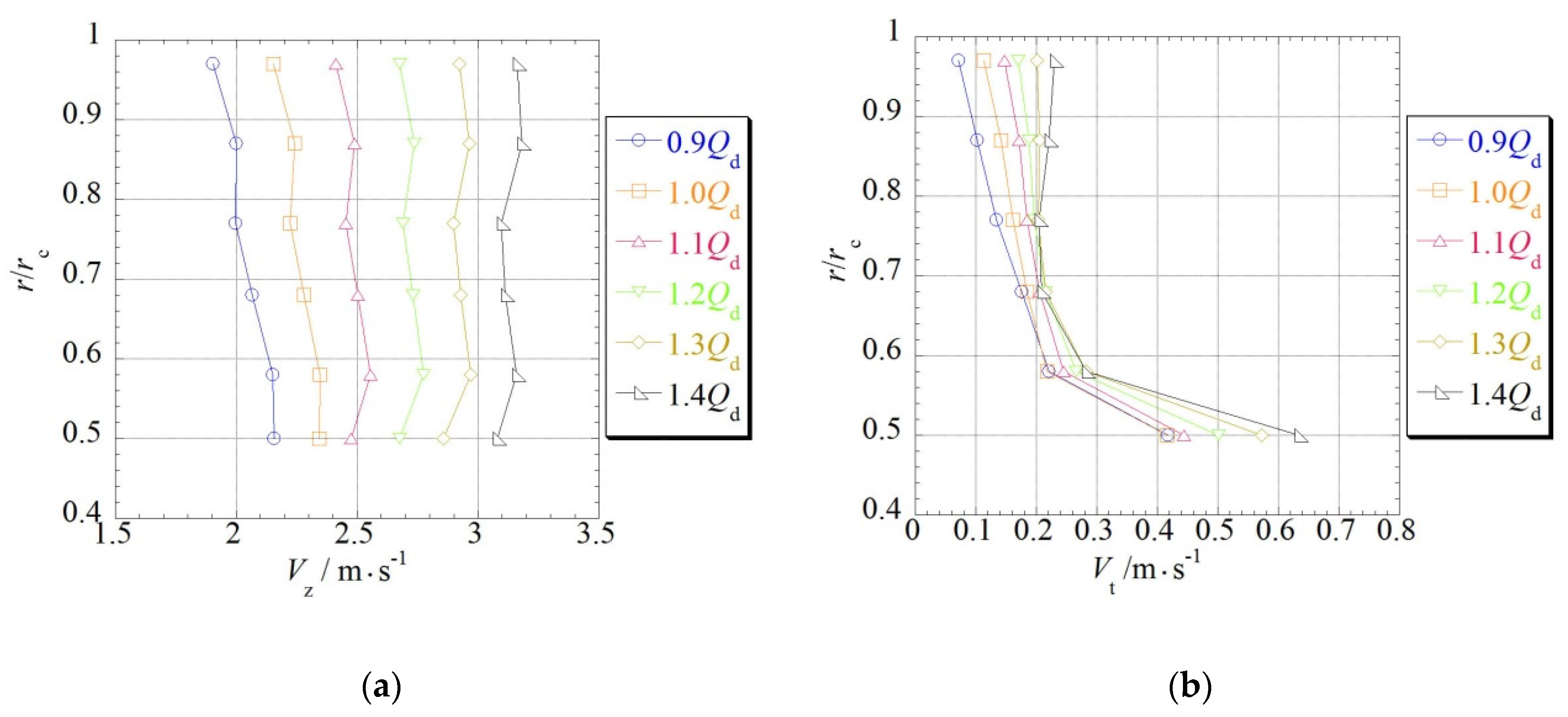
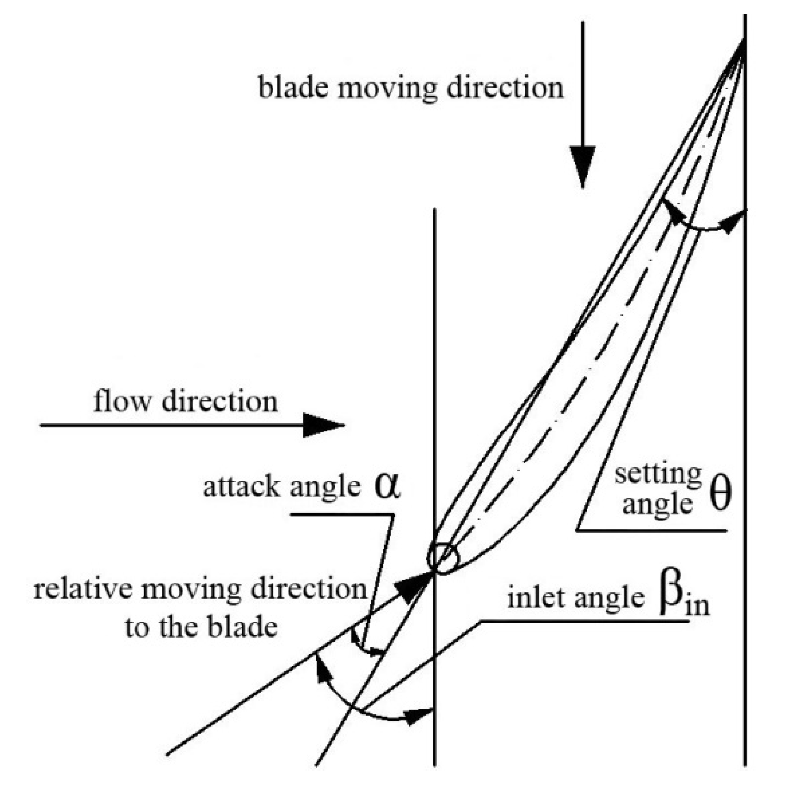
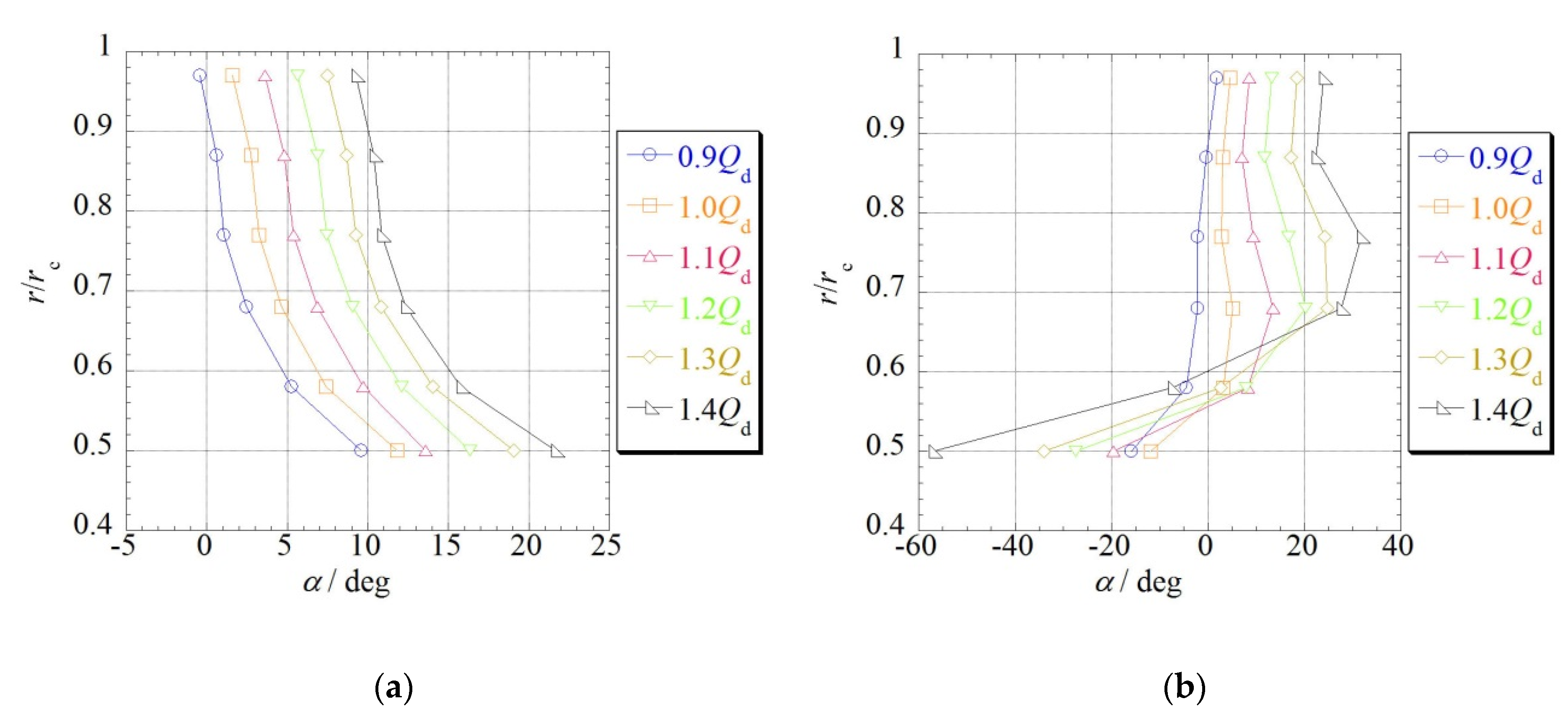
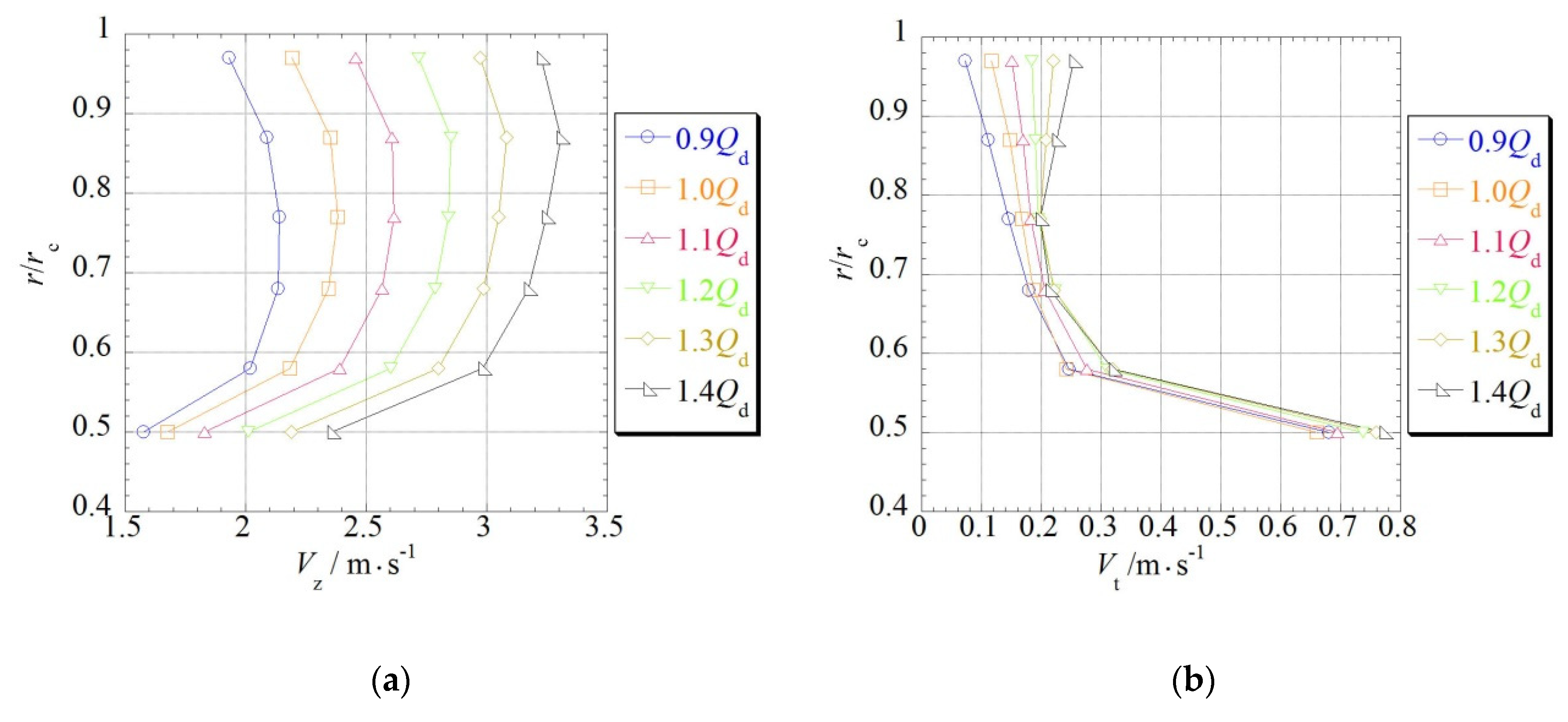
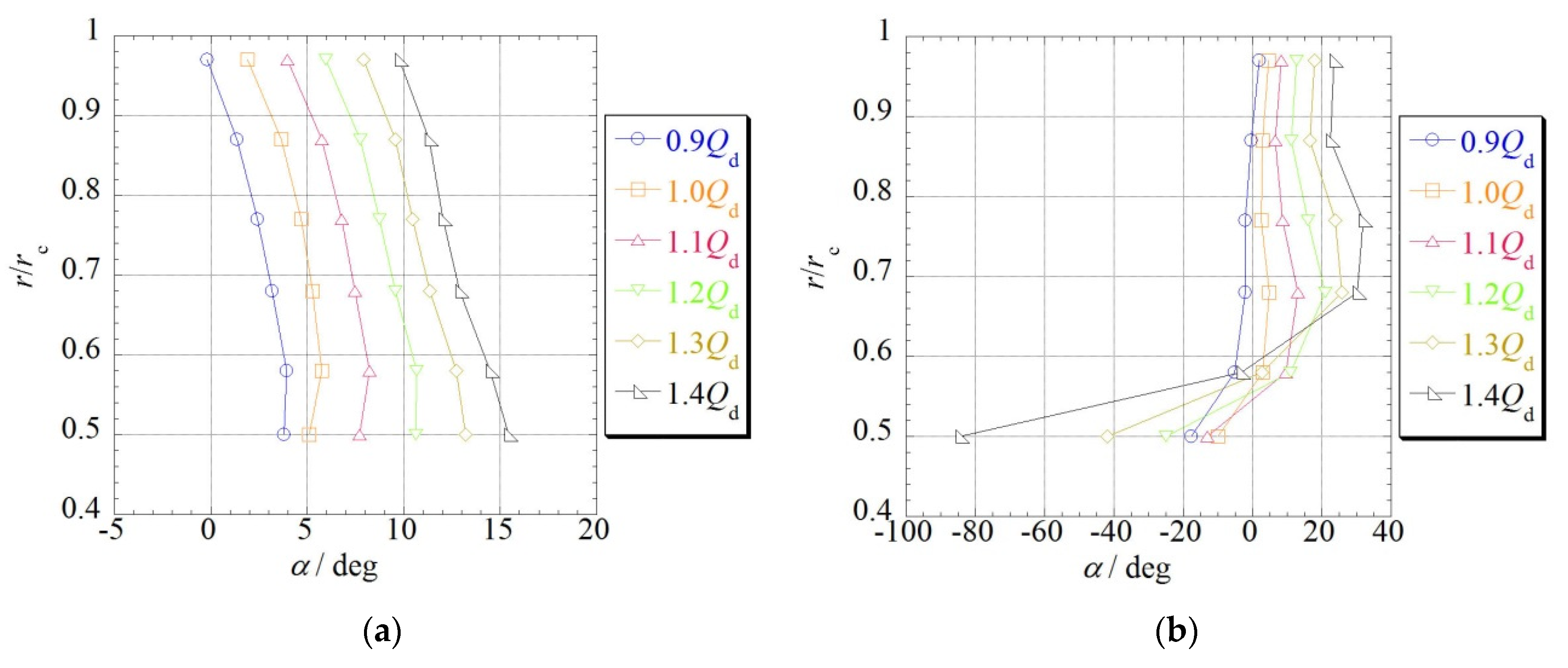
4.2. Investigation and Analysis on the Attack Angle
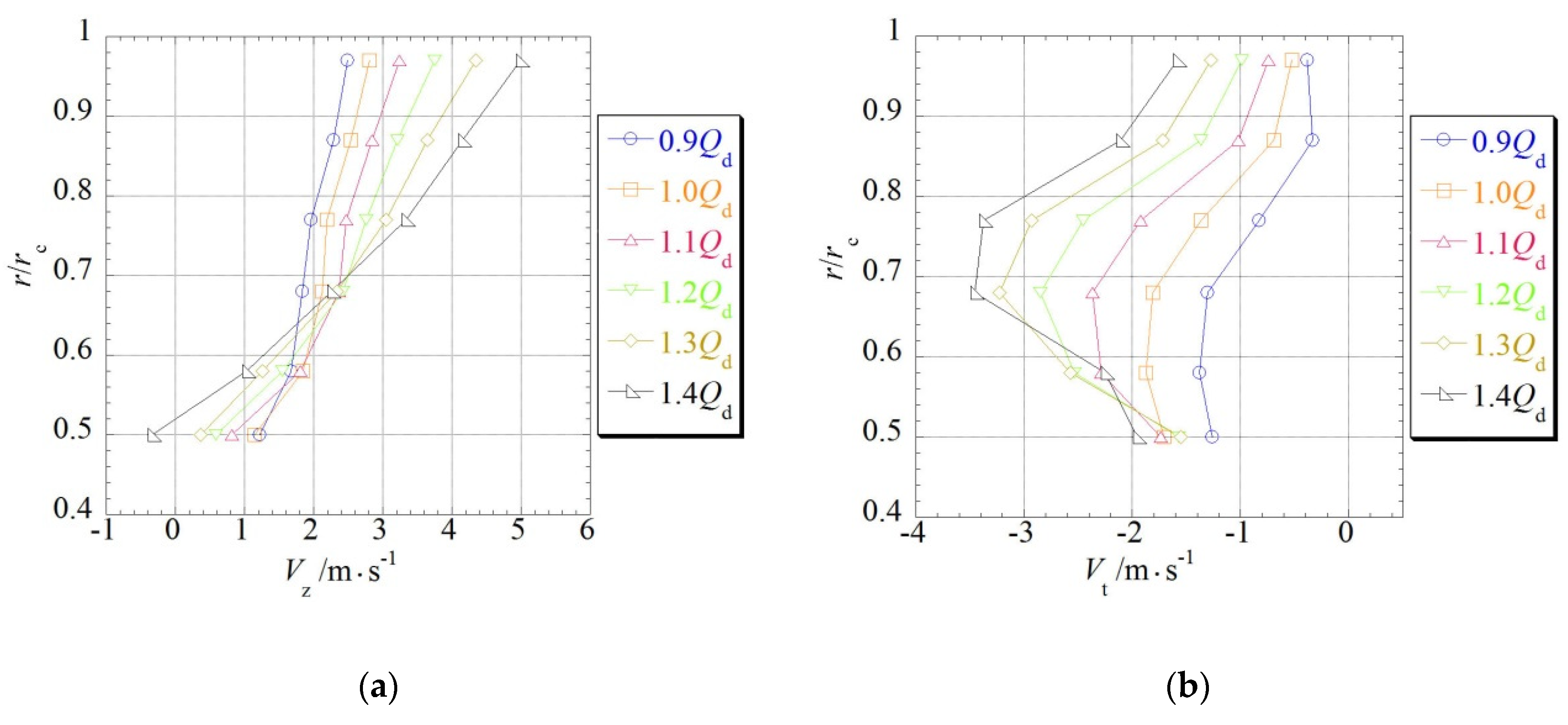
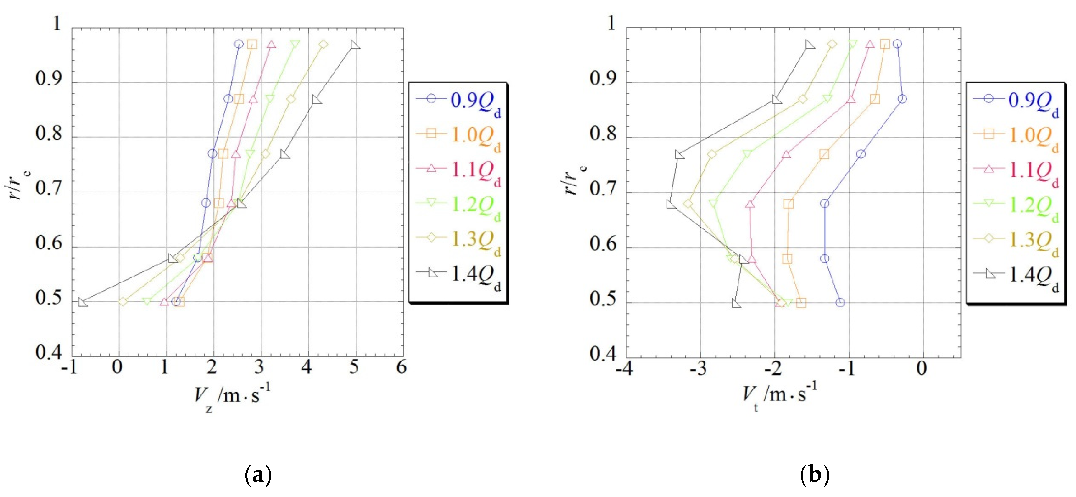
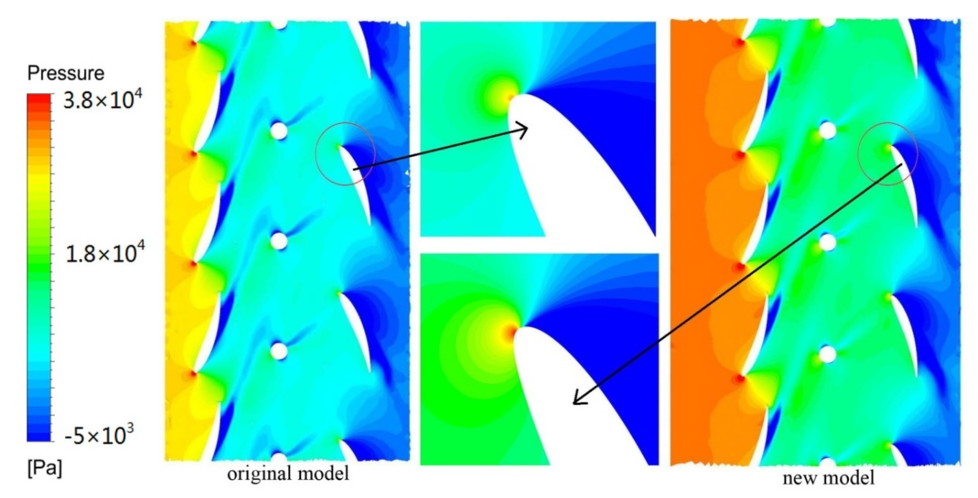
4.3. Investigation and Analysis on the Rear Flow Condition
5. Conclusions
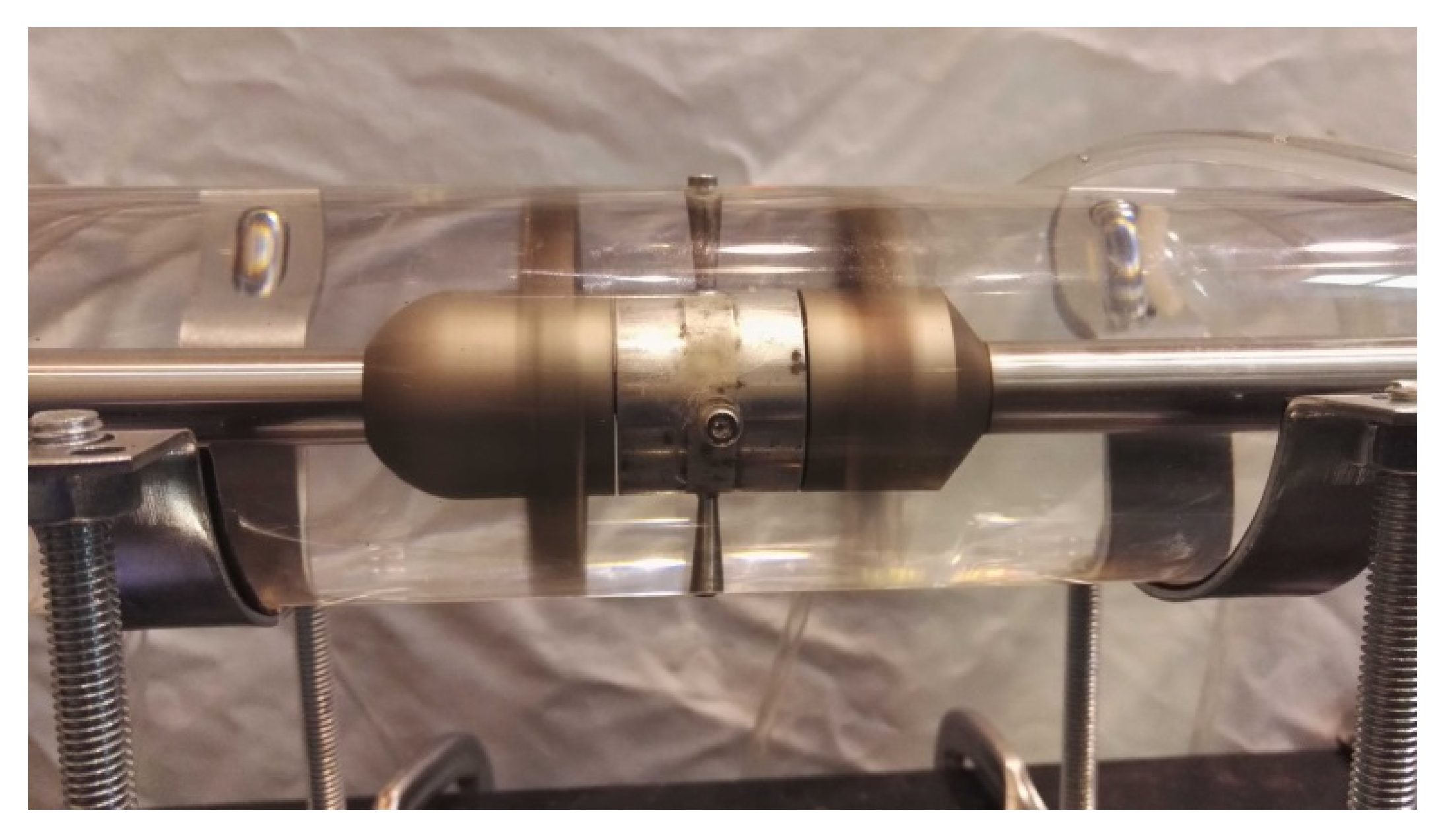
- The contra-rotating small hydro-turbine can be installed in water supplying systems in farmland settings, and remote rural areas can use the electrical power which is generated by this system. Besides, some support structures like guide vanes or fairwater can be used in this hydro-turbine. These support structures can help to improve the flow conditions. However, to make this contra-rotating small hydro-turbine as compact as possible, we did not adopt guide vanes and fairwater. We designed a spacer which includes four spokes to support the contra-rotating small hydro-turbine in the casing.
- The attack angle of the new model is smaller at the hub area. Therefore, the new front hub helps to decrease the front attack angle. This phenomenon proves that water can flow into the front blade more directly. It was for this reason that we changed the shape of the front hub; the attack angle demonstrates that we have achieved our goal. By means of changing the front attack angle, the rear flow condition is changed, and the performance was further improved.
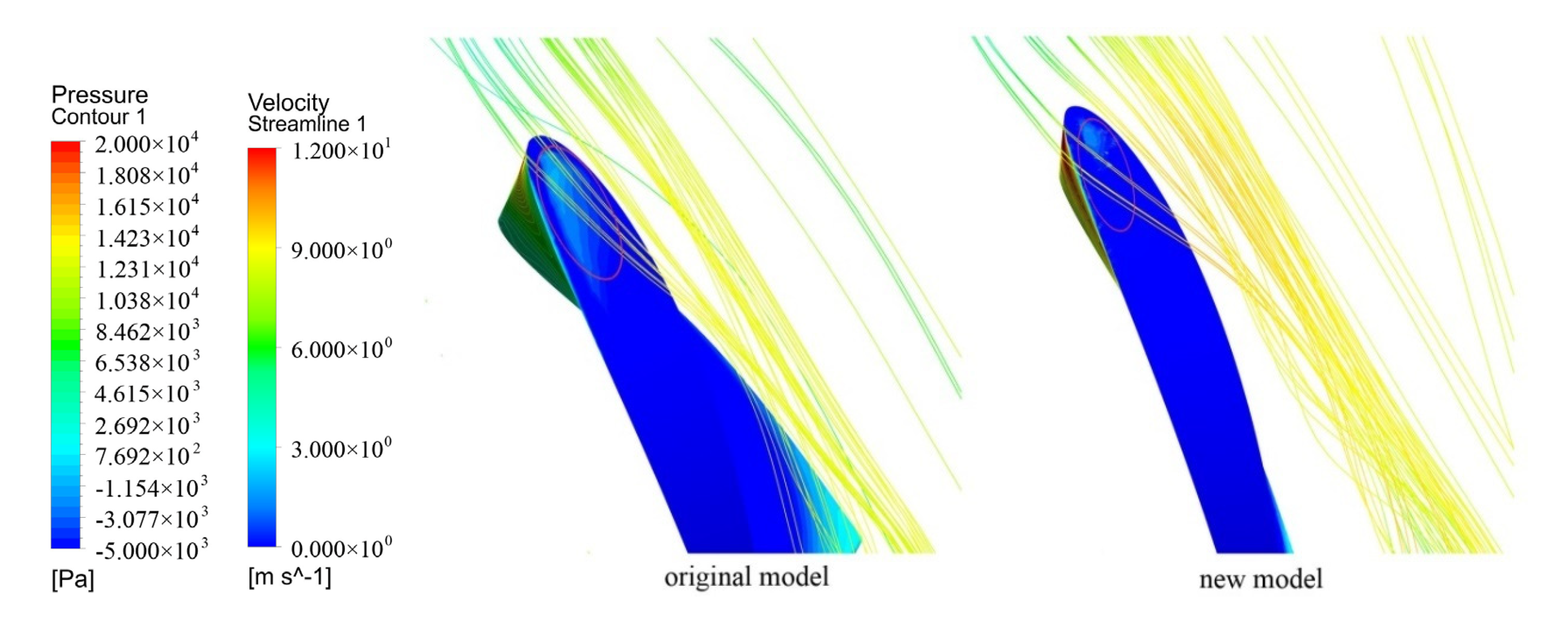
- Compared with the original model, the rear rotor’s stagnation point in new model is moved downward to the pressure surface of the rear blade. Because of this change to the stagnation point, the new model’s separation at the leading edge area is suppressed, while the original model’s separation at leading edge area is expanded in the cascade frontal line. Therefore, this change to the stagnation point helped to suppress separation at the leading edge area and improve the rear flow conditions.
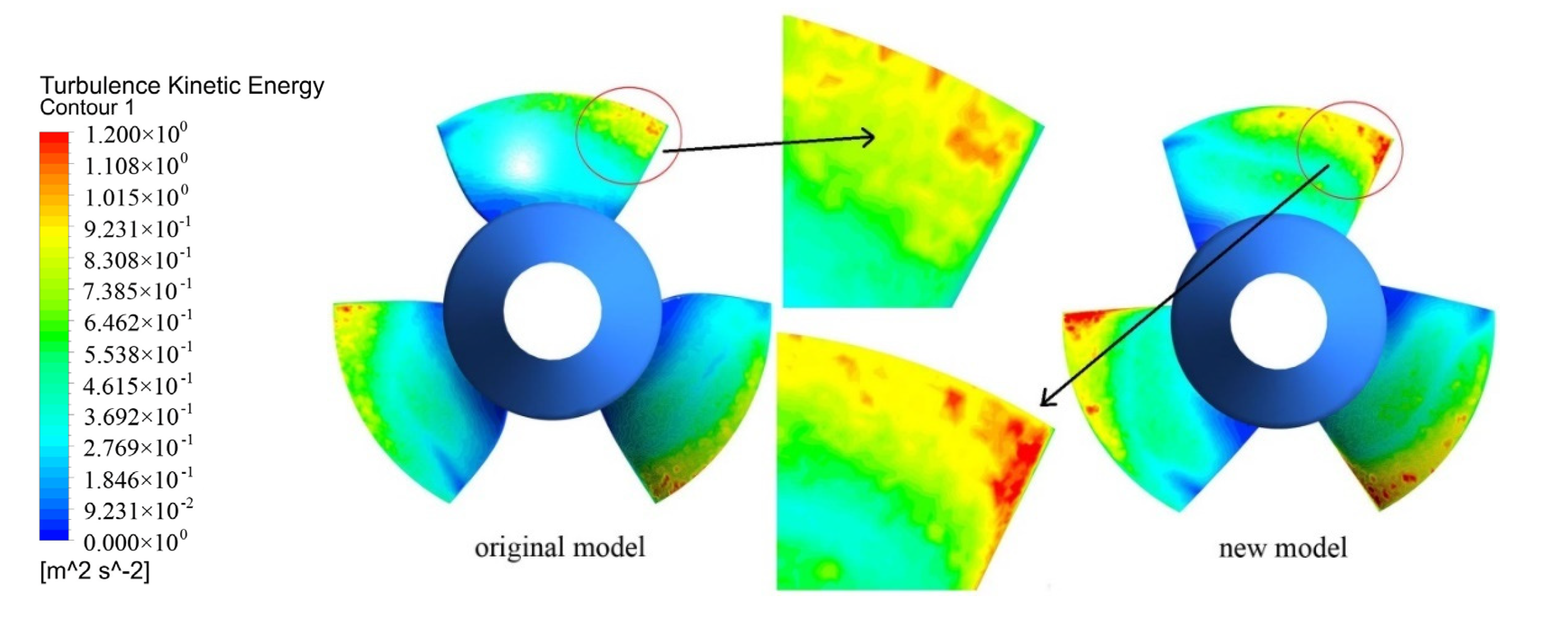
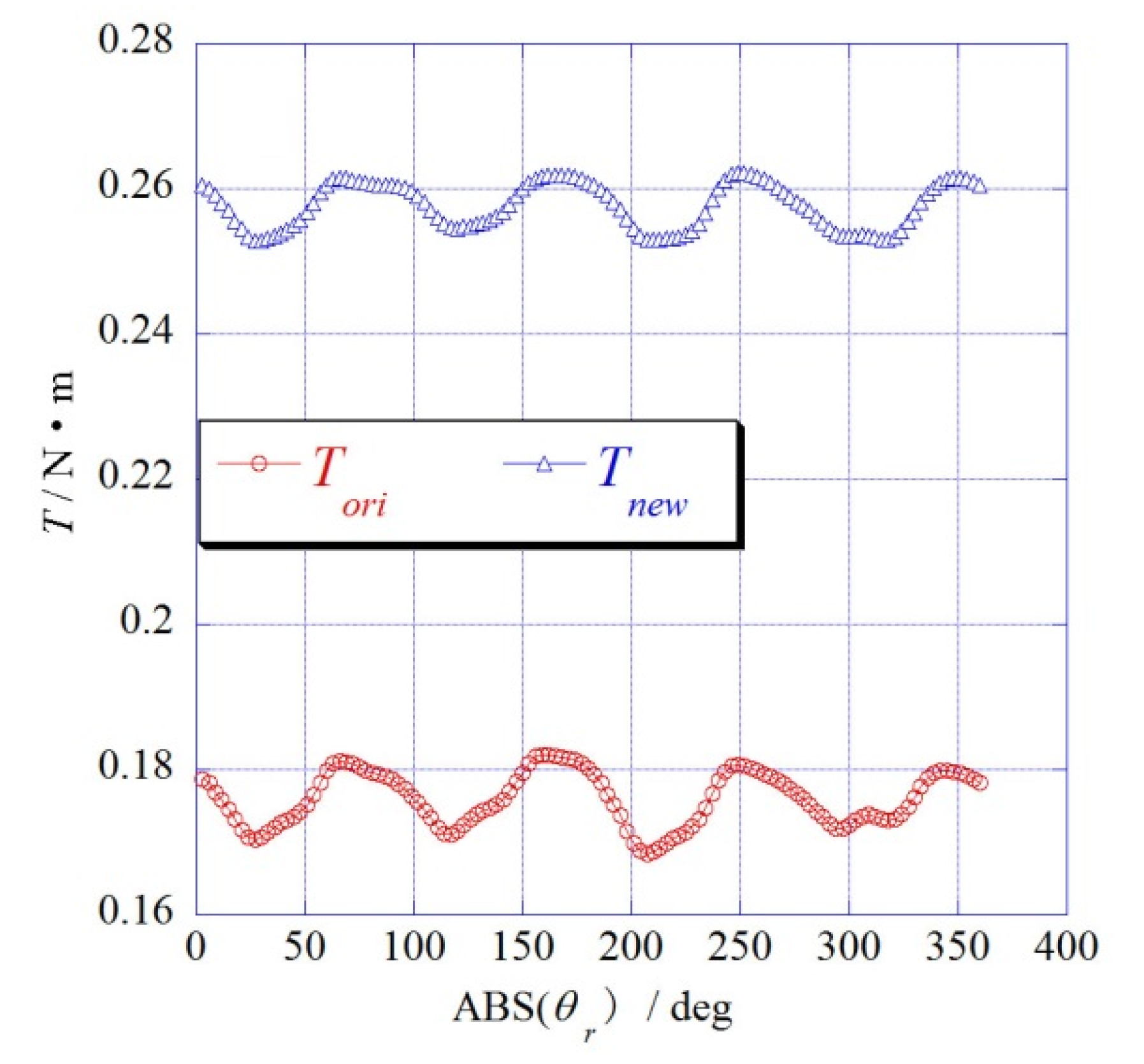
- The flow is more crowded at the tip clearance of the original model by reflections of the pressure distribution at tip clearance area. The turbulent kinetic energy is changed to pressure potential energy and can’t be used to output the torque of the rear rotor. This problem is resolved in the new model, because pressure at the tip clearance area is decreased and the flow is smooth. This can also be demonstrated by the streamlines of original and new models. The high turbulent kinetic energy area of the new model is moved forward, to the middle of the blade. The rear rotor’s torque in the new model is greater than that of original model, and the torque of rear rotor is changed smoothly at the top and bottom of the curve. Therefore, the torque of the rear rotor is enhanced, and rear flow conditions are improved.
Author Contributions
Funding
Acknowledgments
Conflicts of Interest
Nomenclature
| Qd | Design flow rate of the small hydro-turbine |
| Hd | Design head of the small hydro-turbine |
| Pa | Power assumed in a pipe of agricultural water |
| Ha | Head assumed in a pipe of agricultural water |
| Qa | Flow rate assumed in a pipe of agricultural water |
| Q | Flow rate in the experimental apparatus |
| Hdf | Design head of front rotor |
| Hdr | Design head of rear rotor |
| Nf | Rotation speed of front rotor |
| Nr | Rotation speed of rear rotor |
| D | The diameter of the casing |
| Dhf | The hub diameter of front rotor |
| Dtf | The tip diameter of front rotor |
| Dhr | The hub diameter of rear rotor |
| Dtr | The tip diameter of rear rotor |
| Zf | Blade number of front rotor |
| Zr | Blade number of rear rotor |
| B | The blockage ratio of the blade |
| r | Present radius of the front or rear rotor |
| Z | Blade number of the front or rear rotor |
| t | The thickness of front or rear blade |
| θ | The setting angle of front or rear blade |
| ts | The time-step in the numerical analysis |
| rc | The radius of the casing |
| α | The attack angle |
| u | The velocity of the blade |
| βin | The inlet angle |
| Vz | The axial velocity |
| Vt | The circumferential velocity |
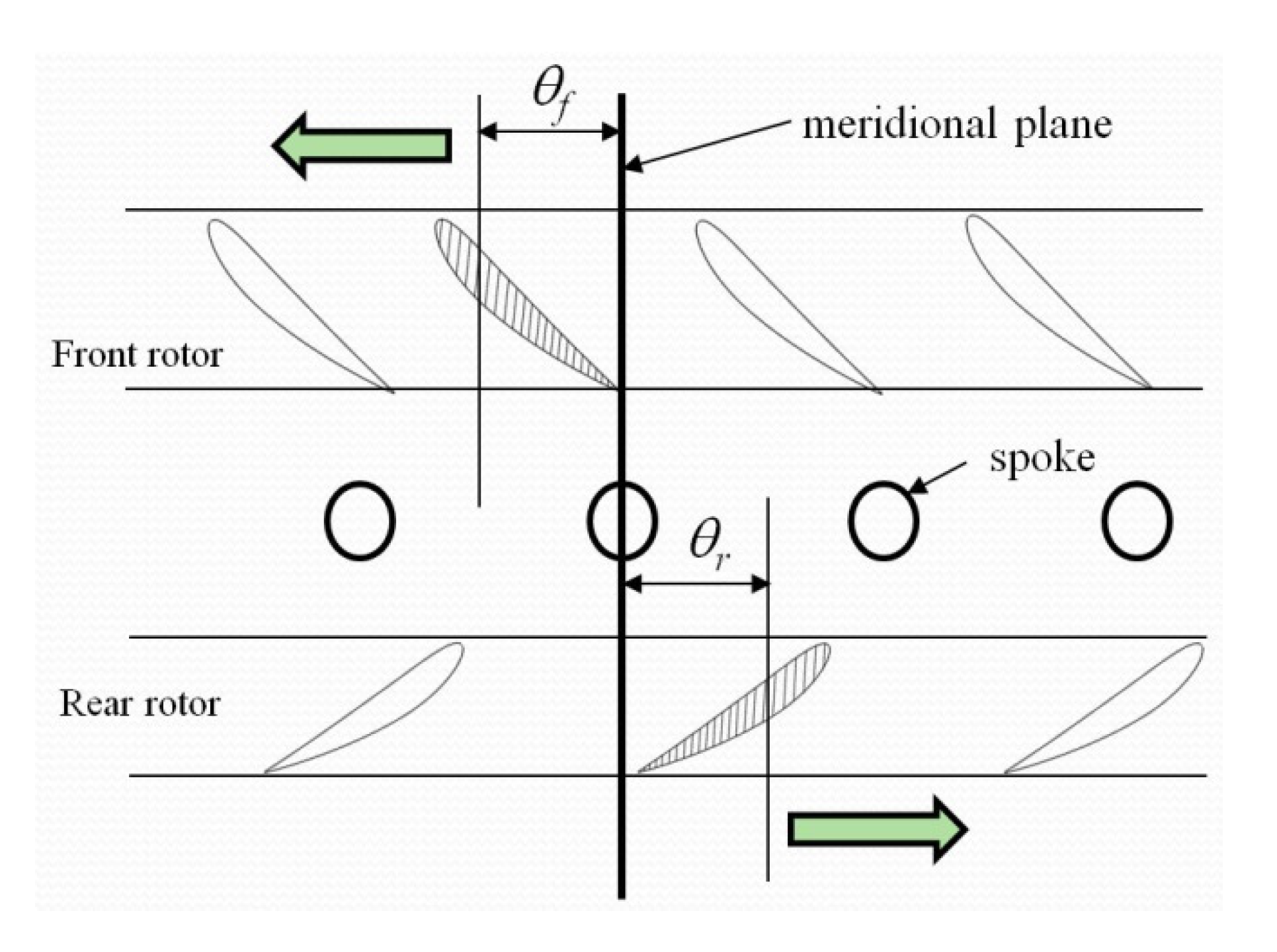
| θf | Base line angle of front rotor |
| θr | Base line angle of rear rotor |
References
- Scott, C.A.; Sugg, Z.P. Global energy development and climate-induced water scarcity—Physical limits, sectoral constraints, and policy imperatives. Energies 2015, 8, 8211–8225. [Google Scholar] [CrossRef]
- Furukawa, A.; Okuma, K.; Tagaki, A. Basic study of low head water power utilization by using darrieus-type turbine. Trans. JSME 1998, 64, 2534–2540. [Google Scholar] [CrossRef]
- Kanemoto, T.; Inagaki, A.; Misumi, H.; Kinoshita, H. Development of Gyro-type hydraulic turbine suitable for shallow stream (1st Report, rotor works and hydroelectric power generation). Trans. JSME 2004, 70, 413–418. [Google Scholar] [CrossRef]
- Kei, T.; Kotaro, H.; Kai, S.; Satoshi, W.; Daisuke, M.; Akinori, F. A study on darrieus-type hydro-turbine toward utilization of extra-low head natural flow streams. Intern. J. Fluid Mach. Syst. 2013, 6, 152–159. [Google Scholar] [CrossRef]
- Daisuke, M.; Kei, T.; Satoshi, W.; Kusuo, O.; Akinori, F. Experimental and numerical investigations on performances of darriues-type hydro-turbine with inlet nozzle. Intern. J. Fluid Mach. Syst. 2014, 7, 151–159. [Google Scholar] [CrossRef]
- Matsui, J. Internal flow and performance of the spiral water turbine. Turbomachinery 2010, 38, 358–364. [Google Scholar]
- Ikeda, T.; Iio, S.; Tatsuno, K. Performance of nano-hydraulic turbine utilizing waterfalls. Renew. Energy 2010, 35, 293–300. [Google Scholar] [CrossRef]
- Nakajima, M.; Iio, S.; Ikeda, T. Performance of savonius rotor for environmentally friendly hydraulic turbine. J. Fluid Sci. Technol. 2008, 3, 420–429. [Google Scholar] [CrossRef]
- Iio, S.; Uchiyama, F.; Sonoda, C.; Ikeda, T. Performance improvement of savonius hydraulic turbine by using a shield plate. Turbomachinery 2009, 37, 743–748. [Google Scholar]
- Iio, S.; Oike, S.; Sato, E.; Ikeda, T. Failure events in the field text of environmentally friendly nano-hydraulic turbines. Turbomachinery 2011, 39, 162–168. [Google Scholar]
- Kanemoto, T.; Kaneko, M.; Tanaka, D.; Yagi, T. Development of counter-rotating type machine for water power generation (1st Report, counter-rotating type generator and axial-flow runners). Trans. JSME 2000, 66, 1140–1146. [Google Scholar] [CrossRef]
- Kanemoto, T.; Tominaga, K.; Tanaka, D.; Sato, T.; Kashiwabara, T.; Uno, M. Development of counter-rotating type machine for hydroelectric power generation (2nd Report, hydraulic performance and potential interference of counter-rotating runners). Trans. JSME 2002, 68, 3416–3423. [Google Scholar] [CrossRef]
- Tanaka, D.; Kanemoto, T. Development of counter-rotating type machine for hydroelectric power generation (3rd Report, design materials for solidity of axial flow runners). Trans. JSME 2006, 72, 686–692. [Google Scholar] [CrossRef]
- Creech, A.C.W.; Borthwick, A.G.L.; Ingram, D. Effects of support structures in an LES actuator line model of a tidal turbine with contra-rotating rotors. Energies 2017, 10, 726. [Google Scholar] [CrossRef]
- Shigemitsu, T.; Fukutomi, J.; Tanaka, C. Renewable Energy in the Service of Mankind; Springer International Publishing: Cham, Switzerland, 2015; Volume I. [Google Scholar]
- Sonohata, R.; Fukutomi, J.; Shigemitsu, T.T. Study on the contra-rotating small-sized axial flow hydro turbine. Open J. Fluid Dyn. 2012, 2, 318–323. [Google Scholar] [CrossRef]
- Shigemitsu, T.; Fukutomi, J.; Sonohata, R. Performance and internal flow of contra-rotating small hydro turbine. In Proceedings of the ASME Fluids Engineering Division Summer Meeting, Incline Village, NV, USA, 7–11 July 2013. [Google Scholar]
- Shigemitsu, T.; Fukutomi, J.; Tanaka, C. Unsteady flow condition of contra-rotating small-sized hydro turbine. In Proceedings of the 12th Asian International Conference on Fluid Machinery, Yogyakarta, Indonesia, 25–27 September 2013. [Google Scholar]
- Shigemitsu, T.; Takeshima, Y.; Tanaka, C.; Fukutomi, J. Influence of spoke geometry on performance and internal flow of contra-rotating small-sized hydroturbine. In Proceedings of the ASME/JSME/KSME Joint Fluids Engineering Conference, Seoul, Korea, 26–31 July 2015. [Google Scholar]
- Nan, D.; Shigemitsu, T.; Zhao, S.D.; Takeshima, Y. Numerical analysis of contra-rotating small hydro-turbine with cylinder spoke. Int. J. Fluid Mach. Syst. 2018, 11, 21–29. [Google Scholar] [CrossRef]
- Nan, D.; Shigemitsu, T.; Zhao, S.D.; Takeshima, Y. Internal flow and performance with foreign vegetable materials in a contra-rotating small hydro-turbine. Int. J. Fluid Mach. Syst. 2017, 10, 385–393. [Google Scholar] [CrossRef]
- Nan, D.; Shigemitsu, T.; Zhao, S.D.; Ikebuchi, T.; Takeshima, Y. Study on performance of contra-rotating small hydro-turbine with thinner blade and longer front hub. Renew. Energy 2018, 117, 184–192. [Google Scholar] [CrossRef]
- Gabl, R.; Innerhofer, D.; Achleitner, S.; Righetti, M.; Aufleger, M. Evaluation criteria for velocity distributions in front of bulb hydro turbines. Renew. Energy 2018, 121, 745–756. [Google Scholar] [CrossRef]


| Rotor | Parameter | Hub | Mid | Tip |
|---|---|---|---|---|
| Front Rotor | Diameter (mm) | 29 | 43.5 | 58 |
| Blade Number | 4 | |||
| Blade Profile | NACA65 | |||
| Solidity | 1.4 | 1.07 | 0.85 | |
| Setting Angle (°) | 25.5 | 20 | 15.8 | |
| Rear Rotor | Diameter (mm) | 29 | 43.5 | 58 |
| Blade Number | 3 | |||
| Blade Profile | NACA65 | |||
| Solidity | 0.86 | 0.71 | 0.59 | |
| Setting Angle (°) | 44.6 | 29.7 | 18.9 | |
| R (mm) | Blade Thickness Over Blade Length of Original Model (%) | Blade Thickness Over Blade Length of New Model (%) | Original Blockage Ratio of Front Blade (%) | New Blockage Ratio of Front Blade (%) | Original Blockage Ratio of Rear Blade (%) | New Blockage Ratio of Rear Blade (%) |
|---|---|---|---|---|---|---|
| 29 | 12 | 12 | 90.52 | 90.52 | 92.89 | 92.89 |
| 26.1 | 12 | 11.44 | 90.05 | 90.52 | 92.54 | 92.89 |
| 23.2 | 12 | 10.8 | 89.46 | 90.52 | 92.10 | 92.89 |
| 20.3 | 12 | 10.08 | 88.71 | 90.52 | 91.53 | 92.89 |
| 17.4 | 12 | 9.26 | 87.71 | 90.52 | 90.78 | 92.89 |
| 14.5 | 12 | 8.31 | 86.30 | 90.52 | 89.73 | 92.89 |
© 2018 by the authors. Licensee MDPI, Basel, Switzerland. This article is an open access article distributed under the terms and conditions of the Creative Commons Attribution (CC BY) license (http://creativecommons.org/licenses/by/4.0/).
Share and Cite
Nan, D.; Shigemitsu, T.; Zhao, S. Investigation and Analysis of Attack Angle and Rear Flow Condition of Contra-Rotating Small Hydro-Turbine. Energies 2018, 11, 1806. https://doi.org/10.3390/en11071806
Nan D, Shigemitsu T, Zhao S. Investigation and Analysis of Attack Angle and Rear Flow Condition of Contra-Rotating Small Hydro-Turbine. Energies. 2018; 11(7):1806. https://doi.org/10.3390/en11071806
Chicago/Turabian StyleNan, Ding, Toru Shigemitsu, and Shengdun Zhao. 2018. "Investigation and Analysis of Attack Angle and Rear Flow Condition of Contra-Rotating Small Hydro-Turbine" Energies 11, no. 7: 1806. https://doi.org/10.3390/en11071806
APA StyleNan, D., Shigemitsu, T., & Zhao, S. (2018). Investigation and Analysis of Attack Angle and Rear Flow Condition of Contra-Rotating Small Hydro-Turbine. Energies, 11(7), 1806. https://doi.org/10.3390/en11071806