1. Introduction
In the field of electrical drive high-power applications, a very common control method for AC drives is direct torque control (DTC) [
1,
2]. Because it suffers from a few disadvantages like high flux and torque ripple or varying switching frequency, plenty of developed modifications striving to eliminate these disadvantages are known [
3]. Because the switching losses are significant in high-power drives, the low switching frequency of the transistors must be used. In some applications, this average switching frequency can go as low as 500 Hz for IGBT inverter [
4]. In this low switching frequency operation, it is necessary to ensure that all applied switching combinations have effect in the desired way.
Sometimes, the DTC algorithm might be unable to choose the correct vector that would push the system toward given references. So, the DTC method causes unnecessary flux and torque ripples. The flux plane is divided into six sectors, and the rotating flux vector sequentially passes through all of them. Some problems occur at the borders between two flux sectors. Approaches for how to choose the correct vector in these states were invented. The most successful of them were dividing the plane of flux vector into more sectors than the conventional six [
5], modifying the switching table or the commands for the table [
6,
7], using voltage vector selection according to fuzzy logic [
8], reducing the number of voltage vector changes [
9], changing the torque and flux band online according to the actual state of the motor [
10], overriding the voltage sag [
11], and applying the sector shift or rotation by certain angle [
12]. Another problematic feature occurs within the flux sector. The DTC method a priori neglects some voltage vectors. It always chooses from only six vectors, even though there are eight possibilities. In order to eliminate the problem, the strategy can be adjusted to use the space vector modulation (SVM-DTC) [
3] that does not have this limitation, or an extended switching table with multiple sectors can be utilized [
13]. This paper deals with the conventional type of this method [
1]. The two-state hysteresis controller of flux amplitude and the three-state hysteresis controller of torque are utilized to choose the appropriate voltage vector from the look-up table.
Model Predictive Control (MPC) is not a new concept. It has been used in other industries, mostly in chemical applications to control the transients of dynamic systems [
14,
15]. In these applications, there is a lot of time for calculations, because of its long time constants, so this kind of control was possible. When the computational power of microcontrollers became sufficient, this concept was introduced to power converters [
16]. Soon after that, the usage of MPC was extended to electric motors [
17,
18,
19,
2021]. Today, it is a very promising strategy for motor control, as it enables to optimize multiple parameters and offers operation with non-linear systems [
22]. Moreover, the upgrade from the existing system is easy as it does not require any hardware modification, and only a software change is necessary. MPC in electric drives can be used in wide spectrum of applications. The prospective ones are in a sensorless operations of the drive [
23], optimization of switching frequency [
24], prediction for longer predicted horizon [
25,
26], and the operation of multilevel inverters [
27]. MPC is also usable in low switching frequency operation [
24,
28,
29,
30].
The MPC algorithm for the induction motor drive control is distinguished as two realizations: predictive torque control (PTC) and predictive current control (PCC). The PTC method controls the torque and flux, which is similar to DTC, and the PCC method controls two components of the current, which is similar to Field Oriented Control (FOC). The behaviors of these strategies were compared to each other [
31,
32,
33], and the better performance of MPC was observed. When talking about MPC in connection with electrical drives, the PTC realization is usually meant. This paper deals with the often-implemented type of PTC method that utilizes an observer, a control variable prediction, and a cost function [
17]. No voltage vector modulation is utilized, and the selected vector is applied for the whole sample time. Therefore, we will continue using the abbreviation PTC.
PTC seems to achieve better results, and the waveforms of control variables (torque and flux amplitude) are smoother than in DTC [
22,
31,
32,
33,
34,
35]. Compared to the other works, the paper analyzes the switching pattern in greater detail in order to identify the influence on the waveforms. It looks at which vector is applied in what kind of situations. It finds two major situations where the strategies react differently. The first one deals with the voltage vector selection in the same flux sector, and the second one analyses the vector selection when crossing the border between two flux sectors. The effect of the applied voltage vector on the drive performance is investigated. This paper shows that, in the DTC case, the voltage vector that would not bring the desired effect can be applied. It also shows that, in the PTC case, the effect of each vector is predicted in advance, and the better voltage vector is applied, so the ripple in the waveforms is smaller. This paper focuses on small switching frequencies, so each applied voltage vector is important, and each switching is noticeable. The results were verified by simulation comparison of the trajectories of the flux vectors. Then, the experiment with PTC was run in order to show whether PTC selects better voltage vectors and whether the torque waveform is smoother.
2. Control Methods
The examined predictive method (PTC) [
17] controls the torque developed by the induction motor and its stator flux vector amplitude. The same variables are controlled by the examined conventional DTC [
1] as well as by most DTC modifications mentioned in the introduction. Because of that, a lot of characteristics of these two control strategies are similar. PTC evaluates the effects of all input voltage vectors and chooses the best one according to the defined criteria—in the given case, the difference between references and real values of torque and flux amplitude. The induction motor inputs are voltage vectors, and the used power voltage source inverter is able to deliver eight voltage vectors. Six of them are active vectors with non-zero voltage value, and two of them are passive vectors with zero voltage value.
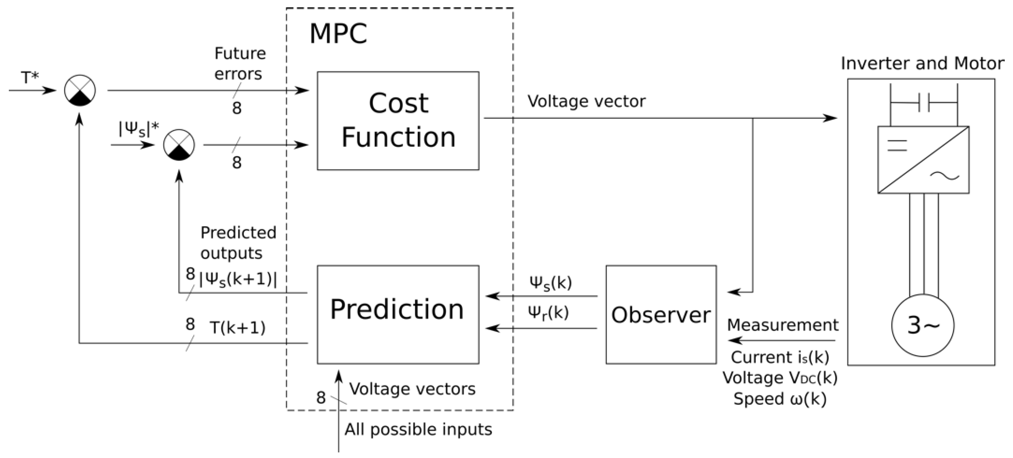
The control algorithm consists of several blocks. They are the observer of the induction motor actual state, the predictive model that calculates the induction motor response to any possible input, and the rules for the final voltage vector selection (cost function). The block diagram is presented in
Figure 1.
The first step is to obtain the actual state of the motor. The required values are vectors of the rotor and stator fluxes and torque. It is not practical to measure them directly; they must be estimated. The only measured values are the stator currents, voltage level in DC link, and mechanical speed of the rotor. The induction motor is described by a set of known equations [
36] from which the observer can be designed [
37]. The commonly used one is the Luenberger observer [
38].
Then, the prediction takes part. There are eight possibilities of voltage vectors
vs(
n) where n is a number from 0 to 7 and represents the predicted voltage vector. For all of them, the current vector
is(
k + 1) must be predicted. The possible future stator current is calculated from the measured current, values of estimated rotor flux
ψr(
k) and electrical motor speed
ω(
k) according to Equation (1) as:
where
Ts is the sample time, τ
σ is the time constant calculated as
τσ = σ·
Ls/
Rσ, σ is a leakage factor,
Rσ is a resistance
Rσ =
Rs +
Rr·
kr2,
Ls is stator inductance,
Rs is a stator winding resistance,
Rr is a rotor winding resistance,
kr is the inductance coefficient
kr =
Lm/
Lr,
Lm is mutual inductance of stator and rotor,
Lr is a rotor inductance, and
τr is rotor time constant
τr =
Lr/
Rr.
The controlled variables in PTC are the same as in DTC. The torque
T and the stator flux amplitude |
ψs| are supposed to be maintained at their references. Therefore, the value of torque and stator flux must be predicted as well. They are predicted according to Equations (2) and (3) as
and
where
pp is the number of pole pairs of the motor. Equations (2) and (3) give the prediction of control variables, which says what flux and torque we get when deciding for a certain voltage vector.
Then it is necessary to choose the one that would be applied on inverter. In order to find the best one, all of the states will receive points by cost function. These points say how far the predicted state is from the ideal demanded state defined by the references of the flux amplitude and torque. The bigger the value, the further the state is from the references. So, the lower value is the better one. The cost function g is expressed in Equation (4) as
The coefficient
k in Equation (4) determines what impact the two parts of the equation have on the resulting value. It is usually chosen as a fraction of nominal torque and nominal flux amplitude of the motor Equation (5):
It ensures that both parts have the same impact on the result. Finally, the voltage vector with minimum value of the cost function is selected to be applied in the next step.
3. Comparison of Switching Patterns
In case of the examined DTC method [
1], the selection of the voltage vector is done according to the very simple switching table. The actual voltage vector is selected by means of the torque and flux hysteresis controllers and flux sector. The switching table is given by
Table 1 and the situation is depicted in
Figure 2. In this case, the drive performance is sufficient for most time of the induction motor running time and the selected voltage vector is identical for both PTC and DTC methods.
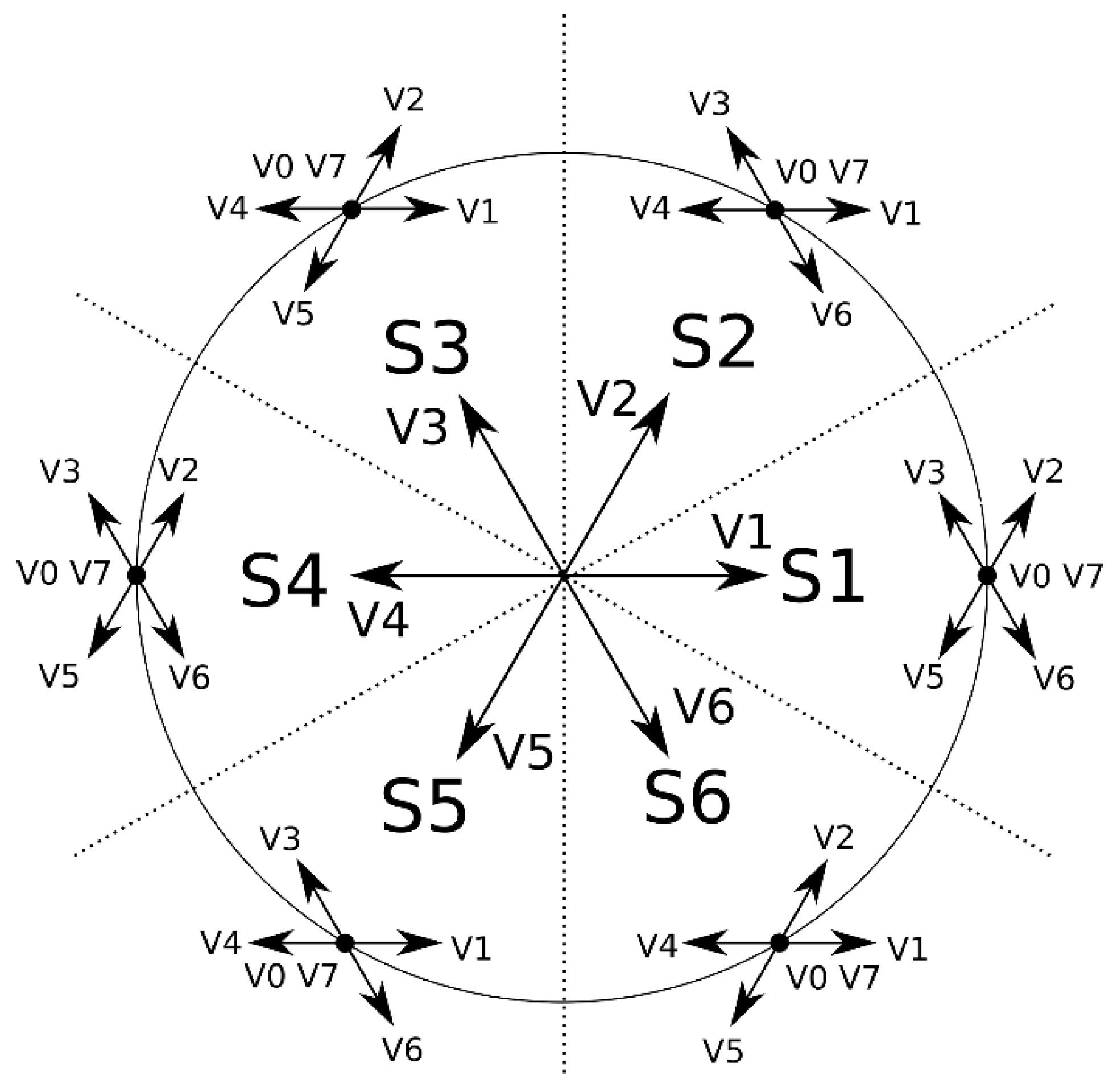
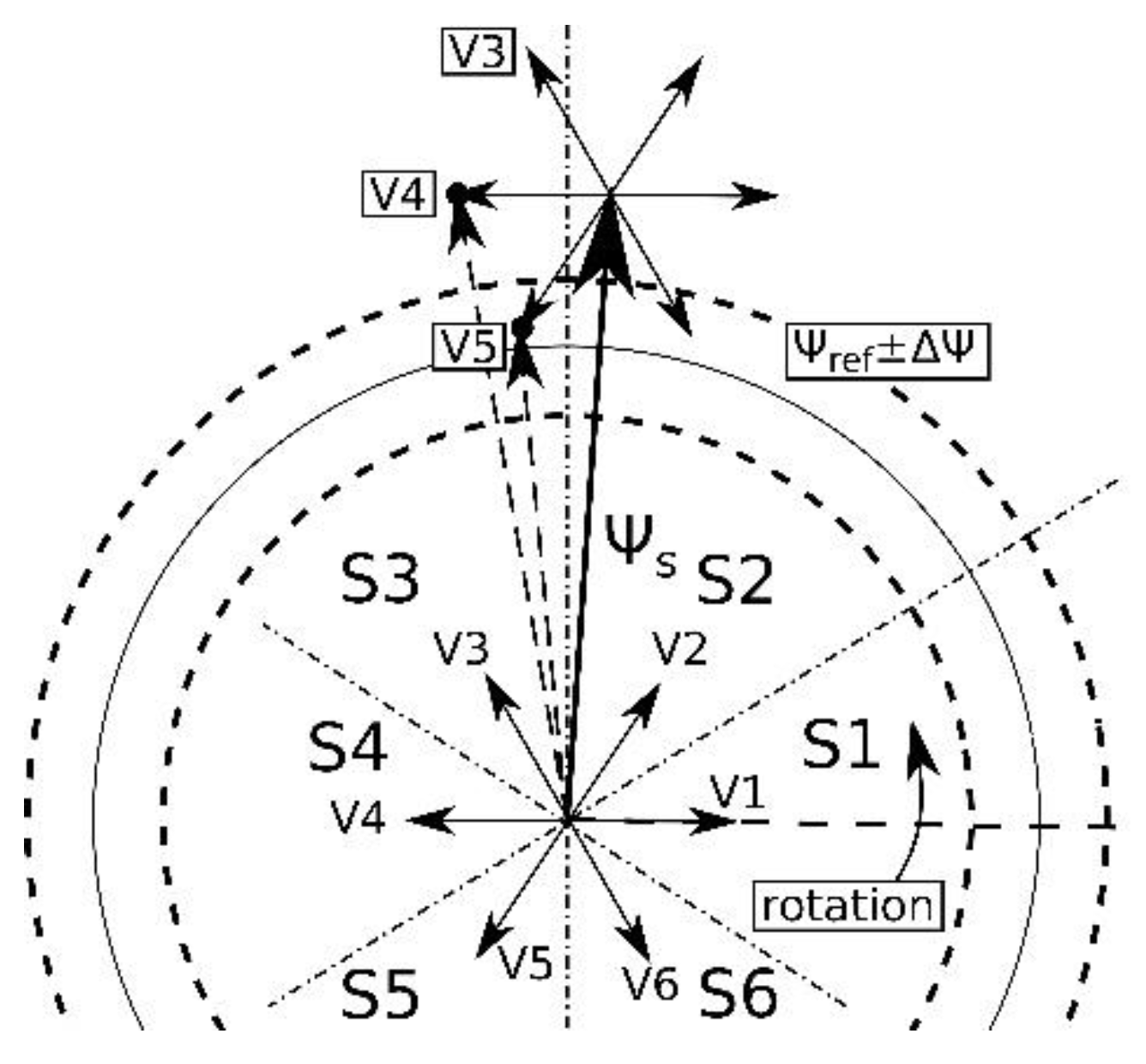
In the following part, the process of voltage vector selection for one sector is described in detail. The tip of the stator flux vector is regarded to be placed to the sector S2. In case of the DTC algorithm, one of the six vectors (four active and two passive) is chosen. The effect of these six vectors is determined. Vectors V1, V3, V4, and V6 are selected when the flux level and torque changes are demanded. When the torque value lies within the hysteresis limits, the algorithm chooses passive vector V0 or V7. The algorithm uses neither vectors V2 nor vector V5 in this case. The situation is illustrated in
Figure 2. The applied and unapplied voltage vectors for each flux sector are summarized in
Table 2.
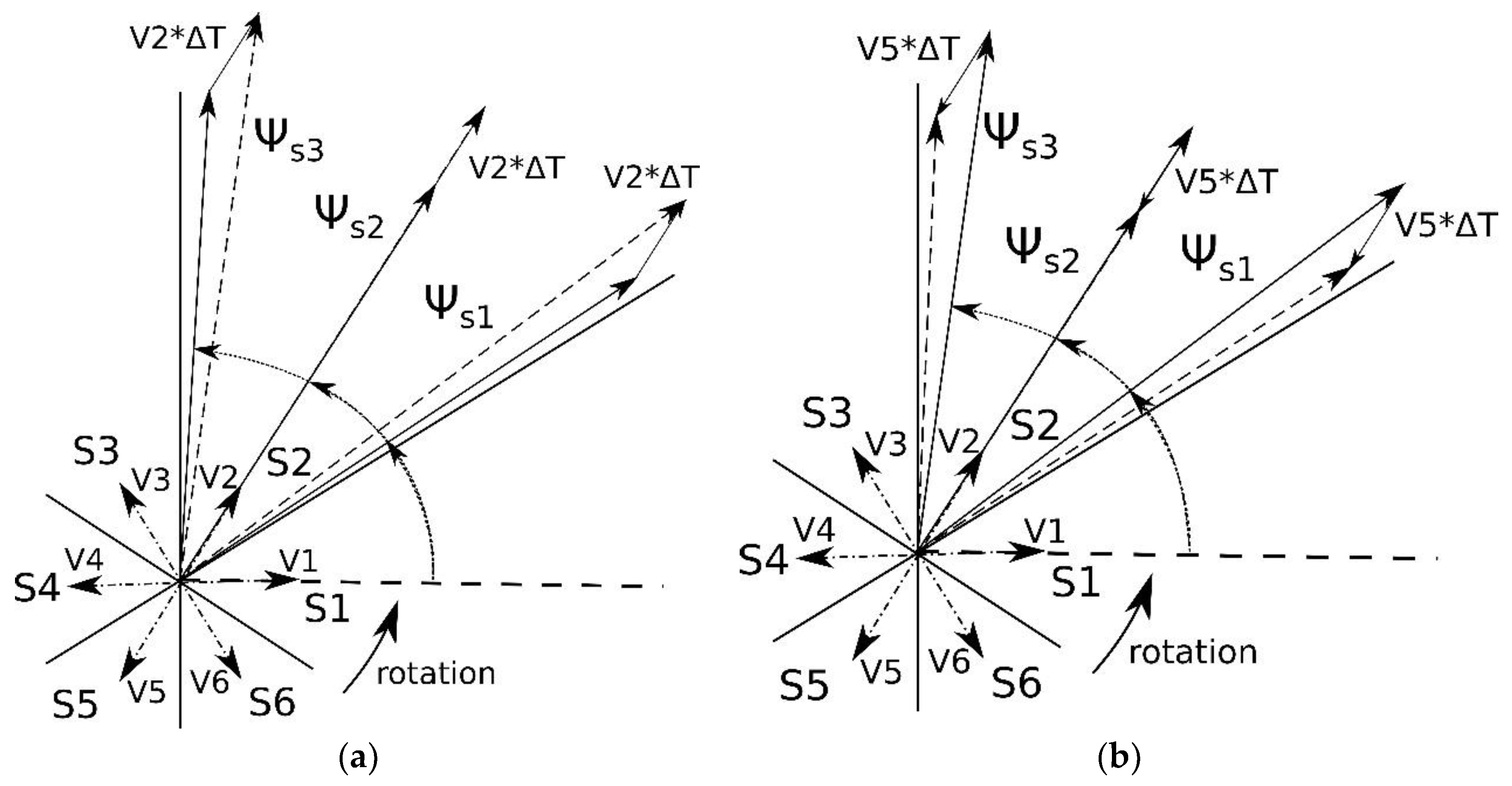
The effect of the unapplied vectors V2 and V5 is not that simple and depends on the exact position of the flux vector in the sector. In case of DTC, the actual position of the vector in the sector is not known. The vector effect is different at the beginning, in the middle or at the end of the sector. The effect of the vector V2 in the sector S2 is illustrated in
Figure 3a. The vector
Ψs1 is located at the beginning of the sector S2. Applying the voltage vector V2 will increase the flux amplitude and slightly increase the torque. The flux vector
Ψs2 is located in the middle of the sector S2, and the only effect will be the flux level increase. The flux will be increased more than in other two cases. The last vector
Ψs3 is located near the end of the sector. The effect of V2 will result in flux level increase and the torque will be slightly reduced. The voltage vector V2 exact effect is not determined in case of DTC, and therefore the vector V2 in the sector S2 is unapplied.
The effect of the opposite vector V5 in the flux sector S2 (shown in
Figure 3b) is very similar. It also depends on the flux vector exact position. In all positions of the sector, the flux level will be reduced, and the torque will be modified in the same way as in the previous case. Therefore, the vector V5 in the sector S2 is unapplied as well.
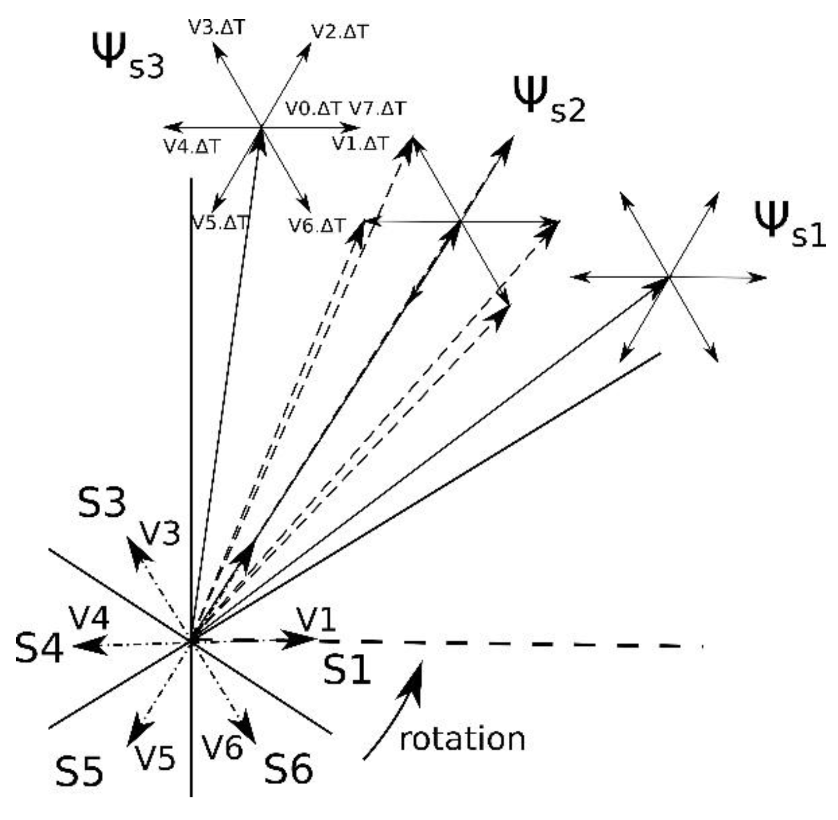
In case of the examined predictive method (PTC) [
17], the full effect of each vector is predicted at first. Then, these effects are evaluated according to the given cost function (4) and the most suitable one is selected. There is not a reason to ignore the two voltage vectors in any sector, so all eight voltage vectors can be applied. The situation is depicted in
Figure 4.
As a result, in the case of PTC, all eight possible voltage vectors (six active and two passive) can be applied in any instant. In the case of DTC, only six voltage vectors (four actives and two passive) can be applied in any flux sector.
The other situation worth analyzing is shown in
Figure 5. The flux vector is approaching toward the end of the sector. Assume that the flux is at the end of the sector S2 and the hysteresis controllers demand the torque increase and the flux level decrease. Then, the voltage vector V4 (according to
Table 1) is applied. This particular voltage vector V4 remains applied for the whole time between control steps. For the whole duration between the control steps, this particular vector, V4, is on the inverter. The flux vector starts to move in the direction of the vector V4, which causes a torque increase and a flux level decrease. The flux vector comes toward the end of the sector and then crosses it. After sector crossing, the new sector S3 is entered, and the voltage vector V4 remains applied. According to
Table 1, it correctly leads to the torque increase but also to the flux level increase. However, it is not the effect demanded by the hysteresis controllers. The PTC method will predict the position of all eight possible flux vectors. According to the given cost function (4), the voltage vector V5 will be selected as the most suitable one. On contrary, in case of DTC method, the voltage vector V4 that is not convenient for the given requirements will be selected.
There are six sectors, and this problem can happen in every transition between them. So, it can appear six times per one flux rotation. The negative effect of this problem also increases with longer sample time because the flux vector moves by bigger steps and the resulting waveforms ripple increase.
4. Results and Discussion
The performance of the drive for both control strategies were simulated in the Matlab Simulink environment. The simulations were carried on a four-pole 5.5 kW induction motor. The nominal values of the motor and the parameters of its equivalent circuit are presented in
Table 3. The reference torque was 30 Nm, flux amplitude 1 Wb and the drive was kept at 140 rad/s by applied load. The time-continuous part of the drive (inverter and motor) was simulated with time loop 10 µs. The algorithms had their own timings that were adjusted to maintain similar average switching frequency of the transistors. This frequency was set to be around 550 Hz in order to correspond to the real values used in high-power applications. The algorithm to adjust the average switching frequency was different for both strategies. At DTC, it was adjusted by the hysteresis of flux and torque, and the algorithm was simulated with the control loop 50 µs. At PTC, the average switching frequency was adjusted by the duration of the control loop. As the average switching frequency of both algorithms is speed dependent, it was necessary to set it up for every working point separately.
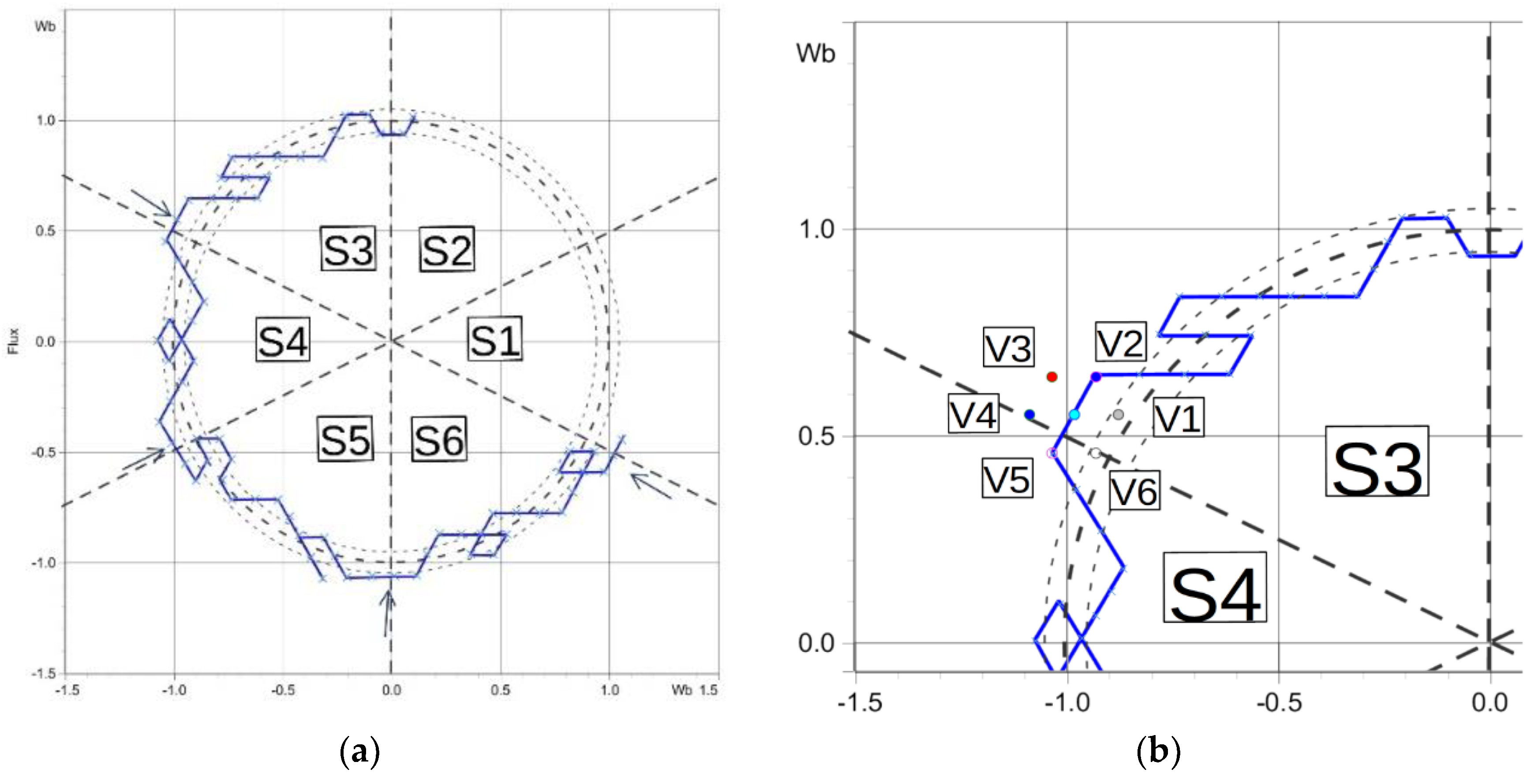
The simulation of the induction motor driven by DTC is presented in
Figure 6. The figure shows the trajectory of stator flux vector tip as the blue curve. Further, it shows the voltage vector selection during flux sector crossing from the old flux sector S3 to the new sector S4. Before the transition, the position of the flux vector is located to the last point in the sector S3. DTC method demands to increase the torque and decrease the flux level. In accordance with
Table 1, the voltage vector V5 is applied. However, as shown in the figure, after applying the voltage vector V5, the flux vector increases its amplitude. The voltage vector that would meet the DTC’s requirements would be vector V6. This situation can happen six times per one flux turn. These points are in the figure marked by arrows.
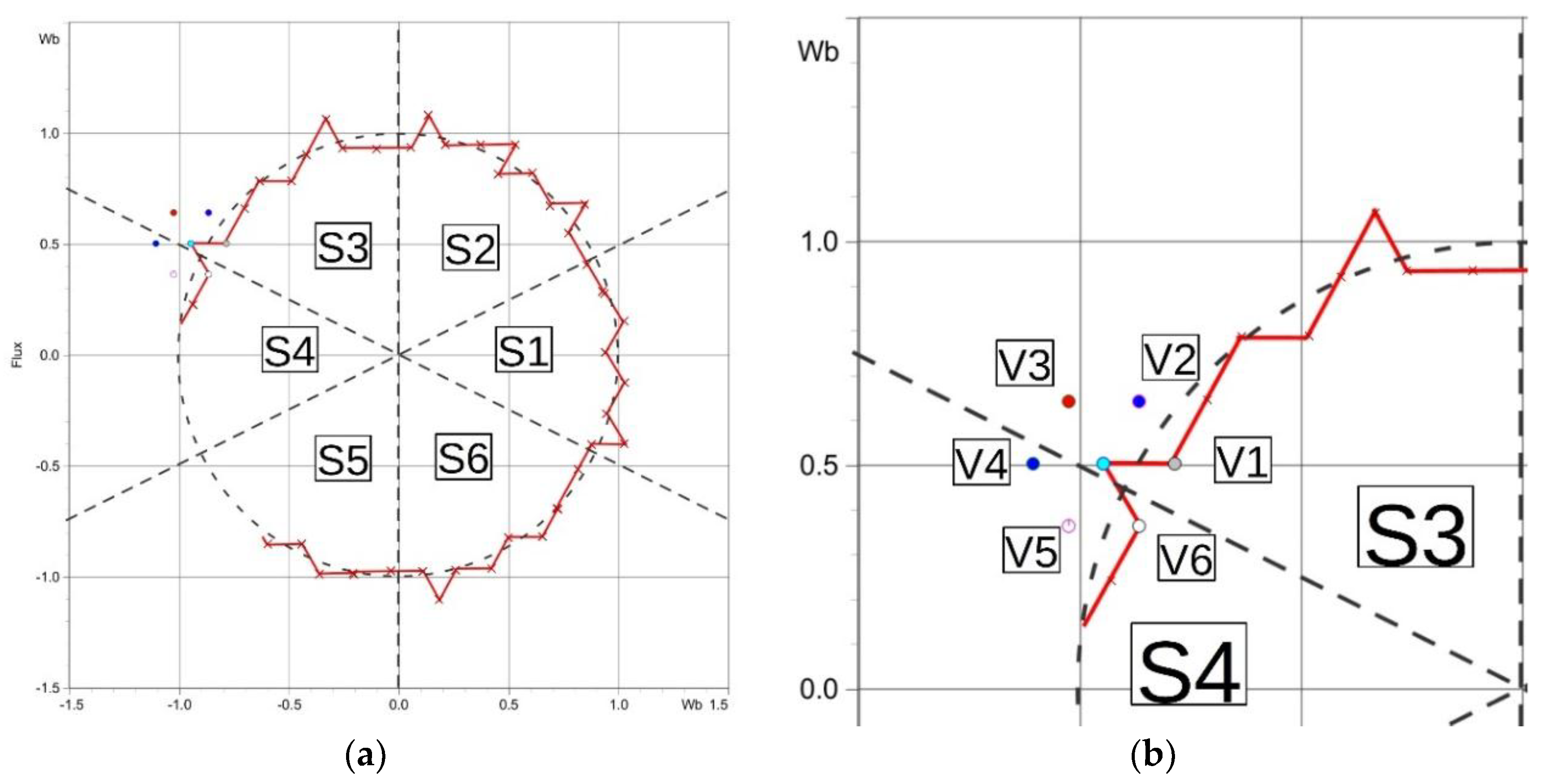
The simulation results of the induction motor driven by DTC are presented in
Figure 7. The figure shows the trajectory of stator flux vector tip and the predicted effect on voltage vectors and flux sectors. The red curve represents the flux sector transition at PTC. At the end of the sector S3, the torque is smaller than the reference torque, and flux level is higher than its reference. Therefore, the results of the hysteresis controllers (DTC) and cost function (PTC) would be the torque increase and flux decrease. According to
Table 1, in sector S3, the voltage vector V5 would be applied in case of DTC. The flux vector tip would move in the direction of V5, enter the new sector S4, and continue in the same direction. The effect of the applied vector V5 in the new sector S4 differ from effects in the old sector S3. The new effect is the torque and flux increases. Finally, the results are the increased torque and increased flux (the same as in
Figure 5). In case of PTC, the trajectory of the flux vector tip is predicted for all vectors and the applied voltage vector is selected according to the predicted flux vector tips. This is calculated by the cost function (4). The result of the cost function calculation represents the difference between the predicted torque and flux values and their references. So, the lower value the more convenient voltage vector. In this case, the most suitable vector V6 was selected, as it receives the least value. The results of the cost function calculation are presented in
Table 4.
As shown in
Table 2 and in
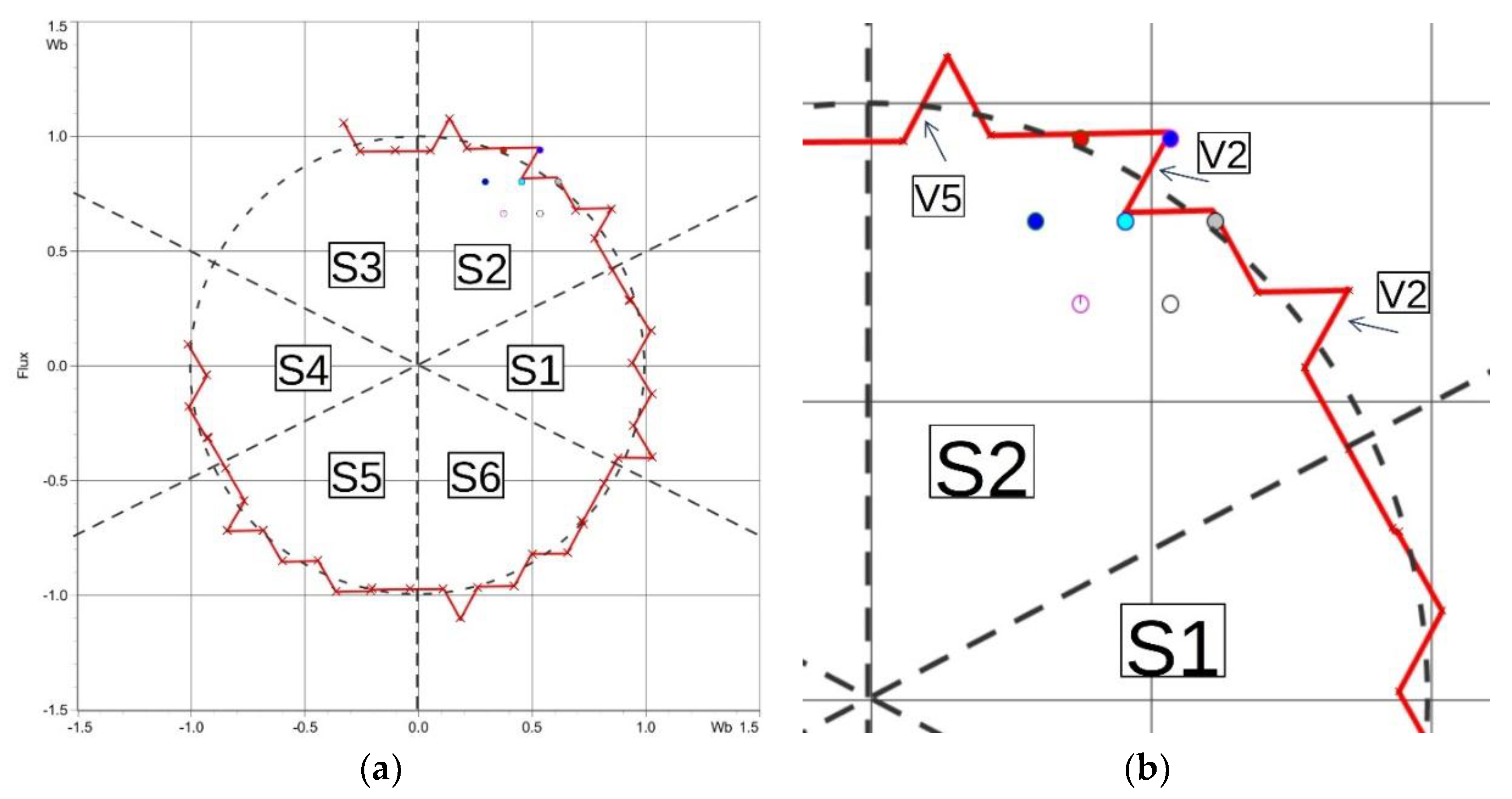
Figure 2, in case of DTC, six voltage vectors can be applied, and two of them may not be applied. But under certain conditions, one of these two unapplied vectors can bring the controlled variables closer to the references than the rest of the vectors. In
Figure 8, a part of the trajectory of the flux vector tip is shown. At the marked point, the position of flux vector is predicted for the next step for all eight voltage vectors. The flux vector is located in sector S2, and the DTC controllers demand to increase the flux amplitude and increase the torque. According to
Table 1, the voltage vector V3 is selected in DTC case. In the PTC case, vector V2 was applied.
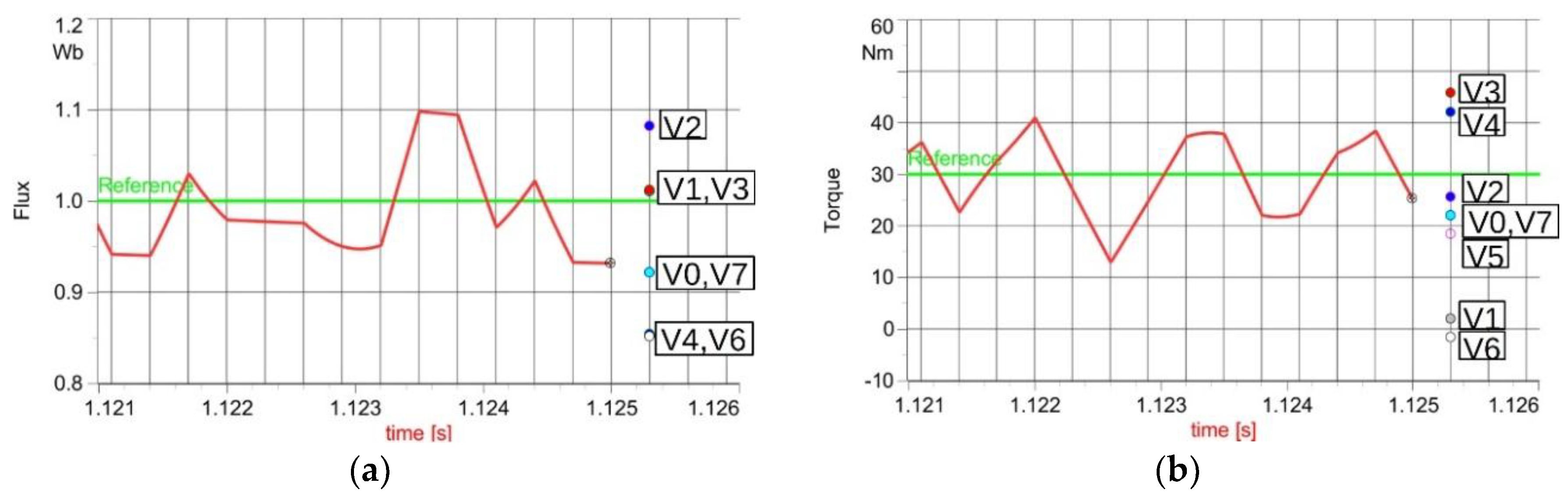
The explanation of the vector selection in the PTC case is shown in
Figure 9. It shows the waveform of stator flux amplitude and developed torque at the PTC run. Further it shows all possible predicted values of torque and flux level for the next step. In case of DTC, the vector V3 would be applied to increase both the torque and the flux level. As a result, the flux would be slightly higher than the reference and torque will be much higher than the reference (shown as the red dot in the figure). The vector V2, selected in case of PTC, increases the flux and almost does not change the torque. It results in much higher flux and slightly smaller torque compared to their references (shown as the blue dot in the figure). The cost function (4) was calculated for all vectors. The result value shows that the voltage vector V2 brings the motor closer to the ideal state described by the references as it receives the lowest value. All results of the cost function for this case are presented in
Table 5.
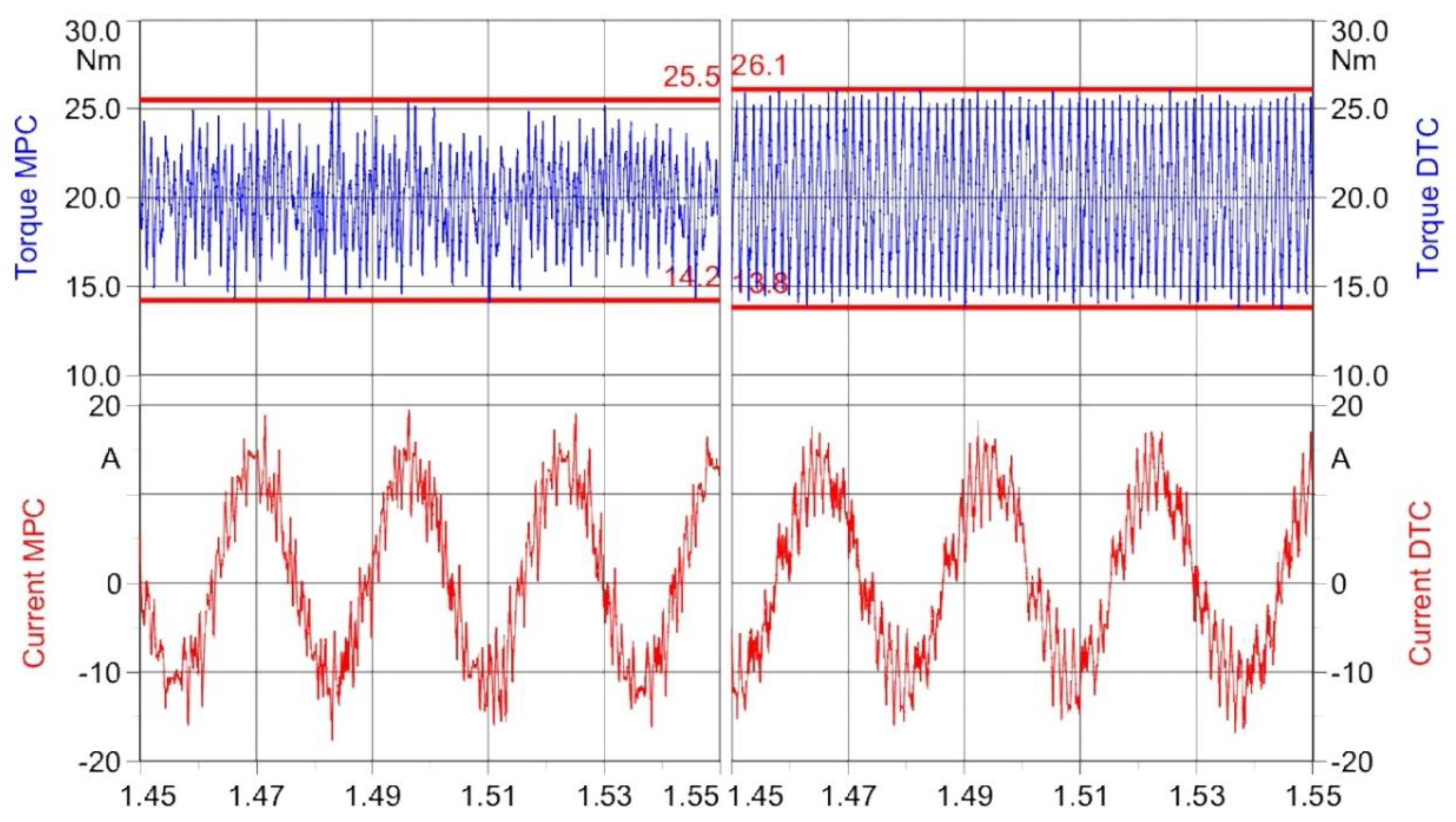
Finally, the experiment was done in order to further verify the simulations. It was carried out on a motor with the same parameters as in the simulation. The inverter of the voltage 540 V in the DC link was controlled by the dSPACE ds1103 system (ds1103, dSpace Inc., Wixom, MI, USA). The same conditions were applied for both algorithms. The drive was kept at 1000 rpm with the applied load 20 Nm. The same average switching frequency was maintained. It was set by the hysteresis width, in the DTC case, and by the duration of the control loop, which was 300 µs, in the PTC case. With the used hardware, the calculation of both strategies takes different time periods. With DTC, the calculation takes 11 µs, and 28 µs with PTC. The waveforms of the torque and current were recorded, and they are presented in
Figure 10. The torque ripple with PTC (11.3 Nm) is lower than the ripple with DTC (12.3 Nm) by 1 Nm. The difference measured on the specific laboratory drive was not very high, but the upgrade from existing DTC system is easy because no hardware modification is required, and only a software change is sufficient. When the microprocessor has adequate capability, there is no reason not to upgrade the control system.
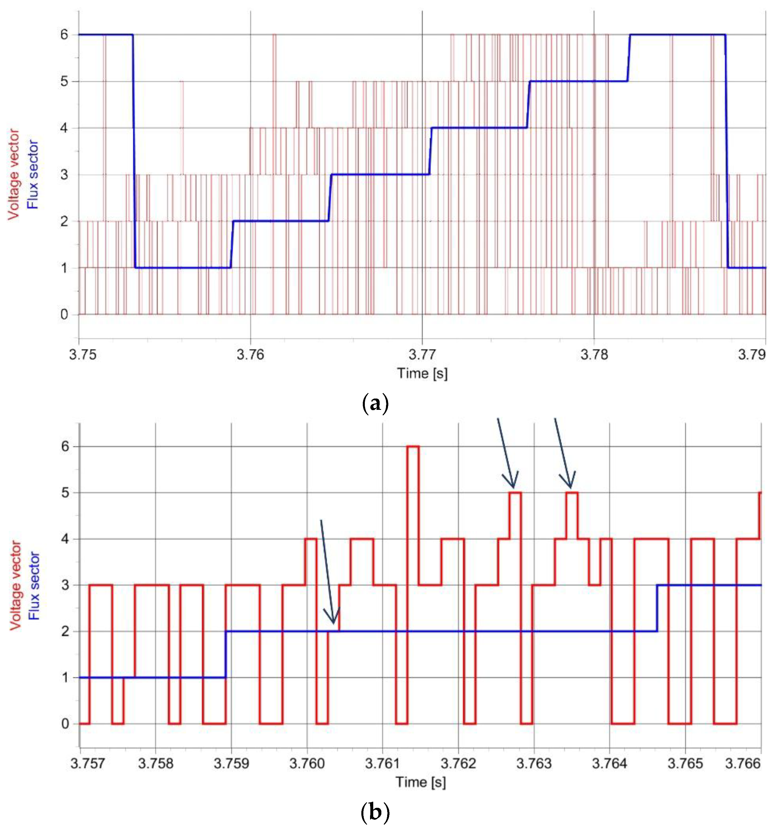
In another experiment, the waveforms of flux sectors and selected voltage vectors over time were observed and are shown in
Figure 11. It shows that the vectors that are never applied at DTC are applied at PTC. The figure shows that the flux vector is located in sector S2, and within this sector, the examined vector V5 is chosen two times and V2 once. They are marked by arrows.
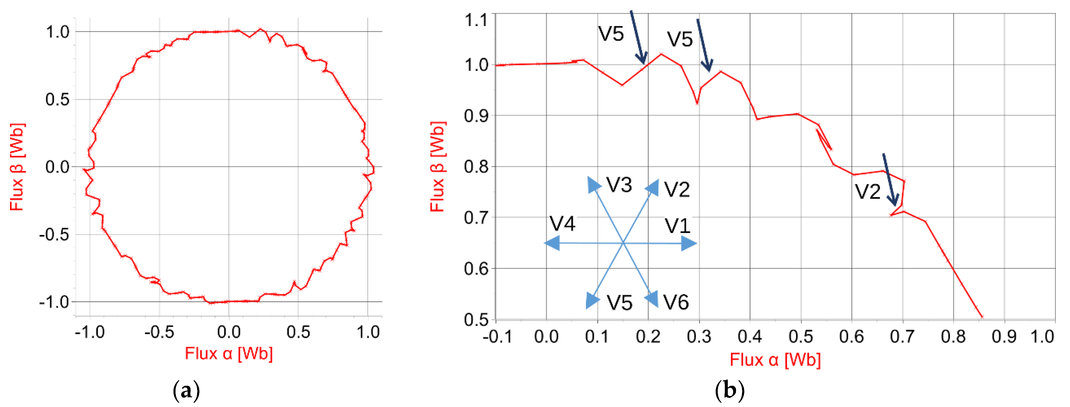
The flux vector tip trajectory at the MPC and the detail of the trajectory curve in the sector S2 corresponding to
Figure 11 is shown in
Figure 12. The vector tip path is defined by the chosen vectors. The path does not always point directly in the chosen vector direction because of the influence of the voltage drop on stator winding. The vectors unapplied by DTC are applied at PTC and are marked by arrows in the figure.
5. Conclusions
In this paper, the patterns of the voltage vector selection in the case of direct torque control and model predictive control have been analyzed and compared. The ways of the vector selection in various situations have been presented, analyzed, and compared, as well as the accuracy of compliance with the reference values of torque and flux amplitude. Two main differences in voltage source inverter voltage vector selection have been shown in the comparison of both strategies.
The stator flux plane is divided into six sectors. The first difference occurs during transitions between these flux sectors. It is shown that DTC behavior is problematic and can result in the improper voltage vector selection. This behavior does not push the system toward their references but does exactly the contrary. Further, it is shown that PTC does not have a problem with the flux sector crossing because the voltage vector is selected according to the predicted effects of the vectors. The second difference occurs within the flux sector. In the DTC case, the effects of six voltage vectors in every flux sector are determined and can be applied. The effect of the resulting two vectors is not determined, so they are not present in the switching table and therefore cannot be applied. Only six vectors can be applied at DTC. In the PTC case, the effects of all voltage vectors are calculated, so all eight vectors can be applied. PTC has a wider range of voltage vector options.
The behavior of both methods was simulated in the Matlab Simulink environment. The trajectory of flux vector tip shows both analyzed situations when the methods select voltage vectors differently. It verified that, with DTC, the voltage vector selection during flux sector transition leads the flux away from the reference, and that with PTC, the flux vector always aims toward its reference. Further, it showed that the selection of these voltage vectors that cannot be applied at DTC can be useful to achieve smoother waveforms of torque and that these vectors are applied by PTC.
The experiment was done in order to further verify the theoretical analysis and the simulations. The test was run for both control methods with the same condition and an average switching frequency around 550 Hz. The torque developed by the motor and the phase current were recorded. The smaller ripple was observed in a torque waveform using PTC. Further, the sequences of flux sectors and selected voltage vectors over time were observed. It proves that the voltage vectors unapplied with DTC are applied with PTC.


