Design and Simulation of a Powertrain System for a Fuel Cell Extended Range Electric Golf Car

Abstract

This article analyses the energy behaviour of an electric golf car as the penultimate step to developing a fuel cell electric light-duty vehicle. The configuration used is that of an extended range electric vehicle with a fuel cell (FCEREV). The system includes two energy storage sources to drive the powertrain: the first consists of using energy stored in a lead-acid battery pack and the second consists of hydrogen stored in metal hydrides and its use is based on a 200 W polymer electrolyte membrane (PEM) type fuel cell. The type of system also allows charging the vehicle by connecting it to the electrical grid. The aim of the proposed design is to extend the autonomy of the golf car allowing it to make several trips in one day without having to charge it by connecting it to the electrical grid, considering the large amount of time this would take. The analysis of the performance has been set based on the current regulation and is therefore within the range for these types of vehicles. This arrangement extends autonomy by 38% as opposed to the pure EV electrical mode, which allows for making at least two more trips with a hydrogen tank filled with 0.085 kg H₂.

1. Introduction

The transport sector has become a constant energy consumer, which has resulted in a higher consumption by energy carriers. A brief analysis conducted in 1973 showed a consumption of 1082 Mtoe of useful energy for transport as compared to the year 2015 where the consumption was 2704 Mtoe—in other words, in three decades, the demand increased by more than double and this value represents 28.81% of the total final energy consumed by all sectors. Ninety-two percent of the energy consumed by the transport sector comes from oil (gasoline and diesel), while the remaining 8% comes from other energy resources such as coal, natural gas, and electricity [1,2]. Different types of transport are available and are listed in

Table 1. Consumption of energy by transport [1].

Transport	Value (Mtoe)	Product
Road	2026	Oil Products, natural gas, bio fuels and waste
Electricity Road	11	Electricity
World Aviation bunkers	177	Oil Products
Domestic Aviation	113	Oil Products
Rail	51	Oil products, Coal, electricity
Pipeline Transport	59	Natural gas, Electricity
World Marine bunkers	205	Oil Products
Domestic Navigation	51	Oil Products
Others	11	Oil products, Electricity

, where we can also see their consumptions in tons of oil equivalent for the year 2015.

The high consumption of fuels derived from oil used by internal combustion engines has generated a large amount of anthropogenic greenhouse gases. The transport sector contributes to two major environmental issues on both the local and global scale. First, urban areas are affected by high levels of noise and air pollution (PM10, NOx, SOx, CO, etc.), and second, fossil fuel combustion in diesel and gasoline engines releases CO₂ into the atmosphere [3,4,5], and these gases combined with those that are produced by nature are contributing to global warming. To quantify them, an equivalent unit has been defined as CO₂-eq, which represents a calculated value using the potential warming values [6,7]. In recent years, the emission of gases generated by the combustion of fuel has notably increased. In fact, if we analyse the year 1990, the emission was 20.5 GtCO₂-eq as compared to 32.38 GtCO₂-eq for the year 2014; this is a 58% increase. It is worth mentioning that the countries listed in annex 1 of the Kyoto protocol have reduced their emissions. Proof of this is that in the year 1990 they emitted 13.71 GtCO₂-eq as compared to the 12.62 GtCO₂-eq they emitted in the year 2014, thus reducing their emissions by 8% [8].

Due to this situation, several alternatives have been proposed of using optional fuels for transport. The aim is to replace internal combustion engines with electric motors. Nowadays, the transition in light vehicles is accomplished using hybrid propulsion systems, which uses an internal combustion engine combined with an electric motor. In fact, since the Toyota Prius was introduced in 1997 as the first hybrid vehicle [9], today there are more than 50 different models manufactured by the 14 major brands [10]. Electric vehicles are another alternative, but their main energy challenge continues to be the autonomy of batteries for travelling long distances, as well as the time it takes to recharge the batteries.

One of the options for solving the problem of autonomy is to incorporate a fuel cell that uses molecular hydrogen (H₂) as the energy carrier, which unlike the batteries, can be charged in just a few minutes (three to five minutes [11]). These vehicles are called FCEVs (Fuel cell electric vehicles).

Hydrogen is an element with excellent energy properties that make it stand out as compared to traditional fossil fuels. One of these properties is the energy density based on the mass, which is up to three times greater than that of other fuels, if we compare their energy value which is greater than 141.9 MJ/kg as compared to conventional fuels such as gasoline, diesel, and methane gas with values of 47.5, 44.8, and 55.5 MJ/kg, respectively [12]. However, its energy density per unit of volume is much lower than that of these fuels: three times lower using liquid hydrogen and six times lower using hydrogen gas [13].

Table 2. Volumetric and gravimetric energy densities of fuels used in automotive transport [12,13,14,15].

Fuel	High Heat Value (mJ/kg)	Low Heat Value (mJ/kg)	Energy Per Litter (mJ/L)
Hydrogen (liquid)	141.9	119.9	10.1
Hydrogen gas (compressed, 700 bar)	141.9	119.9	5.6
Hydrogen (ambient pressure)	141.9	119.9	0.0107
Gasoline	47.5	44.5	34.2
Diesel	44.8	42.5	34.6
Natural Gas (ambient pressure)	55.5	50	0.0378
Ethanol	29.73	26.81	23.66
Methanol	22.72	18.1	18.08
LPG (Propane)	49.6	46.35	25.3

lists the energy values of hydrogen next to the values of traditional fuels used in transport. These values are listed based on their energy per unit of mass and per unit of volume.

In spite of the energy advantages offered by hydrogen, the difficulty in using this fuel is from it being a difficult to obtain element since it is not found in pure state in nature, and instead, it is found as part of other compounds, primarily water (H₂O) and hydrocarbon chains (HC). Currently most of the hydrogen on the planet is obtained using processes where the primary energy comes from fossil fuels, about 96% is generated this way, with 50% from water steam obtained from natural gas reforming, 30% from oil reforming, 18% from coal gasification, 3.9% from the electrolysis of water, and 0.1% from other types of processes [16]. For example, the hydrogen production in the year 2006 was about 50 million metric tons worldwide and its use is normally intended for oil refining processes, obtaining ammonia based fertilizers, producing methanol in the hydrogenation of foods (soy, fish, peanuts, etc.), and in metallurgy. In fact, approximately 95% of the total production is used by the petrochemical industry and the rest is used by commercial consumers [17,18,19].

The environmental advantages offered by FCEV vehicles, along with their short refueling, allow us to think of a promising technology for all types of road transport. Currently, the PEM fuel cell is the most used in these applications, which is due to its reliability and fast transients compared to other fuel cells. This technology uses fuel cells that are built using polymeric electrolyte membranes (especially Nafion^® from DuPONT Co., Wilmington, DE, USA) as a proton conductor and platinum-based materials (Pt) as a catalyst [20]. Its remarkable features include low operating temperature (60–80 °C) and easy scaling.

To reach a technological maturity, the problem regarding the number of hours of life of the fuel cell systems must still be solved, according to DOE. A life expectancy of 5000 h is required under realistic operating conditions, including impurities in fuel and air, starting and stopping, freezing and thawing, and humidity and load cycles that result in stresses in the chemical and mechanical stability of the materials and components of the fuel cell system [21]. Note that 3M Company achieved over 7500 h of durability for the membrane electrode assembly (MEA) in their single-cell testing at the laboratory level [20].

Other fundamental difficulties are the high costs of the system, as well as the lack of hydrogen station infrastructure, which prevents the expansion of these vehicles in a massive way. There are alternative proposals in the short and medium term due to the lack of structure of dedicated stations that consists of providing vehicles with a direct conversion system of hydrogen from hydrocarbon. For example, Tribiori et al. propose a vehicle equipped by an auto-thermal reformer and, in order to minimize the hydrogen buffer size, the control algorithm is subject to constraints on the maximum hydrogen buffer level [22,23]. The proposal is based on the use of an ATR reformer and a high temperature PEM fuel cell where the fuels used are isooctane (C₈H₁₈), propane (C₃H₈) and methane (CH₄) [24,25].

Due also to the low power density of the fuel cell, in automotive systems it is advisable to hybridize the vehicle with a source that absorbs the power peaks (these vehicles are called FCHEV), thus overcoming the disadvantages of vehicles that only have a fuel cell system FCEV [23,26]. The architecture of the FCHEV can vary according to requirements and needs. For example, there is the fuel cell/battery system where the power of the fuel cell system is greater than the battery power, where the main element for propulsion is the fuel cell and the battery is an auxiliary system that absorbs the peaks of power, which can even be coupled with ultracapacitors for this task. There is also the battery/fuel cell configuration (referring to the present case study), where the fuel cell system has less power than the batteries, and in this case, the main function of the fuel cell is to charge the battery. Another type of configuration consists of the plug-in fuel cell/battery hybrid system where, like a pure electric vehicle, it has the option of connecting to the electric grid. These are characterized by high overall efficiency, short transients, long range, and low dependence of the road load [22,23]. At present, there are models in light-duty vehicles developed by brands. For example, these models for the FCEV include the following: Honda FCX clarity 2014, Toyota Mirai 2016, Hyundai Tucson Fuel Cell 2016, Honda FCV Concept 2014, and Mercedes-Benz F800 2010. In contrast, the FCHEV models include the following: Honda Clarity Fuel Cell 2017, Hyundai ix35 2013, Toyota FCHV-adv, and Audi Sportback A7h-tron Quattro 2014 [27].

Although there are models of light road vehicles developed by vehicle brands, it is rare to take into account the applicability to special vehicles, hence why the aim of this article is to carry out an energy analysis using a fuel cell on a transport vehicle, specifically in an electric golf car as a first step to develop a light-duty fuel cell electric car. The objective is to extend autonomy so the car can be operated for an entire day without needing to recharge the electrical system. The aim is for the batteries to end up in a state that does not affect their service life. Finally, the energy storage system will be charged by connecting it to the electrical grid at the end of the operating day.

2. Methodology

The type of system used in the powertrain is shown in Figure 1, which is called Fuel Cell Extended Range Electric Vehicle (FCEREV). This system has two energy storage systems: the first uses a battery pack with a capacity of 105 Ah and the second one used a hydrogen tank with 0.085 kg H₂ stored in metallic hydrides. The input variables considered for the energy estimate are the physical features of the vehicle such as its size and mass, also considered are factors such as the drive resistance and characteristics of the circuit such as the elevation profile as well as the speed profile.

The performance of the golf car, based on the typical characteristics of this class of vehicles, has been used as the starting point. The energy estimates are determined based on an experimental drive cycle similar to a golf course circuit. Two sections have been determined: the first from hole 1 to 9 and the second from hole 9 to 18. Figure 2 and Figure 3, using instrumentation equipment to measure physical variables such as the slope and inclination of the routes, reveal the speed and distance travelled in the sections, respectively. Likewise, values such as the battery consumption voltage and current have been measured to estimate the traction power of the circuit. As a result of these tests we have obtained the speed and height profile as well as the traction power and energy required for completing the routes. The vehicle used for conducting the preliminary tests has the same physical characteristics as the proposed vehicle, and therefore the data obtained are valid for the study. The total distance travelled on the two sections is nearly 8 km, 4.2 km for route 1 and 3.78 km for route 2. In Figure 4, we can see that the elevation of route 1 is between 669 and 611 m, with slope values between a maximum of 8.3% and a minimum of −10%. For route 2, the elevation is between 668 and 632 m, with inclination values between a maximum of 9.62% and a minimum of −11.1%.

The size of the electric motor and batteries are established based on the energy requirements of the vehicle. In addition, a 200 W fuel cell connected directly to the batteries through a DC-DC converter is used for charging the batteries while driving on the course. Once we developed the mathematical model, we made the respective simulations using the AVL Cruise programme to create a final model for the vehicle.

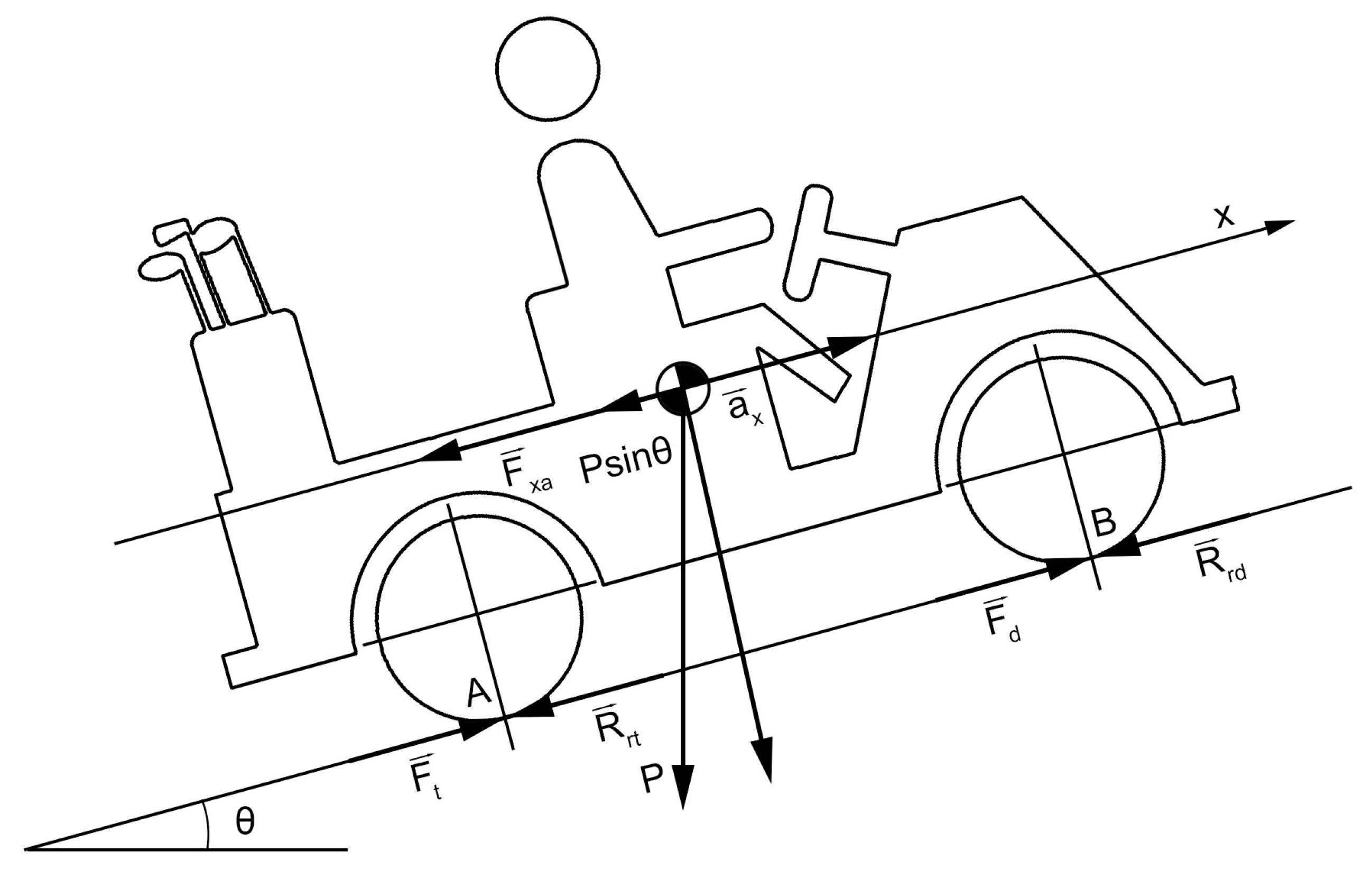
2.1. Design the Traction System

To obtain the energy required for driving the golf car along the predetermined course, we must start with vehicle dynamics and calculate the resistances that oppose movement such as the rolling resistance, aerodynamic resistance, gravitational resistance, and the resistance to inertia, as well as calculating the fundamental equation for the longitudinal movement for these types of forces, where the vertical and pitch forces of sprung mass are ignored. Applying Newton’s second law and the Euler equation we have:

$$m{a}_x=\left(F_t+F_d\right)-R_{rd}-R_{rt}-F_{xa}-P\sin \theta$$

(1)

where

• $m$ = Gross mass and is the sum of m_v + m_BAT + m_PAS + m_BOP + m_H-T + m_equi
• $a_x$ = longitudinal acceleration
• $F_t$ = Front traction effort
• $F_d$ = Rear traction effort
• $R_{rd}$ = Front rolling resistance
• $R_{rt}$ = Rear rolling resistance
• $F_{xa}$ = Aerodynamic drag
• $P$ = Weight of the vehicle, is the product of the mass and gravity
• $\theta$ = Slope angle to be overcome

Figure 5 shows the free solid diagram of the forces that interact with the golf car. We must also consider the inertia caused by the rotating masses of the vehicle (brake discs and drums, transmission system, etc.), which are represented by a factor called mass increase ${\gamma }_m$, and therefore Equation (2) would be as shown below:

$$m{a}_x{\gamma }_m=\left(F_t+F_d\right)-R_{rd}-R_{rt}-F_{xa}-P\sin \theta$$

(2)

$${\gamma }_m=1+{\displaystyle \sum }\frac{I_r}{m{r}^2}+{\displaystyle \sum }\frac{I_t{\mathsf{\xi }}_j^2}{m{r}^2}$$

(3)

where

• ${\gamma }_m$ = Mass factor
• $I_r$ = Moment of inertia of the masses that turn with the wheels with respect to their rotary axes
• $I_t$ = Moment of inertia of the transmission components
• $r$ = kinematic radius equivalent to the radius of the wheel under a load
• ${\mathsf{\xi }}_j$ = Transmission ratio respect to the wheels

While the tractive effort $F_T$ is the sum from front ($F_t$) and rear ($F_d$) traction effort and is defined by:

$$F_T=\frac{M_{ME}{\xi }_d{\xi }_{j^{\prime }}{\eta }_t}{r_c}$$

(4)

where

• $F_T$ = Tractive effort developed by a traction motor on driven wheels
• $M_{ME}$ = Torque of the electric motor
• ${\xi }_d$ = Ratio to the bevel gear
• ${\xi }_{j^{\prime }}$ = Ratio of the gearbox
• ${\eta }_t$ = Efficiency of the transmission
• $r_c$ = Radius under a load

To carry out these calculations, we have considered the weight of the empty golf car and have added the weight of the different components. The battery pack is estimated to weigh 106.4 kg, and the weight of the occupants is estimated for two male adults that are sitting with a weight within the 50th percentile with standing heights of 175 cm and weighing 77 kg each [28], and the weight of the golf clubs is 30 kg each. The values of C_x and f_r are estimated at 0.45 and 0.02, respectively [29].

Table 3. Specifications of golf car.

Specification	Value	Specification	Value
Vehicle mass (mv)	342 kg	Mass factor (γm)	1.042
Battery Pack (mBAT)	106.4 kg	Maximum slope (θ)	25%
Rate load (mPAS)	154 kg	Maximum speed (vmax)	20 km/h
BOP mass (mBOP)	3 kg	Base Speed (Vb)	6 km/h
Mass of the hydrogen fuel tank (mH-T)	6.5 kg	Radius Wheel (re)	0.223m
Mass of golf equipment (mequi)	60 kg	Acceleration time from 0 to 20 km/h (ta)	10 s
Frontal area (Af)	1.72 m2	Drivetrain efficiency (ηj)	99%
Aerodynamic drag coefficient (Cx)	0.45	Ratio of the differential (${\xi }_d$)	12.25
Air density ($\rho$)	1.225 kg/m3	Ratio of the gearbox (${\xi }_{j^{\prime }}$)	1
Gravity acceleration (g)	9.81 m/s2	Maximum efficiency of the E.M (ηME)	92%
Rolling resistance coefficient (fr)	0.02	Efficiency of the DC-DC converter (ηDC-DC)	90%

lists all the parameters that have been considered.

2.1.1. Golf Car Performance Criteria

The performance of the proposed vehicle is detailed below based on the standard for this type of vehicle. The design is related to the vehicle’s response during longitudinal movements. Three determining criteria are taken into account, which include the following: the maximum speed, acceleration, and maximum slope. Based on these it calculates the propulsion power required for moving the vehicle [26,30].

Power Required for Reaching Maximum Speed

The traction power required for reaching maximum speed can be obtained using the following expression:

$$P_{t_{vel}}=\left[\left(mg{f}_r\right)+\left(\frac{1}{2}\rho C_x{A}_f{v}_{max}^2\right)\right]v_{max}$$

(5)

where

• $P_{t_{vel}}$ = Power rating for reaching maximum speed
• $g$ = Gravity
• $f_r$ = Rolling resistance coefficient
• $C_x$ = Aerodynamic drag coefficient
• $\rho$ = Air density
• $A_f$ = Frontal area
• $v_{max}$ = Maximum speed

The maximum speed is determined based on the performance we wish to obtain for a vehicle intended to be used to drive around a golf course. According to standard ANSI/ILTVA Z130.1-2012, it must not exceed 24 km/h, nor shall it be able to accelerate 0.5 g (4.9 m/s²) for intervals exceeding 0.2 s [31]. For this vehicle, the maximum speed is set at 20 km/h.

Power Required for Acceleration

To assess these criteria, we have considered the behavior of the vehicle on a flat track and then evaluated the behavior of the vehicle when transitioning from low speed (0 km/h) to high or maximum speed (20 km/h). In this case, we must calculate the time and distance required to reach this speed. Since this is an electric vehicle, the test is conducted at maximum torque, since in electric motors, the torque is a simple function of the speed. At low speeds, the torque is normally constant until reaching a base speed, and after this, the torque decreases. The acceleration time can be determined using the following expression:

$$\begin{array}{cc}{t}_a=& {{\displaystyle \int }}_0^{V_b}\frac{m{\gamma }_m}{\frac{P_{ME,max}{\eta }_t}{V_b}-mg{f}_r-\frac{1}{2}\rho C_x{A}_f{V}^2}\mathrm{d}v\\ & +{{\displaystyle \int }}_{V_b}^{V_f}\frac{m{\gamma }_m}{\frac{P_{ME,max}{\eta }_t}{V}-mg{f}_r-\frac{1}{2}{\rho }_a{C}_x{A}_f{V}^2}\mathrm{d}v\end{array}$$

(6)

where

• $P_{ME,max}$ = Maximum Power of the electric motor
• $V_b$ = Base Speed
• V = Vehicle Speed

The first term on the right-hand side of Equation (6) is in correspondence with the speed region lower than the vehicle base speed, and the second term is in correspondence with the speed region beyond the vehicle base speed. However, we can obtain an approximation, i.e., decreasing the rolling and aerodynamic resistance. This way the traction power is determined by the following expression:

$$t_a=\frac{m{\gamma }_m}{2P_{t_1}}\left(V_f^2-V_b^2\right)$$

(7)

$$P_{t_{ac{e}^{\prime }}}=\frac{m{\gamma }_m}{2t_a}\left(V_f^2-V_b^2\right)$$

(8)

where

• $t_a=$ Acceleration time from 0 to 20 km/h
• $V_f$ = Final Speed
• $P_{t_{ac{e}^{\prime }}}$ = Power consumed for vehicle acceleration

The equation above does not include the average drag power during acceleration ($\overline{P}{\_}_{drag}$), which can be defined as:

$$\overline{P}{\_}_{drag}=\frac{1}{t_a}{{\displaystyle \int }}_0^{t_a}\left(mg{f}_{r}V+\frac{1}{2}\rho C_x{A}_f{V}^3\right)\mathrm{d}t$$

(9)

$$V=V_f\sqrt{\frac{t}{t_a}}$$

(10)

$$\overline{P}{\_}_{drag}=\frac{2}{3}mg{f}_r{v}_f+\frac{1}{5}{\rho }_a{C}_x{A}_f{V}_f^3$$

(11)

Adding the average drag power to the traction power of Equation (8), the traction power in acceleration would be expressed as:

$$P_{t_{ace}}=\frac{{\gamma }_{m}m}{2t_a}\left(V_f^2+V_b^2\right)+\frac{2}{3}mg{f}_r{V}_f+\frac{1}{5}{\rho }_a{C}_x{A}_f{V}_f^3$$

(12)

The power required for acceleration ($P_{t_{ace}}$) in this equation is applied to a specific acceleration standard where $t_a$ is the acceleration time employed, which in this case is 10 s, as it is defined based on how long it takes the vehicle to reach its maximum speed from its initial speed equal to 0 km/h, $V_b$ is the base speed of the vehicle (6 km/h), $V_f$ is the final and maximum speed (20 km/h) speed of the vehicle.

Traction Power Required for the Maximum Slope

In this section, we analyze the traction power required for the vehicle to overcome the maximum slope (25% for paved roads and 15% for unpaved roads [28]), at a certain speed (6 km/h). Given that the analysis is carried out on a steep slope and at a low speed, the aerodynamic resistance can be decreased and therefore it can be determined using the following expression:

$$P_{t_{slp}}=\left(mg{f}_r+mg\sin \theta \right)V_b$$

(13)

where θ is the angle of the slope to be overcome and $V_b$ is the speed it must travel to overcome the slope (Base Speed in this application). The results show that the traction power required for maximum speed ($P_{t_{vel}}$) is equal to 0.82 kW for an acceleration ($P_{t_{ace}}$) of 1.62 kW and for a maximum slope ($P_{t_{slp}}$) of 2.42 kW, therefore applying the three criteria. Then as a minimum, the power rating ($P_t$) of the electric motor must have the power obtained for maximum slope.

Torque Required by the Electric Motor

The maximum motor torque characteristic is described via the correlations between the output torque, the output power, and the angular speed. The electric motor torque is calculated using the following expression:

$$M_{ME}=\frac{P_{ME}}{{\omega }_{ME}}$$

(14)

Likewise, for the wheel:

$$M_{ME}=\frac{M_{re}}{{\xi }_j}$$

(15)

where

• $M_{ME}$ = Output torque
• $P_{ME}$ = Output power
• ${\omega }_{ME}$ = Angular speed
• $M_{re}$ = Torque on the wheel
• ${\xi }_j$ = Final transmission ratio

${\xi }_j$ is equal to the transmission ratio of the differential (${\xi }_d$ = 12.25) since it does not have a gearbox (${\xi }_{j^{\prime }}$ = 1). Using these expressions, we can determine that the required torque on the wheels is 445.25 Nm and the minimum motor torque is 36.34 Nm at a minimum power of 2.42 kW. The characteristics of the selected motor are described in

Table 4. Electric Motor HPEVS AC-20 specifications.

Specification	Values
Drive Motor	48 VDC, 3 kW @ 3000 rpm
Peak Power	7.82 kW @ 1248 rpm
Torque	10.4 Nm @ 3000 rpm (Nominal Torque) 40.71 Nm @ 1248 rpm (Maximum Torque)
Batteries	Four 12 V, 77 min @ 56 A

.

Determining the Size of the Batteries

For determining the size of the batteries, we have estimated the instant traction power required by the golf car at each one of the sections of the circuit. Additionally, we have calculated the energy consumption accumulated in each section in order to be able to estimate the characteristics of the energy storage system (Figure 6a,b). A preliminary design can be estimated using the following expressions:

$$E_{BES}=\frac{\Delta E_{max}}{SO{C}_t-SO{C}_b}$$

(16)

$$C_{BAT}=\frac{E_{BES}}{V_{DC}}{\eta }_{BAT}f$$

(17)

where

• $E_{BES}$ = Energy of the vehicle’s storage system
• $\Delta E_{max}$ = Energy consumed during the cycle
• $SO{C}_t$ = Top state of charge
• $SO{C}_b$ = Bottom Minimum state of charge
• $C_{BAT}$ = Capacity of batteries
• $V_{DC}$ = Nominal voltage of the system
• ${\eta }_{BAT}$ = Battery efficiency
• $f$ = Charge factor

It must be taken into account that the lead acid batteries must not be discharged beyond 10.5 V (for a 12 V battery) at a temperature of 25 °C [32]. $\Delta E_{max}$ is the energy consumed during route 1 and 2. Based on the state of the charge curve, we have considered a $SO{C}_t$ of 30% and $SO{C}_b$ equal to 90%, which are representative values that guarantee a high number of charge and discharge cycles for this type of battery, the state of charge introduced in expression (16) is 60% and it is the variation of SOC (ΔSOC). ${\eta }_{BAT}$ is the battery’s efficiency equal to 85% [33] and $f$ is the charge factor that guarantees obtaining the battery capacity at 1C and is equal to 1.5. The energy obtained by the storage system is 1205 Wh for the entire circuit and the capacity of the batteries is 32 Ah. The values obtained using these equations are considered referential because they belong to a static cycle where an average power is considered. For a dynamic cycle, we must consider relevant factors such as the required power peaks, which may affect the service life of the batteries in addition to the Peuker effect (relationship between the state of charge of a battery and its discharge ratio). A more conservative approximation consists of evaluating the recurrence with which each instant power value is required and classifying it statistically, as shown in Figure 7. Analyzing the power peaks listed in Figure 6a,b, we see values up to 10 kW. However, if we look at the frequency of the demand for each power value throughout the course, we can determine that the instant traction power does not exceed 5000 W approximately 95% of the time in both routes, and therefore, a more rugged design from an energy perspective is to consider using four 12 V batteries connected in series and with a capacity of 105 Ah. We have evaluated and characterized five types of batteries, two with a capacity of 155 Ah, one with 115 Ah, and two with 105 Ah. The batteries selected based on their performance are US 27DC XC 2 and their specifications are shown in Table 4. We considered optimal this selection for this application and typology. Since a pack of batteries of greater capacity would be overestimated in addition to the inconvenience of increasing the weight of the vehicle and a pack of smaller batteries would not cover the demand in power peaks.

State of Charge of Batteries

The state of charge refers to the current capacity of a battery and is defined as the ratio of the available capacity Q_QH to the nominal capacity Q_QH,max.

$$\mathrm{SOC}=\frac{Q_{QH}}{Q_{QH,max}}$$

(18)

In a time interval $dt$ with a constant discharge current $i$, the state of charge can be expressed by the current integration method as:

$$\mathrm{SOC}=\frac{Q_{QH,max}-{{\displaystyle \int }}_{t_0}^{t}i dt}{Q_{QH,max}}$$

(19)

The estimation of the state of charge is a fundamental parameter in vehicles of this type. The methods commonly used to estimate the SOC are the following: the Coulomb counting approach, open-circuit voltage measurements, dynamic equivalent circuit-based models, electrochemical impedance spectroscopy, the artificial neural network approach, and extended Kalman filters (EKFs). The physical model of the present work estimates the state of charge by means of the Coulomb Counting method, which is a suitable method used in electric vehicles, which consists of calculating the SOC by measuring the current of the battery and integrating it over time, it is a very simple method but has to start from a correct load value [34].

If we consider in the model of Equation (19) parameters expressed in Wh, the voltage V(t) is related to the current i(t), the state of charge can be expressed [35,36]:

For mode EV:

$$SOC=1-{{\displaystyle \int }}_{t_0}^t\left(W_{dis}-W_{chg}\right)\mathrm{d}t/E_{batt}$$

(20)

while for mode FCEREV:

$$SOC=1-{{\displaystyle \int }}_{t_0}^t\left(W_{dis}-W_{chg}-W_{FC}\right)\mathrm{d}t/E_{batt}$$

(21)

where

• $SOC$ = State of charge
• $W_{dis}$ = battery discharge power
• $W_{chg}$ = battery charge power from regenerated kinetic energy
• $W_{FC}$ = battery charge power from Fuel cell system
• $E_{batt}$ = battery’s energy storage capacity, which is obtained by the multiplication of the capacity of the battery and the nominal voltage.

2.2. Energy Management Proposal with Fuel Cell

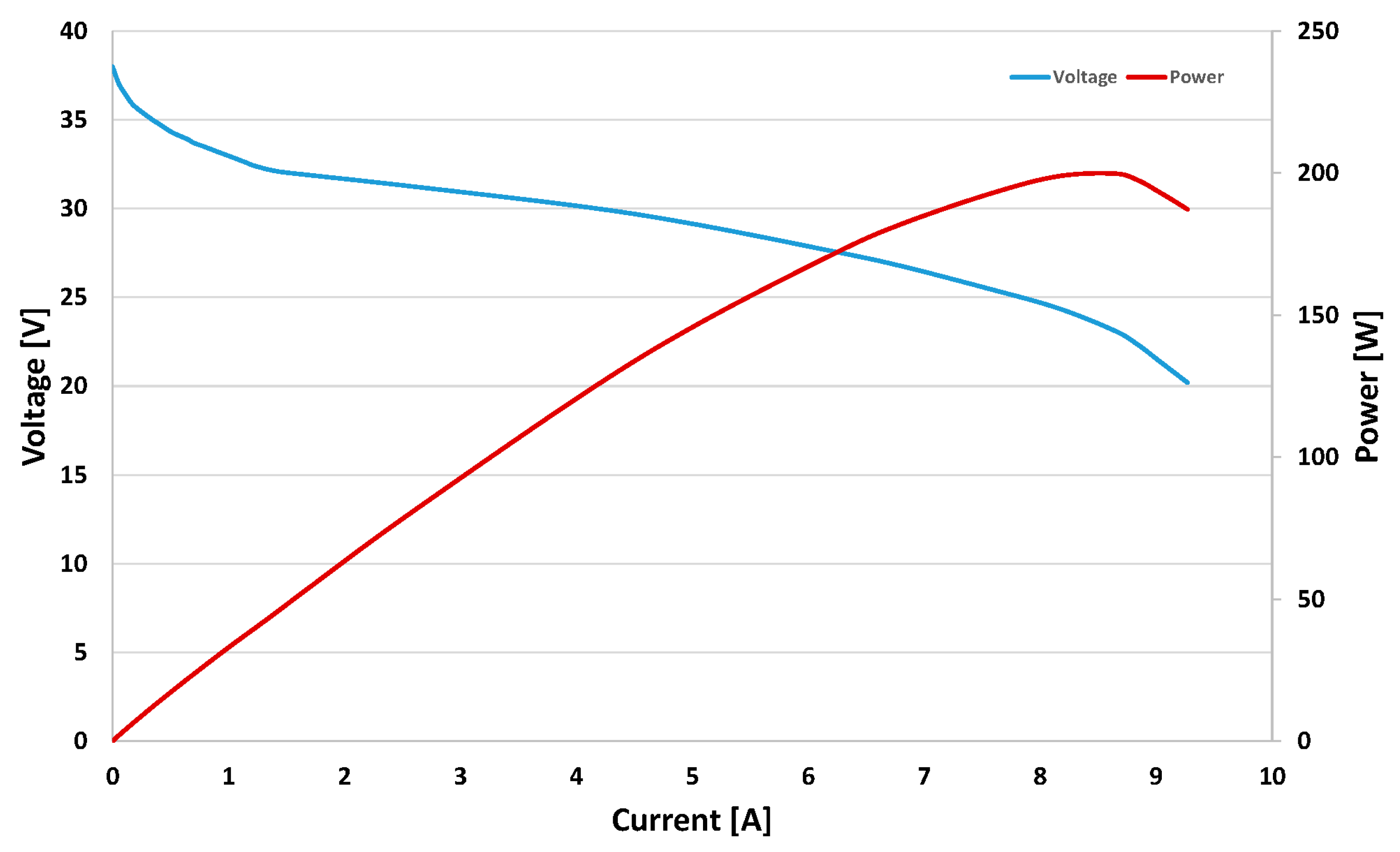
Once the size of the components of the powertrain and its main power source have been determined, a 200 W fuel cell is added to the system. The function of this component is to charge the battery pack throughout the entire course, and its small size is sufficient to meet the energy requirements of this analysis since this is an auxiliary energy system. This way, the golf car will be an electric vehicle with an extended range or a hybrid vehicle in series. The purpose of this configuration is to allow making several trips throughout the day without needing to charge the battery by connecting the vehicle to the electrical power grid. Charging is usually carried out at night and, this way, the vehicle is only limited by the autonomy provided by its batteries.

The fuel cell that is used is made of polymer electrolyte membrane (PEM), specifically from the Horizon FCS-C200 brand (from Horizon Fuel Cell Technologies, Singapore). Its characteristic parameters are listed in

Table 5. Fuel Cell FCS-C200 specifications [37,38].

Specification	Value	Specification	Value
Number of cells	40	Max stack temperature	65 (°C)
Cell active area	19 (cm2)	H2 Pressure	0.45–0.55 (bar)
Current density	0.437 (A·cm−2)	Hydrogen purity	≥99.995 H2
Rated Power	200 (W)	Efficiency of stack	40% @ 24 V
Voltage in the maximum power point	24 (V)	Flow rate at max output	2.6 (L/min)
Current in the maximum power point	8.3 (A)	Stack weight (with fan, casing and Controller)	2.63 (kg)
Open circuit voltage (VOC)	38 (V)	Size	11.8 × 18.3 × 9.4 (cm)

.

The fuel cell’s polarisation and power curve are provided in Figure 8, where the electric power in an open circuit is 0.95 V, which is less than the theoretical 1.23 V per cell. We can also see that at high voltages, the current supply is low and, therefore, the behavior of the cell at this point is not ideal. In this region there are primarily power losses in the cathode catalyst layer (CCL) called oxygen reduction reaction (ORR). Having passed this zone, the curve stabilizes and the voltage drop is nearly linear, and the losses that predominate here are resistive and ohmic. Finally, at low voltages (lower than 0.6 V per cell), the current drops sharply and, therefore, the power drops as well. In this area, the losses that predominate are due to the transport of masses of the cathode catalyst layer CCL and the gas diffusion layer GDL [39].

Fuel Cell Model

The following expression defines the voltage of each fuel cell with the different losses it is exposed to:

$$Vcell=V_{OC}-{\eta }_0-R_{\Omega }{j}_0$$

(22)

where V_OC is the open circuit voltage (0.95 V in this case); $R_{\Omega }{j}_0$ is the ohmic loss resulting from the ionic resistance in the electrolyte, the electrodes, the electronic resistance of the electrodes, collectors and the contact resistance; η₀ is the total voltage loss in the cathode catalyst layer (CCL) and are represented by the following expression [37,38,39,40]:

$${\eta }_0=act+t_{CCL}+t_{GDL}$$

(23)

The activation losses are defined as:

$$act=b\arcsin h\left(\frac{{\left(\frac{j_0}{j_{\sigma }}\right)}^2}{2\frac{c_h}{c_{ref}}\left(1-\exp \left(\frac{-j_0}{2j_{*}}\right)\right)}\right)$$

(24)

where b is the Tafel slope, its value is normally 0.03 V; j₀ is the density of the current in the cell 0.437 A·cm⁻²; j_σ is a current density parameter (j_σ = 2i_∗σ_tb); $c_h$ is the molar concentration of oxygen in the channel; $c_{ref}$ is the molar concentration of reference; and $j_{*}$ is a scalar parameter of current density ($j_{*}=\frac{{\sigma }_{t}b}{l_t}$).

The loss due to the transport of mass in the CCL is equal to:

$$t_{CCL}=\frac{\frac{{\sigma }_t{b}^2}{4FD{c}_h}\left(\frac{j_0}{j_{*}}-\ln \left(1+\frac{j_0^2}{j_{*}^2{\beta }^2}\right)\right)}{1-\frac{j_0}{j_{lim}^{*}\frac{c_h}{c_{ref}}}}$$

(25)

where σ_t is the ionic conductivity in the CCL; F is the Faraday constant; D is the oxygen diffusion coefficient in the CCL; and β is a dimensionless parameter based on the value of the dimensionless current density ${\tilde{j}}_0$ that is related with the polarisation curve of the cell, where its value is usually within a transition speed of ≅1 for PEM cells [40] ($\beta =\frac{\sqrt{2{\tilde{j}}_0}}{1+\sqrt{1.12{\tilde{j}}_0}exp\sqrt{2{\tilde{j}}_0}}+\frac{\pi {\tilde{j}}_0}{2+{\tilde{j}}_0}$); and $j_{lim}^{*}$ is the current density limit resulting from the transport of oxygen in the GDL ($j_{lim}^{*}=\frac{4F{D}_b{C}_h^{*}}{l_b}$).

Finally, the loss due to the transport of mass in the GDL is equal to:

$$t_{GDL}=-b\ln \left(1-\frac{j_0}{j_{lim}^{*}\frac{c_h}{c_{ref}}}\right)$$

(26)

The values of these parameters are listed in

Table 6. Specifications for the polarization curve in the automotive software simulator [37,38,39,40].

Specification	Value	Specification	Value
Open circuit voltage (VOC)	0.95 (V)	Cell current density (j0)	0.437 (A·cm−2)
Tafel slope (b)	0.03 (V)	Faraday constant (F)	96,485 (As·mol−1)
Current density parameter (jσ)	1.212 × 10−3 (A·cm−2)	Oxygen diffusion coefficient in the CCL ($D$)	1.36 × 10−4 (cm2·s−1)
Scalar parameter of current density ($j_{*}$)	0.9 (A·cm−2)	Dimensionless parameter ($\beta$)	1311
Volumetric exchange current density (i∗)	8.17 × 10−4 (A·cm−3)	Limiting current density due to oxygen transport in the GDL ($j_{lim}^{*}$)	2958 (A·cm−2)
Catalyst layer thickness $(l_t)$	0.001 (cm)	Oxygen diffusion coefficient in the GDL ($D_b$)	0.0259 (cm2·s−1)
Oxygen concentration in the channel ($c_h$)	7.4 × 10−6 (mol·cm−3)	Ohmic Resistance	0.126 (Ω·cm−2)
Oxygen concentration at the channel inlet ($C_h^{*}$)	7.36 × 10−6 (mol·cm−3)	GDL thickness ($l_b$)	0.025 (cm)
Reference oxygen molar concentration ($c_{ref}$)	7.36 × 10−6 (mol·cm−3)	Dimensionless current density (${\tilde{j}}_0$)	1
CCL ionic conductivity (σt)	0.03 (S/cm)	Limiting current density due to oxygen transport in the GDL ($j_{lim}^{*}$)	2.95 (A·cm−2)

.

2.3. Efficiency of the System

The calculation of the total efficiency for a FCHEV vehicle is the same for the configuration battery/fuel cell as fuel cell/battery, this is because in both cases there is strictly an electrical coupling, unlike conventional hybrid vehicles that can also have mechanical couplings, however, the performance may vary according to the operating conditions and the control strategy taken. The following expression defines this set up well:

$${\eta }_T={\eta }_{FC} {\eta }_{DC-DC} {\eta }_{BAT} {\eta }_{ME} {\eta }_j$$

(27)

where

• ${\eta }_T$ = Total efficiency
• ${\eta }_{FC}$ = Fuel cell System efficiency
• ${\eta }_{DC-DC}$ = Efficiency of the DC-DC converter
• ${\eta }_{BAT}$ = Battery efficiency
• ${\eta }_{ME}$ = Efficiency of electric machine
• ${\eta }_j$ = Drivetrain efficiency

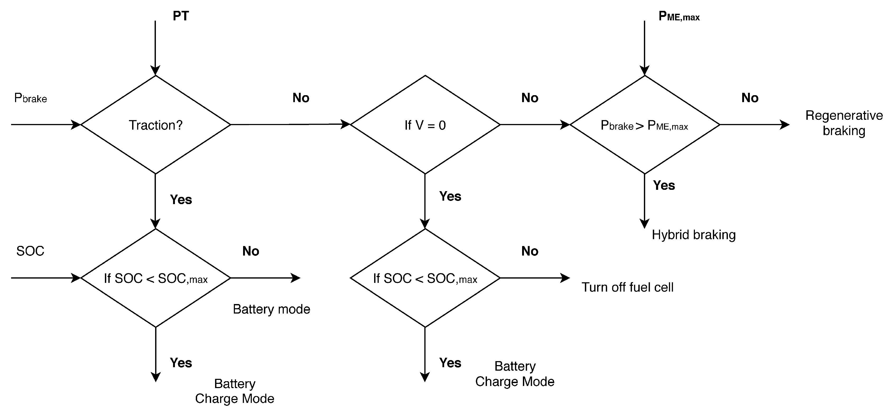
2.4. Control Strategy—Max. SOC of Battery

The desired objectives in this application include the following: the satisfaction of the power demanded by the driver, optimal performance of the components of the hybrid system, and above all to keep the SOC as high as possible at the end of each game of golf. The FCEREV configuration we have considered optimal for this application because its requirements are not as high as in a light-duty vehicle where a fuel cell/battery configuration is adequate. Figure 9 shows the control strategy adopted in the model, showing how to ensure a high behavior of the vehicle at any time. The batteries are the main source of energy and those that cover the peaks of power, while the fuel cell is an auxiliary component that minimally contributes to traction, and its main objective is to charge the battery. This strategy is suitable for applications in which the behavior (speed, accelerations, slopes, etc.) is the first concern, such as vehicles with frequent stops and starts [41].

3. Results and Discussion

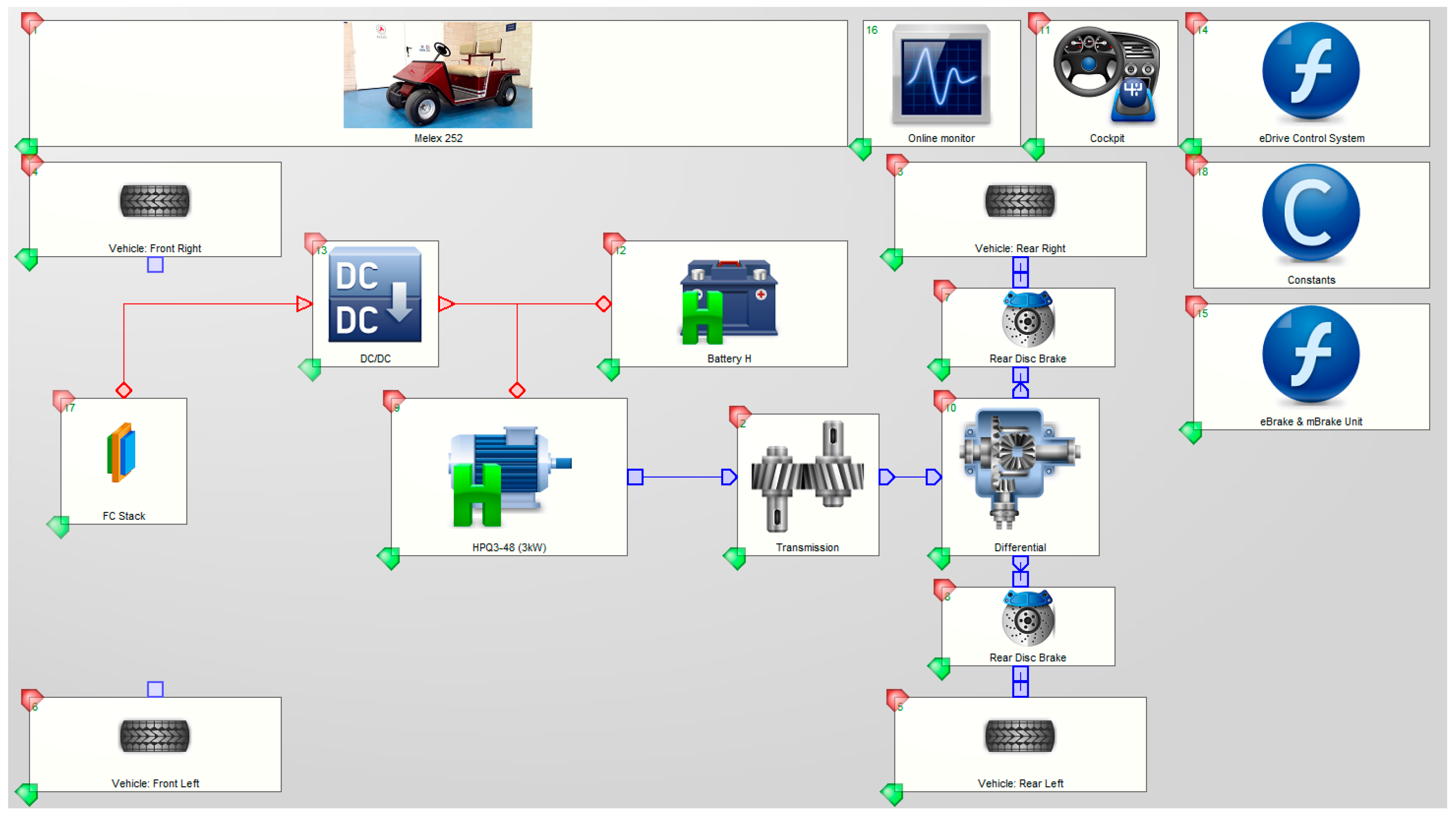
3.1. The Simulation Tool

The game of golf entails making stops between holes, and also at each hole, the players may have to take several swings or shots that entail more stops. We estimate that each stop of the vehicle will take 180 s, and therefore, on average, a full game of golf could take about 195 min. The previously exposed speed profiles have been treated based on this assertion and new speed profiles have been determined for Section 1 and Section 2 as seen in Figure 10a,b, which include stops during the game. Since the fuel cell is small size, it will be operating at all times. When the vehicle is being driven, the fuel cell will provide power for the electric motor and when the vehicle is stopped, it is used to charge the batteries. At the end of the day, two objectives must be achieved: the first is to make more trips than an EV golf car and the second is to finish the day with a state of charge above 30%.

The simulation of the system has been carried out using the AVL CRUISE software (Version 2017, AVL, Graz, Austria) [42]. This simulation tool allows conducting the energy analysis and optimization of motor vehicles with conventional, hybrid, and electric powertrains. Its focus is on fuel efficiency, emissions, and the analysis of the performance throughout the vehicle development process. The model that was made is shown in Figure 11, which includes several blocks connected to each other, and based on a logic algorithm, they are predefined to interact with each other. Block 1 shows the model vehicle. Block 2 is the final drive, and this block makes a reference to the final transmission of the vehicle. Blocks 3 to 6 are the tires that connect the vehicle to the road. Blocks 7 and 8 are the vehicle’s brakes. The brakes are described using braking data and sizes as well as a specific braking factor. Block 9 is the eDrive HPQ3-48 (from Hepu Power Technology Co., Zhaoqing, Guangdong, China) and represents the electric drive machine. It may operate as a motor or generator and is defined based on its characteristic map. The block includes the DC-AC converter. Block 10 references the gear and differential. Block 11 is the cockpit, and the function of this component is to connect the driver with the vehicle and the connections are made through the data bus. Block 12 refers to the drive batteries. The basic model consists of a voltage source and an ohmic resistance. The resistance model is designed to take into account a large number of the complex processes occurring inside the battery. Block 13 corresponds to the DC-DC converter. This component is used to efficiently transform DC voltages, its function is to couple the different voltage ranges to that which is suitable for the electric motor, which allows for a proper energy flow between the components involved in the current bus. Block 14 corresponds to the e-Drive Control System function and block 15 to the eBrake and mBrake Unit. Their functions are defined by the user and they are programmed in the C programming language. The eDrive function corresponds to the control of the electric motor and the eBrake function to the regenerative braking function.

Block 16 corresponds to the monitor. This component allows displaying some results of the calculation while the simulation is being executed. Block 17 corresponds to the proton exchange membrane fuel cell (PEMFC). The model is based on the electro-chemical equations that are analyzed (Equations (21)–(25)). These equations are derived from the polarization curve of the cathode side and take into account the activation, ohmic, and mass transport losses. Finally, block 18 defines constant values, which may be used by other blocks via the data bus.

3.2. Model Simulation and Validation

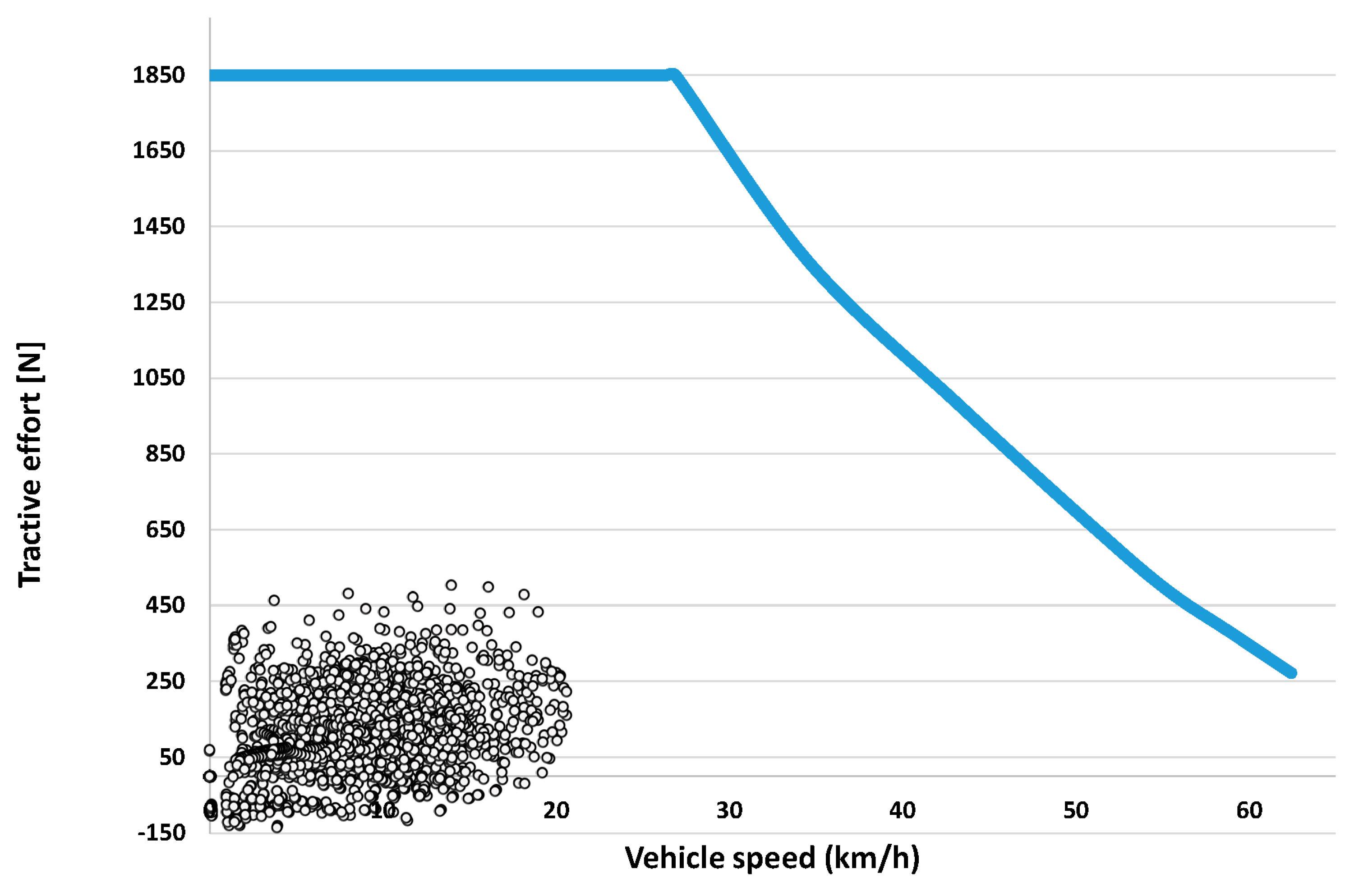
3.2.1. Tractive Effort throughout the Course

A proper design of the drive system must guarantee that the tractive effort throughout the course at the destination speed range does not exceed the maximum tractive effort (calculated using expression (4)). Based on the speed profile obtained at a golf course, the maximum capacities are rarely used. In fact, most of the time, the drive system is operating at partial load as we can see in Figure 12. In a large measure, the operating range depends on the operating conditions such as accelerations, decelerations, and climbing up or going down slopes. However, the obtained speed profile can be assumed as the typical behavior of a driver on a golf course, and therefore, the sizing of the electric motor meets the different range of demands. It is worth mentioning that since the electric motor operates in several angular speed ranges and under different conditions, its efficiency differs from the maximum. To obtain more reliable results, a test has been conducted on a test bench of the motor torque and efficiency curve based on the speed. This is shown in Figure 13.

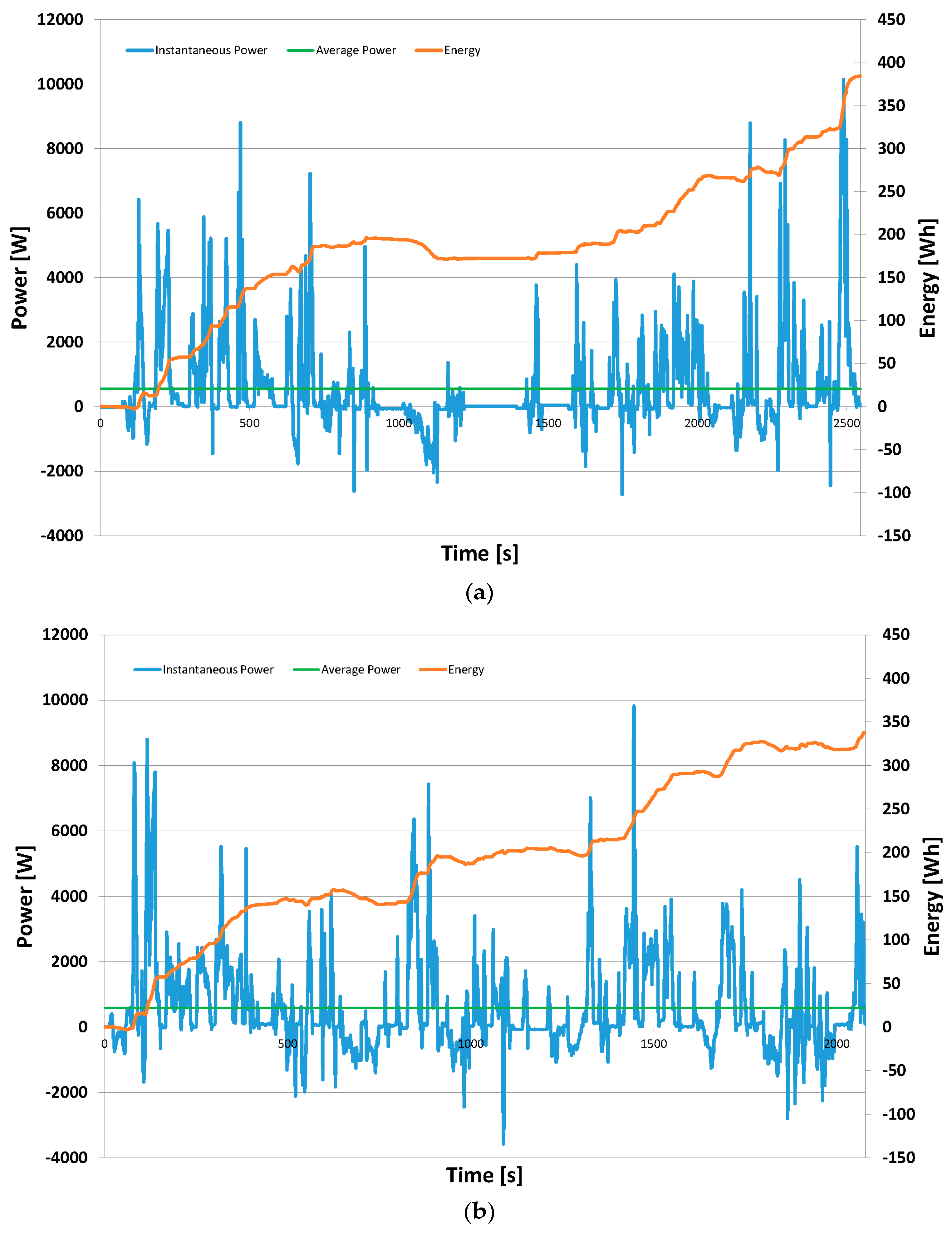
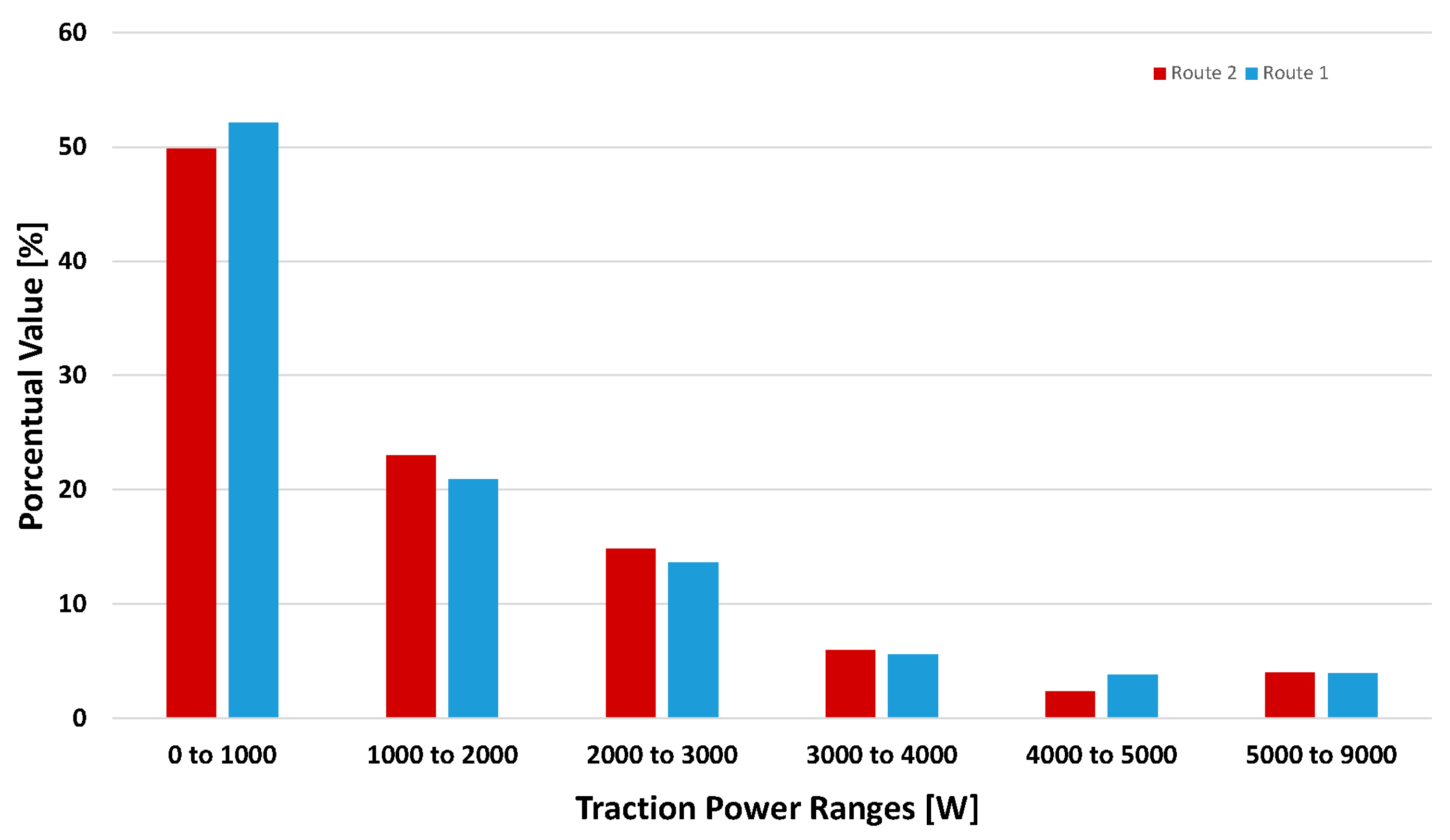
3.2.2. Managing the Power and Energy of the Drive System

We have conducted a simulation of the behavior of the golf car based on the speed profile of Figure 14, which is the connection between route 1 and 2.

The demand for power from the electric motor (Figure 15) is in a large measure covered by the batteries, and their state of charge will depend on the operating conditions. Figure 16 shows the power supplied by the battery pack on the circuit. Peaks nearing 6 kW are experienced during the most demanding conditions and we also see that during the tests, the average power of the fuel cell is 160 W. The function of this element is to provide its energy throughout the course. In fact, based on an initial SOC of 90% that is assumed at the start of the day, the cell never stops operating in a constant mode, and this is because its power is small and its main function is to charge the batteries in order to maintain a high SOC at the end of the day.

Figure 17 shows the total electric power consumption during the course. The balance shows that a total energy of 0.597 kWh (Total Output Energy) was consumed during the driving cycle, of which 0.168 kWh (Energy discharge) was provided by the battery, 0.079 kWh by the regenerative braking, and 0.350 kWh (Total Input Energy) by the fuel cell.

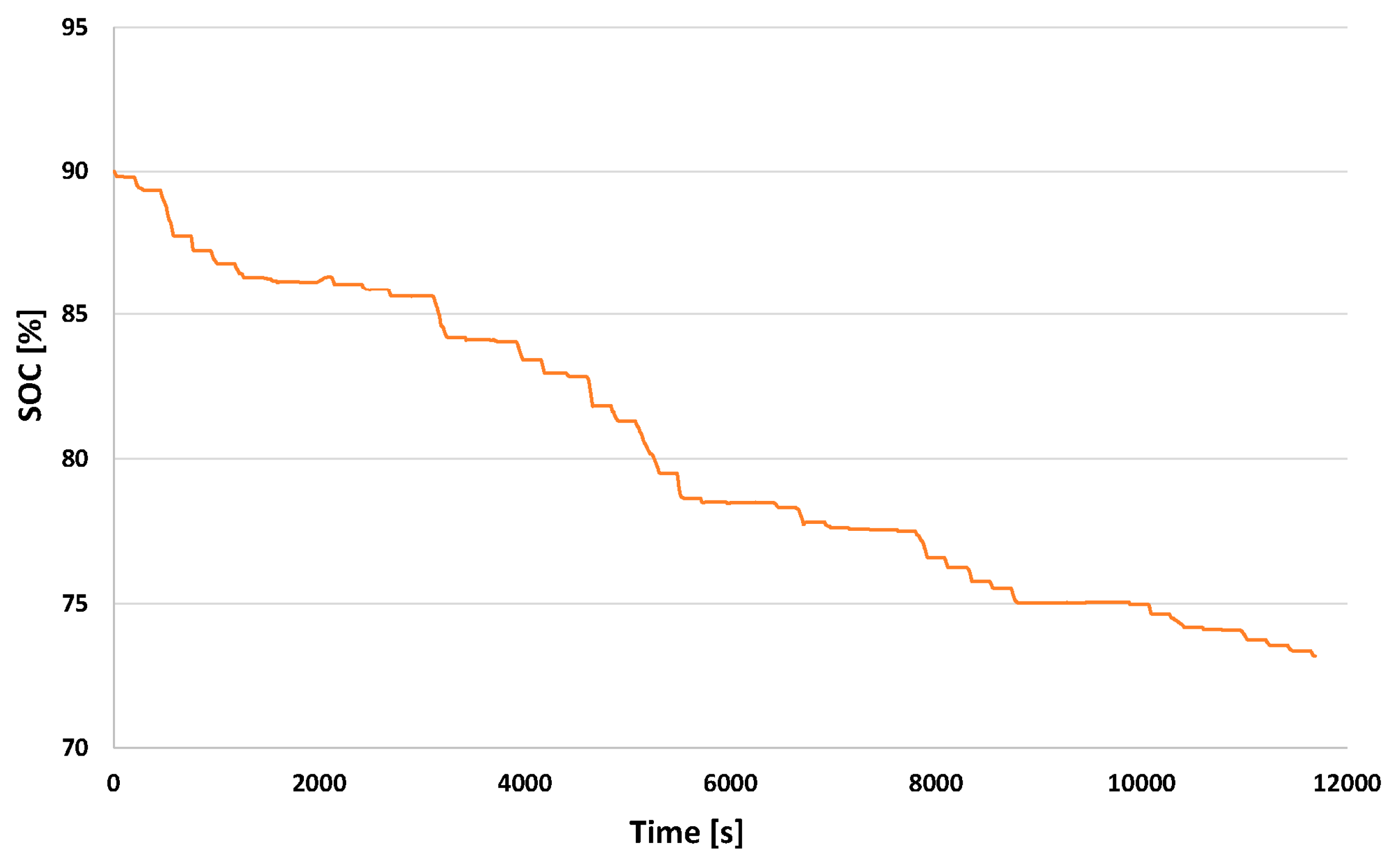
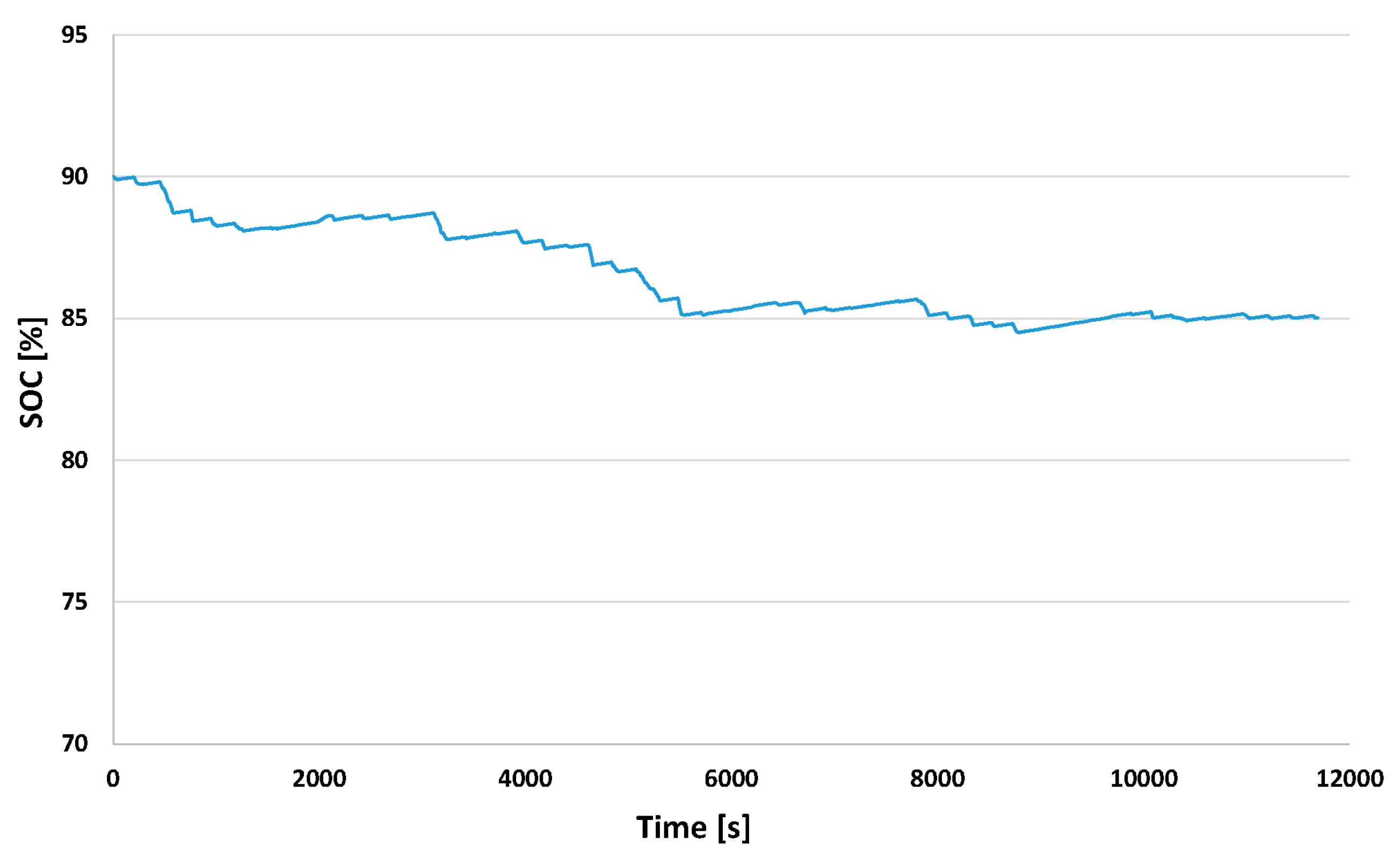
3.2.3. State of Charge in EV and in FCEREV

From the simulation made for the complete circuit, Figure 18 shows the results of the state of charge for the electric mode and Figure 19 shows the state of charge for the electric mode with fuel cell. After travelling 8 km, the state of charge in EV mode went from an initial SOC of 90% to a final SOC of 73.17%, or in other words, a decrease of 16.83%, unlike the FCEREV mode where the state of charge at the end of the course was 85.0%, with a decrease of only 5.0% from the initial.

These results are favorable and the aim of this arrangement is to extend the autonomy of the vehicle so that it can make the highest number of trips in a day. The purpose is to have an SOC of no less than 30% at the end of the day, which would shorten the life of the batteries as well as not having the vehicle available for the rest of the day. The analysis is especially set during the summer, where the courses can begin at 07:00 and end at 12:00, which would require making at least five trips. In electric mode, the vehicle could not make more than three trips since it would end up with an SOC of 39.51% and this would not allow making a fourth trip. However, since the vehicle incorporates a small sized fuel cell, the autonomy can be extended and two more trips can be made without needing to charge the vehicle.

The hydrogen that supplies power to the fuel cell is stored in metallic hydrides, the capacity of the bottle is 2400 cm³, it weighs 6.5 kg, and contains 0.085 kg H₂, which allows extending the autonomy by 11.7 km as compared to the electric mode, with the battery ending up with a state of charge of 65% after having made five trips.

Table 7. Comparison of FCEREV vs. EV.

Parameter	Mode EV	Mode ERFCEV	Difference
Autonomy (km)	30.8	42.5	11.7
H2 Consumption (kg/100 km)	-	0.200	-
Chargeini (Ah)	94.5	94.5	-
Chargefin a (Ah)	76.83	89.26	12.43
SOCini (%)	90.0	90.0	-
SOCfin a (%)	73.17	85.0	11.83
SOCfin b (%)	56.34	80.0	23.66
SOCfin c (%)	39.51	75.0	35.49

^a After one trip around the golf course; ^b After two trips around the golf course; ^c After three trips around the golf course.

shows the relevant results of this analysis.

3.2.4. Comparative Analysis with Others Battery Technologies

The technology of the batteries is diverse. In the present, there are old technologies that have consolidated until new technologies arise with greater densities of power and more outstanding power. Next, the main batteries that are used in the automotive sector for propulsion of a vehicle are detailed. The lead acid batteries have an energy density between 20 and 50 Wh/kg [43,44], and their advantage lies in being a known and mature technology. Thus, their cost is approximately 100 USD/kWh, although the energy density is low but appropriate for vehicles with low performance [45]. Ni-MH batteries are used in hybrid vehicles such as the Toyota Prius, and its energy density is 60 to 80 Wh/kg [45], while its cost is estimated between 700 and 800 USD/kWh [44]. It is a mature technology, but it has already reached its highest potential, both in cost reduction and in characteristics. The lithium-ion battery has gained much acceptance in the automotive industry due to its excellent characteristics, and it is planned as the technology to adopt in propulsion systems of hybrid and electric vehicles. Its energy density varies between 80 and 120 Wh/kg and its price can be around 750 USD/kWh [45]. Finally, sodium nickel chloride batteries (Na/NiCl₂, Zebra) are a safe and low-cost technology (one third of the price of lithium-ion batteries) and also has a satisfactory energy density that is comparable to that of Li-ion (approximately 120 Wh/kg). Its disadvantage is that its specific power is much lower (150 W/kg), which causes a greater weight in a vehicle per unit of power [46].

Table 8. Comparisons between different battery technologies applied to the simulation of golf car.

Battery Technologies	Energy Density (Wh/kg)	Implementation Technology Cost ($)	Total Output Energy (kWh)	ΔE (%)	SOC (%)	ΔSOC (%)
Lead acid battery	47.3	504	0.597	0	85.0	0
Nickel Metal Hydride battery (Ni-MH)	70.0	3528	0.5829	−2.36	85.67	0.79
Lithium-ion battery (Li-Ion)	100	3780	0.5722	−4.15	85.78	0.92
Sodium Nickel Chloride (Na/NiCl2, Zebra) battery	100	3780	0,6539	9.53	84.71	−0.58

shows comparisons acquired through a series of simulations applied to a golf car between the different battery technologies. The total energy output and SOC have been obtained for each type of battery and ΔE and ΔSOC is the variation of energy and SOC, respectively, of the batteries of lead acid compared to the rest of the technologies. As can be seen, the least efficient technology is that of lead batteries, however their costs are much lower than the rest of the technologies, so for applications of this type, they are the most suitable.

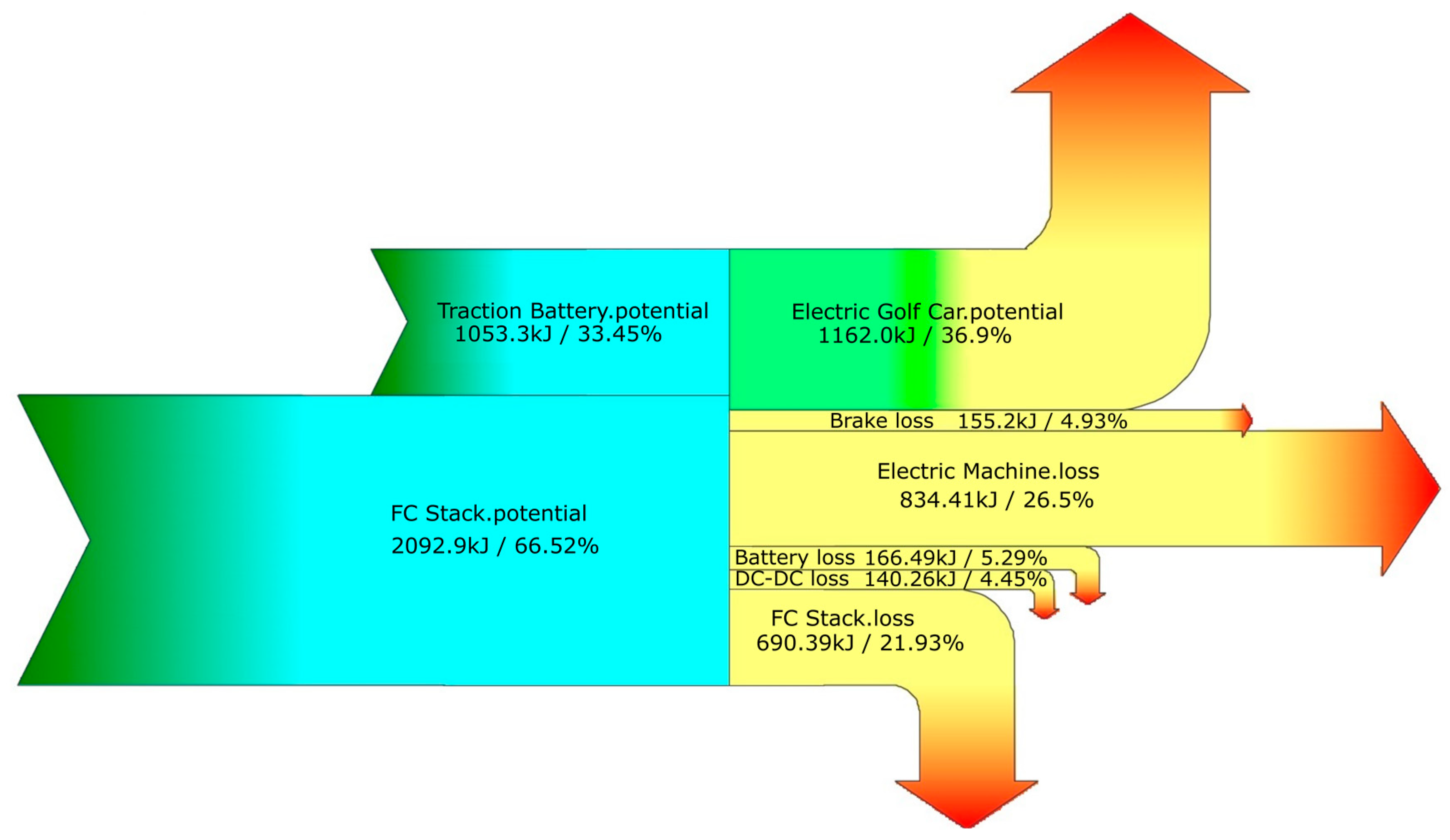
3.2.5. Sankey Energy Diagram during the Trip

Like all energy systems, this system also loses energy during the energy conversion process. Figure 20 shows the Sankey diagram that explains this loss. The input energy is supplied by two sources: the traction batteries and the fuel cell system. With this design, the batteries are the main source while the fuel cell is an auxiliary system that supplies constant energy for charging the batteries and supplying the electric motor, depending on the situation. The results show that the batteries have supplied a primary power of 1053.3 kJ and the fuel cell system has supplied 2092.9 kJ. The battery loss is 166.49 kJ, while the loss of the fuel cell is 690.39 kJ. A DC-DC converter is used to convert the output voltage of the fuel cell to that of the batteries. This conversion process produces a loss of 140.26 kJ, the loss produced by the electric motor is 834.41 kJ (includes the losses of the DC-DC converter estimated at 10%), and the loss produced by the braking is 155.2 kJ. Finally, the energy required for the vehicle to operate throughout the entire course is 1162 kJ, obtaining an overall efficiency of 36.90%. That is, 63.10% of the energy was lost as a result of the different conversions.

3.2.6. Comparison between Experimental and Simulated Results

The proposed electric golf car is shown in Figure 21. In the rear compartment shown in Figure 22 we can see the arrangement of drive system components such as the electric motor as well as energy storage system components such as the battery pack and hydrogen bottle and also the fuel cell system with its respective components. Finally, Figure 23 shows the instrumentation equipment used for acquiring data of the different physical variables that are used such as the voltages and currents of the battery pack, fuel cell, and the output of the DC-DC converter and also obtaining of the speed and elevation profiles. The equipment also allows entering equations for calculating other data based on the measured variables, from which we have obtained the power of the fuel cell, the power of the battery pack and the converter output power as well as the hydrogen consumption based on the manufacturer’s curve.

Table 9. Comparison of measure and simulated tests.

Parameter	Measure	Simulated	Error
H2 Consumption (kg/100 km)	0.132	0.13	1.5%
Overall Energy Consumption (kWh)	45.80	43.2	−5.6%
Energy consumption per km (kWh/km)	87.68	82.69	−5.7%

The analysis tests are based on a 522.41 m flat course with a minimum speed of 0 km/h and a maximum speed of 20 km/h.

shows a comparison between the results measured during the tests and those simulated by the software. We can see that the margin of error does not exceed 6%.

4. Conclusions

Currently, chemical energy storage using hydrogen is an alternative fuel system used for road transport and the advantages it has over the electro-chemical storage of the batteries is that it can be charged in just a few minutes. This article has proven the feasibility of extending the autonomy of an electric vehicle using two energy storage systems, achieving an increase in autonomy from 30.8 km in EV mode to 42.5 km in FCEREV mode using a hydrogen bottle filled with 0.085 kg H₂. This allows the vehicle to make up to five trips around the course in one day. From the simulation, we see that the state of charge of the batteries after three trips is 39.51% in EV mode compared to 75% in FCEREV mode. No more than three trips should be made in electric mode since the SOC threshold of the batteries is 30% while in the FCEREV mode, the vehicle can make up to five trips using the hydrogen bottle and ending the day with an SOC of 65%.

The energy consumed during the full trip has been 0.597 kWh, of which 0.168 kWh is provided by the battery, 0.079 kWh by the regenerative braking, and 0.350 kWh by the fuel cell. In terms of primary energy, the fuel cell system supplied 2092.9 kJ during the cycle while the batteries supplied 1053.3 kJ. The useful energy used for moving the vehicle was 1162.0 kJ, obtaining an overall system efficiency of 36.9%.

Finally, we have proven that using an auxiliary system with a small power fuel cell we can cover a specific mobility requirement, which is also feasible for vehicles with larger demands as well as for other similar applications such last mile city distribution vehicles, pedestrian movements at airports, fairgrounds, parks, etc.

References

1. IEA (International Energy Agency). Energy Efficiency Indicators. Available online: http://www.iea.org/Sankey/#?c=World&s=Final (accessed on 3 July 2018).
2. IEA (International Energy Agency). Key World Energy Statistics; IEA: Paris, France, 2017; pp. 1–97. [Google Scholar] [CrossRef]
3. Ligen, Y.; Vrubel, H.; Girault, H. Mobility from renewable electricity: Infrastructure comparison for battery and hydrogen fuel cell vehicles. World Electr. Veh. J. 2018, 9, 3. [Google Scholar] [CrossRef]
4. Messagie, M.; Boureima, F.S.; Coosemans, T.; Macharis, C.; Van Mierlo, J. A range-based vehicle life cycle assessment incorporating variability in the environmental assessment of different vehicle technologies and fuels. Energies 2014, 7, 1467–1482. [Google Scholar] [CrossRef]
5. Lombardi, L.; Tribioli, L.; Cozzolino, R.; Bella, G. Comparative environmental assessment of conventional, electric, hybrid, and fuel cell powertrains based on LCA. Int. J. Life Cycle Assess. 2017, 22, 1989–2006. [Google Scholar] [CrossRef]
6. IPCC (Intergovernmental Panel on Climate Change). Climate Change 2007 Synthesis Report; IPCC: Geneva, Switzerland, 2007; ISBN 9291691224. [Google Scholar]
7. IPCC (Intergovernmental Panel on Climate Change). Summary for Policymakers; IPCC: Geneva, Switzerland, 2014; ISBN 9789291691432. [Google Scholar]
8. IEA (International Energy Agency). CO2 Emissions from Fuel Combustion; OECD/IEA: Paris, France, 2016; pp. 1–155. [Google Scholar] [CrossRef]
9. Un-Noor, F.; Padmanaban, S.; Mihet-Popa, L.; Mollah, M.N.; Hossain, E. A comprehensive study of key electric vehicle (EV) components, technologies, challenges, impacts, and future direction of development. Energies 2017, 10, 1217. [Google Scholar] [CrossRef]
10. Hutchinson, T.; Burgess, S.; Herrmann, G. Current hybrid-electric powertrain architectures: Applying empirical design data to life cycle assessment and whole-life cost analysis. Appl. Energy 2014, 119, 314–329. [Google Scholar] [CrossRef] [Green Version]
11. Cheng, S.; Xu, L.; Li, J.; Fang, C.; Hu, J.; Ouyang, M. Development of a PEM fuel cell city bus with a hierarchical control system. Energies 2016, 9, 417. [Google Scholar] [CrossRef]
12. Nikolaidis, P.; Poullikkas, A. A comparative overview of hydrogen production processes. Renew. Sustain. Energy Rev. 2017, 67, 597–611. [Google Scholar] [CrossRef]
13. Mazloomi, K.; Gomes, C. Hydrogen as an energy carrier: Prospects and challenges. Renew. Sustain. Energy Rev. 2012, 16, 3024–3033. [Google Scholar] [CrossRef]
14. Astbury, G.R. A review of the properties and hazards of some alternative fuels. Process Saf. Environ. Prot. 2008, 86, 397–414. [Google Scholar] [CrossRef]
15. Cengel, Y.; Boles, M. Termodinámica, 8th ed.; McGraw Hill: Mexico City, Mexico, 2015; ISBN 978-607-15-1281-9. [Google Scholar]
16. Dincer, I.; Acar, C. Review and evaluation of hydrogen production methods for better sustainability. Int. J. Hydrogen Energy 2014, 40, 11094–11111. [Google Scholar] [CrossRef]
17. Midilli, A.; Dincer, I. Key strategies of hydrogen energy systems for sustainability. Int. J. Hydrogen Energy 2007, 32, 511–524. [Google Scholar] [CrossRef]
18. Sharma, S.; Ghoshal, S.K. Hydrogen the future transportation fuel: From production to applications. Renew. Sustain. Energy Rev. 2015, 43, 1151–1158. [Google Scholar] [CrossRef]
19. Zeng, K.; Zhang, D. Recent progress in alkaline water electrolysis for hydrogen production and applications. Prog. Energy Combust. Sci. 2010, 36, 307–326. [Google Scholar] [CrossRef]
20. Wang, Y.; Chen, K.S.; Mishler, J.; Cho, S.C.; Adroher, X.C. A review of polymer electrolyte membrane fuel cells: Technology, applications, and needs on fundamental research. Appl. Energy 2011, 88, 981–1007. [Google Scholar] [CrossRef]
21. Department of Energy. Fuel Cells. Available online: https://www.energy.gov/eere/fuelcells/fuel-cells (accessed on 22 June 2018).
22. Tribioli, L.; Iora, P.; Cozzolino, R.; Chiappini, D. Influence of Fuel Type on the Performance of a Plug-In Fuel Cell/Battery Hybrid Vehicle with On-Board Fuel Processing. In Proceedings of the SAE 13th International Conference on Engines and Vehicles, Capri, Italy, 10–14 September 2017. [Google Scholar]
23. Tribioli, L.; Cozzolino, R.; Chiappini, D.; Iora, P. Energy management of a plug-in fuel cell/battery hybrid vehicle with on-board fuel processing. Appl. Energy 2016, 184, 140–154. [Google Scholar] [CrossRef]
24. Tribioli, L.; Cozzolino, R.; Chiappini, D. Technical Assessment of Different Operating Conditions of an On-Board Autothermal Reformer for Fuel Cell Vehicles. Energies 2017, 10, 839. [Google Scholar] [CrossRef]
25. Tribioli, L.; Cozzolino, R.; Barbieri, M. Optimal control of a repowered vehicle: Plug-in fuel cell against plug-in hybrid electric powertrain. AIP Conf. Proc. 2015, 1648, 570014. [Google Scholar]
26. Ehsani, M.; Gao, Y.; Emadi, A. Modern Electric, Hybrid Electric, and Fuel Cell Vehicles: Fundamentals, Theory, and Design; CRC Press: Boca Raton, FL, USA, 2017; ISBN 1420054007. [Google Scholar]
27. Das, H.S.; Tan, C.W.; Yatim, A.H.M. Fuel cell hybrid electric vehicles: A review on power conditioning units and topologies. Renew. Sustain. Energy Rev. 2017, 76, 268–291. [Google Scholar] [CrossRef]
28. Seluga, K.J.; Baker, L.L.; Ojalvo, I.U. A parametric study of golf car and personal transport vehicle braking stability and their deficiencies. Accid. Anal. Prev. 2009, 41, 839–848. [Google Scholar] [CrossRef] [PubMed]
29. Rahman, A.; Mohiuddin, A.K.M.; Ihsan, S.I. A study on automated traction control system of an electrical golf car. Int. J. Electr. Hybrid Veh. 2011, 3, 47–61. [Google Scholar] [CrossRef]
30. Aparicio, F.; Vera, C.; Díaz, V. Teoría de los Vehículos Automóviles; Sección Publicaciones la ETSII-UPM; ETSII-UPM: Madrid, Spain, 1995. [Google Scholar]
31. Engineers, M.E.A.F.; Tyler, J.; Store, A. Golf Cars—Safety and Performance Specifications; American National Standards Institute (ANSI): Washington, DC, USA, 2004. [Google Scholar]
32. Vasebi, A.; Bathaee, S.M.T.; Partovibakhsh, M. Predicting state of charge of lead-acid batteries for hybrid electric vehicles by extended Kalman filter. Energy Convers. Manag. 2008, 49, 75–82. [Google Scholar] [CrossRef]
33. Stevens, J.W.; Corey, G.P. A study of lead-acid battery efficiency near top-of-charge and the impact on PV system design. In Proceedings of the Twenty Fifth IEEE Photovoltaic Specialists Conference, Washington, DC, USA, 13–17 May 1996; pp. 1485–1488. [Google Scholar] [CrossRef]
34. Alvarez, R.; López, A.; De La Torre, N. Evaluating the effect of a driver’s behaviour on the range of a battery electric vehicle. Proc. Inst. Mech. Eng. Part D J. Automob. Eng. 2015, 229, 1379–1391. [Google Scholar] [CrossRef]
35. Gao, Z.; Lin, Z.; LaClair, T.J.; Liu, C.; Li, J.M.; Birky, A.K.; Ward, J. Battery capacity and recharging needs for electric buses in city transit service. Energy 2017, 122, 588–600. [Google Scholar] [CrossRef]
36. Montenegro, D.; Rodríguez, S.; Fuelagán, J.R.; Jimenéz, J.B. An estimation method of state of charge and lifetime for lead-acid batteries in smart grid scenario. In Proceedings of the 2015 IEEE PES Innovation Smart Grid Technologies Latin America (ISGT LATAM 2015), Montevideo, Uruguay, 5–7 October 2015; pp. 564–569. [Google Scholar] [CrossRef]
37. H-200 Fuel Cell Stack User Manual. Available online: https://www.horizonfuelcell.com/h-series-stacks (accessed on 6 July 2017).
38. Khanungkhid, P.; Piumsomboon, P. 200W PEM Fuel Cell Stack with Online Model-Based Monitoring System. Eng. J. 2014, 18, 13–26. [Google Scholar] [CrossRef] [Green Version]
39. Kulikovsky, A.A. A Physically-Based Analytical Polarization Curve of a PEM Fuel Cell. Available online: http://jes.ecsdl.org/cgi/doi/10.1149/2.028403jes (accessed on 3 July 2018).
40. Eikerling, M.; Kulikovsky, A. Polymer Electrolyte Fuel Cells: Physical Principles of Materials and Operation; CRC Press: Boca Raton, FL, USA, 2014; ISBN 9781439854068. [Google Scholar]
41. López Martínez, J.M. Vehículos Híbridos y Eléctricos, 2nd ed.; Dextra: Madrid, Spain, 2016; ISBN 978-84-16277-42-1. [Google Scholar]
42. AVL CRUISETM—avl.com. Available online: https://www.avl.com/cruise (accessed on 22 June 2018).
43. Miller, J.M. Energy storage system technology challenges facing strong hybrid, plug-in and battery electric vehicles. In Proceedings of the 2009 IEEE Vehicle Power and Propulsion Conference, Dearborn, MI, USA, 7–10 September 2009; pp. 4–10. [Google Scholar] [CrossRef]
44. Burke, A.; Jungers, B.; Yang, C.; Ogden, J. Battery Electric Vehicles: An Assessment of the Technology and Factors Influencing Market Readiness. Available online: http://samersanaat.com/en/wp-content/uploads/2012/07/AEP_Tech_AssessmentBEVs.pdf (accessed on 5 July 2018).
45. Mahmoudzadeh Andwari, A.; Pesiridis, A.; Rajoo, S.; Martinez-Botas, R.; Esfahanian, V. A review of Battery Electric Vehicle technology and readiness levels. Renew. Sustain. Energy Rev. 2017, 78, 414–430. [Google Scholar] [CrossRef]
46. Dixon, J.; Nakashima, I.; Arcos, E.F.; Ortúzar, M. Electric vehicle using a combination of ultracapacitors and ZEBRA battery. IEEE Trans. Ind. Electron. 2010, 57, 943–949. [Google Scholar] [CrossRef]
Figure 1. Configuration of the FCEREV.
Energies 11 01766 g001
Figure 2. (a) Onroad standard testing route; (b) Speed profile route 1.
Energies 11 01766 g002
Figure 3. (a) Onroad standard testing route; (b) Speed profile route 2.
Energies 11 01766 g003
Figure 4. Height profile of the driving cycle for route 1 and 2.
Energies 11 01766 g004
Figure 5. Physical factors to model and design the traction system.
Energies 11 01766 g005
Figure 6. Typical result in the standard testing route for Traction Power (blue), Average Power (green), and energy consumed (orange). (a) Route 1; (b) Route 2.
Energies 11 01766 g006
Figure 7. Frequency of instantaneous powers for route 1 (red) and 2 (blue).
Energies 11 01766 g007
Figure 8. Polarization and power curves of fuel cell FCS-C200.
Energies 11 01766 g008
Figure 9. Control flowchart of Control Strategy—Max. SOC of battery. Where: PT = Traction Power; Pbrake = Brake Power; PME,max = Maximum motor power; SOC = State of charge; SOC,max = Maximum State of charge; V = Vehicle Speed.
Energies 11 01766 g009
Figure 10. (a) Modified speed profile of route 1. (b) Modified speed profile of route 2.
Energies 11 01766 g010
Figure 11. Simulation of Fuel Cell Extended Range Electric Vehicle Model.
Energies 11 01766 g011
Figure 12. Tractive effort in different operating points for Routes 1 and 2.
Energies 11 01766 g012
Figure 13. Torque and efficiency curve of electric motor HPQ3-48.
Energies 11 01766 g013
Figure 14. Complete Speed Profile (route 1 and route 2).
Energies 11 01766 g014
Figure 15. Instantaneous power of Electric Motor.
Energies 11 01766 g015
Figure 16. Instantaneous power of Traction Battery and Fuel Cell.
Energies 11 01766 g016
Figure 17. Energy consumption during the cycle.
Energies 11 01766 g017
Figure 18. State of charge consumption during the cycle in EV mode.
Energies 11 01766 g018
Figure 19. State of charge consumption during the cycle in FCEREV mode.
Energies 11 01766 g019
Figure 20. Sankey diagram of Fuel Cell Extend Range Electric Vehicle Model.
Energies 11 01766 g020
Figure 21. Fuel Cell Extend Range Electric Golf Car.
Energies 11 01766 g021
Figure 22. Fuel Cell Extend Range Electric Golf Car.
Energies 11 01766 g022
Figure 23. Acquiring of experimental data.
Energies 11 01766 g023