Abstract
Hydraulic fracturing optimization is very important for low permeability reservoir stimulation and development. This paper couples the fracturing treatment optimization with fracture geometry optimization in order to maximize the dimensionless productivity index. The optimal fracture dimensions and optimal dimensionless fracture conductivity, given a certain mass or volume of proppant, can be determined by Unified Fracture Design (UFD) method. When solving the optimal propped fracture length and width, the volume and permeability of the propped fracture should be determined first. However, they vary according to the proppant concentration in the fracture and cannot be obtained in advance. This paper proposes an iterative method to obtain the volume and permeability of propped fractures according to a desired proppant concentration. By introducing the desired proppant concentration, this paper proposes a rapid semi-analytical fracture propagation model, which can optimize fracture treatment parameters such as pad fluid volume, injection rate, fluid rheological parameters, and proppant pumping schedule. This is achieved via an interval search method so as to satisfy the optimal fracture conductivity and dimensions. Case study validation is conducted to demonstrate that this method can obtain optimal solutions under various constraints in order to meet different treatment conditions.
1. Introduction
Hydraulic fracturing is an important method currently used for low permeability reservoir stimulation and development. There are many factors affecting hydraulic fracturing, including reservoir characteristics, fracture parameters, and fracturing treatment parameters. To obtain the best stimulation results, hydraulic fracturing optimization [1] is conducted such as fracturing completion optimization [2], fracture spacing optimization [3], fracture geometry optimization [4,5,6,7], proppant distribution optimization [8,9], treatment parameters optimization [10,11,12,13], optimization for different types of reservoirs [14,15,16,17], optimization considering heterogeneous properties of reservoirs [18,19,20] and complex fracture networks optimization [21,22,23].
This paper focuses on the treatment optimization for low permeability reservoirs. The conventional treatment optimization is to obtain optimal treatment parameters in order to maximize the production with some constraints such as the cost and treatment capability. Usually, the net present value (NPV) [24] is used as the optimization objective. Taking various treatment parameters as inputs, fracture propagation simulations are executed to obtain the fracture dimensions. Then, reservoir simulations are performed to calculate the production and net present value. From large number of simulations, the optimal treatment parameters are determined to maximize the net present values. To obtain the global optimization solution [25,26,27], several optimization methods are used such as genetic algorithm [28,29,30,31,32], neural networks [31,32,33], integer programming [34,35], surrogate-based approach [23,36].
Usually, numerical methods are used for both fracture propagation simulation [37,38,39] and production prediction [40,41,42,43]. However, as the input parameters must be adjusted iteratively, computational efficiency is one of the key issues during optimization. Therefore, numerical methods are not suitable for rapid optimization. Moreover, models of production calculation need many input parameters that are difficult to obtain accurately. To overcome this issue, Gorucu and Ertekin [33] proposed an artificial neural network model to determine the relationships between production and design parameters. A reservoir simulator was used for calculating the production profiles and training the neural network system. Then the expected production profiles can be input into the trained neural network to obtain the optimal design parameters. Mohaghegh et al. [31,32] utilized fundamental well information, historical production data, and previous fracturing treatment schemes as input for a neural network and genetic algorithms to obtain the optimal treatment parameters for new wells. The above methods do not use complex hydraulic fracturing simulators and a lot of basic reservoir data; however, it still needs a large quantity of historical fracturing data or training data, and the optimization accuracy strongly relies on the quality of the data.
In order to further increase the computational efficiency, significant simplifications are performed for both fracture propagation models and production prediction models. For instances, 2D fracture propagation models [44,45,46] are used instead of fully-3D [37] or pseudo-3D [47,48,49,50] ones. The simple equation of the ratio of post-fracture and pre-fracture productivity indexes [5,10,11,12,28,36] are used instead of actual production solutions. There are two main problems for conventional treatment optimization methods [28,36,51,52]. The first one is that the fracture dimensions are not optimized directly. The second one is that the simplified productivity indexes are much empirical due to the lack of rigorous theoretical basis. This paper couples the fracturing treatment optimization with fracture geometry optimization in order to maximize the dimensionless productivity index. The optimal fracture dimensions corresponding to the maximum dimensionless productivity index are obtained from Unified Fracture Design (UFD) method. Then, a rapid semi-analytical fracture propagation model is proposed to obtain the optimal treatment parameters in order to satisfy the optimal fracture dimensions.
Unified fracture design is an optimization method proposed by Economides et al. [53,54], which is suitable for both high-middle and low permeability reservoirs. This method gives the analytical solution for the optimal dimensionless fracture conductivity and dimensions in order to maximize the dimensionless productivity index, given a certain mass or volume of proppant. The fracture dimensions and volume of proppant are related by a proppant number. There are certain analytical equations that describe the relationship between the maximum dimensionless productivity index and the proppant number [55]. Thus, these equations demonstrate a direct relationship between production and the optimal fracture dimensions. In equations that solve for propped fracture length and width, the volume and permeability of the propped fracture are supposed to be fixed and known in advance. However, they vary according to the proppant concentration in the fracture. In this paper, an iterative method is proposed to determine them for a given preset proppant concentration, allowing solutions for optimal fracture length and width to be calculated.
After UFD was proposed, it was further extended and applied in many situations. While considering the fracture face and choke skins, the relationships between the maximum dimensionless productivity index and optimal dimensionless fracture conductivity for different proppant numbers have been reported [56]. The UFD method can provide rapid solutions for the fracture optimization of reservoirs with irregularly-shaped drainage areas [57,58], very low permeability reservoirs [59], horizontal wells [60,61], and coalbed methane wells [16]. Due to the high flow velocity of gas in fractures, the non-Darcy flow effect is combined with the UFD method to optimize the design of gas reservoirs [13,16]. The UFD method is also used for optimizing the design of fractured horizontal wells in heterogeneous tight gas reservoirs [19]. However, the above works only focus on the optimization of fracture number, fracture spacing and fracture geometry dimensions. Treatment optimizations are not mentioned [62,63,64,65]. In order to satisfy the optimal fracture dimensions, the treatment parameters should also be optimized further.
To this end, this paper proposes a method coupling the fracture geometry optimization and treatment parameter optimization to maximize the dimensionless productivity index, given a certain mass or volume of proppant. By introducing a desired proppant concentration, both the optimal fracture dimensions and treatment parameters can be solved rapidly. The methods are detailed in Section 2. A case study and some discussions are described in Section 3. Moreover, the proppant mass or volume can also be optimized further considering the fracturing cost or the treatment capability, which will be discussed in Section 3. Conclusions are drawn in Section 4.
2. The Model
2.1. Fracture Geometry Optimization Based on UFD
UFD method gives the analytical solution for the optimal dimensionless fracture conductivity in order to maximize the dimensionless productivity index, given a certain mass or volume of proppant. The optimal dimensionless fracture conductivity is the function of a proppant number. The details about UFD method are given in Appendix A.
When the optimal dimensionless fracture conductivity is determined, the optimal fracture half-length and width can be obtained accordingly:
where: is the permeability of the propped fracture (md); is the permeability of the reservoir (md); is the thickness of the reservoir, in this model, it equals to the fracture height (m); is the optimal dimensionless fracture conductivity; is the single wing volume of the propped fracture (m3); is the total volume of the propped fracture (m3).
As mentioned above, since the volume and permeability of the propped fracture are unknown, the fracture dimensions cannot be solved directly. Note that the volume and permeability of the propped fracture are both related to the proppant concentration, which reflects the uniformity of the proppant distribution. In theory, if the distribution of the proppant in the fracture is completely uniform, then the value of the proppant concentration can reach the bulk density of the proppant on the ground. However, due to proppant transport in the pipe and fracture, the distribution of the proppant is never completely uniform. Thus, the value of the proppant concentration should be less than the bulk density. Nevertheless, the proppant concentration can be maintained at a suitable level by optimizing the treatment parameters. So, we can preset a desired proppant concentration value and then calculate the volume and permeability of the propped fracture. The corresponding optimal fracture dimensions can be obtained accordingly, which can be reached through treatment parameter optimization. Thanks to the corresponding relationship between the optimal fracture dimensions and the proppant concentrations, once the optimal fracture dimensions are reached, the desired proppant concentration can be obtained.
This paper proposes an iterative method to solve the optimal fracture dimensions given a preset proppant concentration. Suppose all the proppants stay within the range of the thickness of the reservoirs; then the relationship of the mass and concentration of the proppant in the fracture is as follows:
where is the proppant mass (kg), which is constant if the fracturing scale is fixed. is the proppant concentration (kg/m3). Then, the fracture width Equation (2) can be rewritten as follows:
The permeability of the fracture is related to the proppant concentration per unit area and closure pressure. The proppant concentration per unit area is defined as:
Then, function of the permeability of the fracture can be written as:
where is the closure pressure (MPa), which can be determined by field tests. There is no explicit equation for the function , which can be obtained from the permeability curve of different proppant concentrations per unit area and closure pressures, given one certain type of proppant. The permeability curves can be obtained through lab experiments.
Given the proppant mass and the desired proppant concentration in the fracture, based on the optimal dimensionless fracture conductivity , the optimal fracture dimensions and permeability can be solved by the fracture half-length Equation (1), width Equation (4) and permeability Equation (6) using the iterative method.
Firstly assume an initial permeability , and substitute it into the fracture width equation to solve . The proppant concentration per unit area can then be solved by , and the new permeability can be obtained from the permeability curve. If the difference between the new value and the assumed one is within a certain small range, then the new permeability and corresponding fracture width can be obtained. Otherwise, replace the assumed permeability with the new value and repeat the above procedure until convergence is achieved. Once the fracture width and permeability are calculated, substitute them into Equation (1) to solve the optimal fracture half-length.
2.2. Treatment Optimization through a Fast Semi-Analytical Fracture Propagation Model
Once the optimal fracture dimensions are determined, the treatment parameters also need to be optimized. There are many parameters that influence the fracture dimensions, and the value of each should be within a certain range considering the treatment feasibility. Moreover, the treatment optimization result should satisfy the fracture length and width simultaneously. In order to solve this optimization problem, the treatment parameters need to be tuned and the fracture dimensions calculated repeatedly. Thus, the computation of the fracture propagation model should be rapid. Currently, the widely-used PKN [44,45,46] analytical model is very fast. However, its solution does not rigorously satisfy the flow continuity equation. Pseudo-3D [47,48,49,50] and fully-3D [37] models can solve the geometric dimensions of the propped fracture accurately. However, these methods are time-consuming and rarely suitable for treatment parameter optimization. This paper proposes a fast 2D semi-analytical fracture propagation model, which assumes that the fracture height is constant and the proppant is transported in the fracture at the same speed as the sand-laden fluid.
In this method, the total pumping time is divided into segments. The length of each time segment is and the pumping fluid volume during each segment is constant, . Then, after time segments, the total pumping time is and the fluid elements in the current fracture can be recorded as accordingly. The following values of each fluid element are calculated according to the total pumping time : the length , the distance of its back interface to the fracture entry , the cumulative fluid loss volume , the remaining volume , the proppant mass , and the proppant concentration . The proppant mass in each element is related to the pumping schedule and supposed to be invariable during fracture propagation. Additionally, we record the current total fracture half-length and width distribution at the end of each pumping time segment.
During one new pumping time segment, the length of each existing fluid element varies continuously due to the change of the fracture width at its location and the fluid loss within it. As more fluid is injected, the existing fluid element moves forward. Hence, the distance of the back interface to the fracture entry also changes. Due to fluid loss, the volume of the fluid element decreases continuously. For the pad fluid element, its volume decreases to 0 eventually. For the sand-laden fluid element, thanks to the existence of proppant, its final volume will be greater than 0. The maximum concentration should be set to ensure proppant transport in the fracture. Otherwise, a sand plug will occur. can be determined empirically. Figure 1a shows the fluid element distribution after time segments. Figure 1b is the fluid element distribution after time segments.
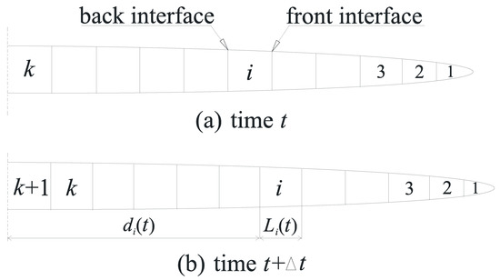
Figure 1.
Schematic diagram of the fracture propagation model.
The width equation uses the PKN analytical solution for double wing fractures with fluid loss [44]:
where:
where is the rock Poisson’s ratio, E is the rock elastic modulus (Pa), is the fracture height (m), C is the fluid loss coefficient (m/s1/2), is the apparent viscosity of the power law fluid (Pa·s), K is the fluid consistency coefficient (Pa·sn), n is the flow index, Q is the injection rate (m3/s), and is the average width along the fracture height (m). For the PKN model, .
Because the fracture length solution of the PKN model does not satisfy the flow continuity equation, the following continuity equation is used for fracture half-length calculation (where spurt loss is ignored):
where:
The volume of the fluid loss for each element is limited as follows:
Because the fracture half-length cannot be solved explicitly, an iterative method is used. First, an initial fracture half-length is assumed, and then the fracture width distribution is solved by Equation (8). We can substitute it into Equation (10) to check whether the continuity equation is satisfied. If it is not, then we assume another fracture half-length and calculate again. In general, the fracture half-length increases with time. So, the assumed value can be set as the previous value plus a small increment until it finally satisfies the continuity equation. When both the fracture width and half-length have been determined, the fluid element space in the fracture should be reassigned. The remaining volume of each fluid element after pumping for time segments is:
According to the remaining volume of each fluid element, starting from the fracture tip, we calculate in turn the distance of the back interface of element to the fracture entry:
As the model satisfies the continuity equation, then the following condition will be satisfied naturally:
Thus, the length of each fluid element becomes:
The proppant concentration in the fluid element can be calculated as:
Because fluid loss occurs during fracturing, sand-laden fluid that was injected early is subject to a long loss time; hence, the sand ratio of the injected fluid at early times should be relatively small. As the loss time of sand-laden fluid injected at a later stage is short, the sand ratio of the injected fluid can be relatively large. Thus, at the end of injection, the proppant in the whole fracture will be evenly distributed. For the convenience of operation, the staged proppant pumping schedule is usually used. It means that one constant sand ratio is maintained over a period of time. When the injection of these portions of sand-laden fluid is finished, the sand ratio is then changed. In this paper, the sand ratio is increased according to the following power function to ensure that the proppant is distributed as evenly as possible, so as to reach the desired proppant concentration:
where is the sand ratio (representing the ratio of proppant to fluid volume), and are coefficients (in this paper, is referred to as the proppant pumping curve index), and is the proppant pumping sequence. If all the proppants are to be injected through 10 times, then the value of is an integer from 1–10. In this paper, the proppant pumping times and the maximum sand ratio will be determined empirically. Then, for a given value of coefficient , the corresponding coefficient can be determined. Thus, the optimization of the complicated proppant pumping schedule can be simplified as the optimization of the single coefficient .
After the injection has finished, the pad fluid continues to be lost and the front of the fracture will close. Thus, the half-length of the propped fracture can be set as the length in which proppant is present. If the proppant concentration in the direction of the fracture width has not reached a certain value, then the fracture will close and the fracture width will decrease until the proppant concentration reaches the desired value. The final width is the propped fracture width. The average fracture width is used in the UFD method regardless of the fracture shape. Figure 2a shows the state of the fracture immediately after the end of injection. Figure 2b shows the state of the propped fracture.
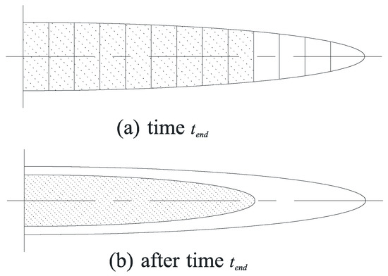
Figure 2.
Schematic diagram of fracture closure.
This simulation needs to find the optimal treatment parameters in order to satisfy both the fracture half-length and width. So, the objective of the treatment optimization is to minimize the following error function:
where is the calculated fracture half-length (m), is the optimal fracture half-length (m), is the calculated fracture width (m), and is the optimal fracture width (m).
The basic flowchart of the proposed fracturing treatment optimization method based on the UFD is shown in Figure 3.
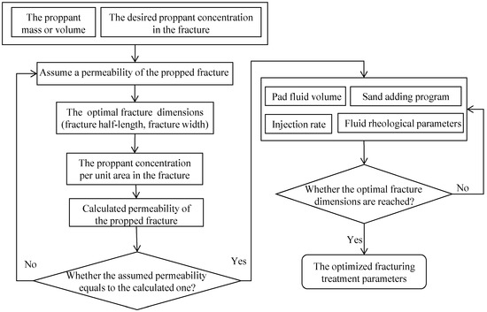
Figure 3.
Flowchart of the proposed optimization method.
3. Results and Discussion
3.1. Basic Parameters
To validate the proposed method, it was applied to a case study reservoir: that of the Daniudi Gas Field located at the junction of the city of Yulin, Shaanxi Province and the city of Ordos, Inner Mongolia Autonomous Region, China. It contains lower Paleozoic marine carbonate rock as one of the main gas-bearing strata. Its basic parameters are listed in Table 1. The homogeneous rock is presented in this case study for illustration. Nevertheless, the heterogeneous rocks are usually divided into several homogeneous segments [19] and the proposed method can also be used for each segment respectively.

Table 1.
Reservoir properties and fixed fracturing parameters.
3.2. Optimization Method and Results
A proppant volume of 18 m3 is used to illustrate the optimization process and results. First of all, the desired proppant concentration is set to 1000 kg/m3, which is related to the proppant pumping schedule and will be discussed later in the paper. According to the actual situation in the field, the maximum sand ratio is set to 35% and the proppant pumping schedule is divided into eight stages. The maximum proppant concentration during fracture propagation is 700 kg/m3. The other treatment parameters will be optimized to satisfy the desired proppant concentration, optimal propped fracture conductivity and dimensions.
As a matter of fact, all the related treatment parameters can be optimized automatically by an exhausted search method. However, due to the field treatment capability, if certain constraints are set to some parameters [52], then the optimization efficiency can be increased significantly. Next methods demonstrate how the treatment parameter constraints facilitate the optimization procedure and how they affect the optimization result.
Usually, the pad fluid volume is one of the key parameters to be optimized. If the injection rate, fluid rheological parameters and proppant pumping schedule can be selected according to the actual treatment conditions, and then the pad fluid volume needs to be optimized automatically. Taking an injection rate Q of 5 m3/min as an example, if the fluid’s apparent viscosity is set as 58 mPa·s (for instance, the fluid consistency coefficient K is set to 0.7 Pa·sn, and the flow index n is set to 0.6), and the proppant pumping curve index b is set as 0.63, then the curve for the calculated propped fracture half-length and width versus different pad fluid volumes can be illustrated, as in Figure 4 and Figure 5. For the sake of comparison, the optimal fracture half-length and width are also plotted in the figure as horizontal lines. As shown in the figures, the propped fracture half-length decreases while the propped fracture width increases with increasing pad fluid volume. When the calculated fracture half-length curve intersects the optimal fracture half-length horizontal line and the calculated fracture width curve intersects the optimal fracture width horizontal line, the optimal pad fluid volume can be obtained.
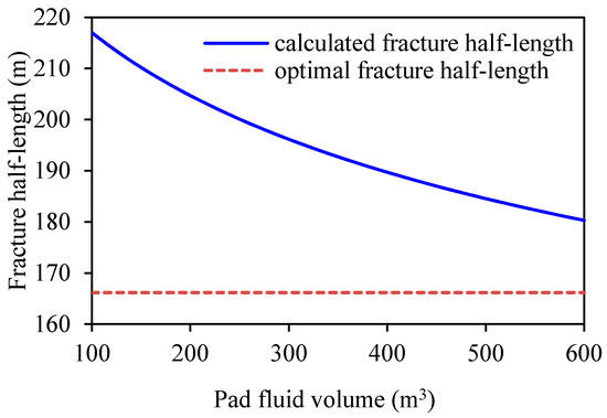
Figure 4.
Curves of propped fracture half-length vs. pad fluid volume for the original design.
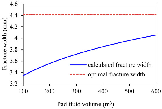
Figure 5.
Curves of propped fracture width vs. pad fluid volume for the original design.
As shown from the figures, within a certain range of pad fluid volumes, no optimization result can be acquired. Nevertheless, the design scheme can be adjusted in two ways. The first is to increase the injection rate and the second is to increase the fluid’s apparent viscosity. For the first adjusted scheme, if the injection rate is increased to 7 m3/min, then new curves are obtained, as illustrated in Figure 6 and Figure 7. As shown from these figures, an optimal pad fluid volume within the given range can be acquired.
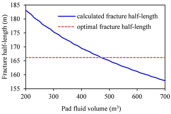
Figure 6.
Curves of propped fracture half-length vs. pad fluid volume for the first adjusted design.
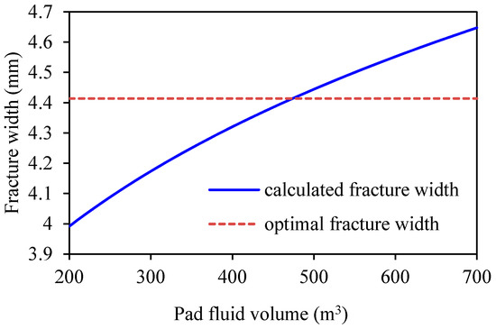
Figure 7.
Curves of propped fracture width vs. pad fluid volume for the first adjusted design.
For the second adjusted scheme, if the fluid’s apparent viscosity is increased to 201 mPa·s (for instance, the fluid consistency coefficient K is set to 0.7 Pa·sn, and the flow index n is set to 0.8), then new curves are as illustrated in Figure 8 and Figure 9. As shown from these figures, the optimal pad fluid volume within the given range can be acquired.
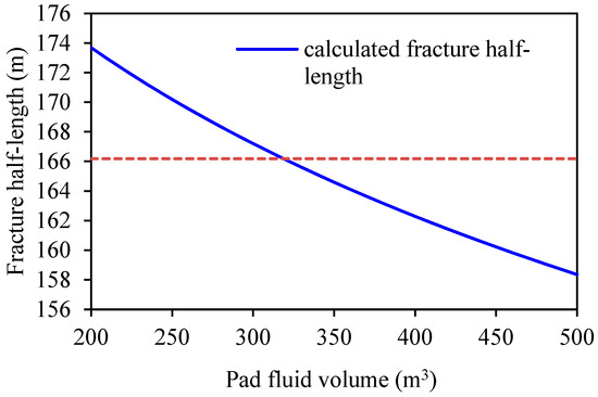
Figure 8.
Curves of propped fracture half-length vs. pad fluid volume for the second adjusted design.
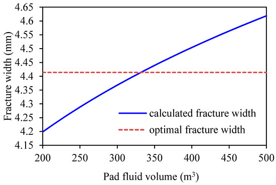
Figure 9.
Curves of propped fracture width vs. pad fluid volume for the second adjusted design.
According to the above analysis, the treatment parameters that satisfy the optimal fracture dimensions are not unique. For the above two adjusted designs, if the field equipment can meet the required injection rate, then the first adjusted design will be the better option.
As a matter of fact, more parameters can be optimized. This paper proposes the interval search method for automatic optimization. If we set the injection rate as 7 m3/min, the range of other parameters needing to be optimized and the search step lengths are as listed in Table 2. The search range can be tuned according to the actual treatment conditions and the search step length can also be tuned based on the optimization accuracy and the calculation efficiency. Generally, a coarse-to-fine search strategy is used. During this optimization, the search step length for pad fluid volume is initially set to 50, and then tuned to 10 to obtain a more accurate result. The complete optimization results are listed in Table 3.
Table 2.
Ranges of parameters used in optimization.
Table 3.
Optimization results.
3.3. General Discussion
For rapid optimization, the injection rate and fluid rheological parameters are preset or tuned within certain ranges according to the actual treatment conditions, and the pad fluid volume needs to be optimized automatically. To this end, it is important to analyze the influences of the injection rate and fluid rheological parameters on the optimization results. Furthermore, the reservoir permeability has a strong influence on the optimization results, which will be also discussed in this section. Although the discussions used the specific data above, they are quite general and very useful for the field optimization design especially using the proposed methods in this paper. Moreover, the findings in this section are consistent well with the established knowledge. They are presented here for completeness.
3.3.1. Injection Rate
Based on the above data, we consider several injection rates: 4, 5, 6, 7, 8 and 9 m3/min. Other parameters, including proppant pumping curve index b and fluid rheological parameters are obtained from Table 3 and held constant. Then, the curve describing the relationship between pad fluid volume and injection rate is obtained, as shown in Figure 10. To generate the same fracture with the same fluid and proppant pumping schedule, the required pad fluid volume decreases with increasing injection rate. Note that when the injection rate is small, the required pad fluid volume is excessively large, which is unfeasible in terms of treatment difficulty and cost. Therefore, it is suggested to select a larger injection rate, within the treatment limitations, in order to reduce the amount of pad fluid used.
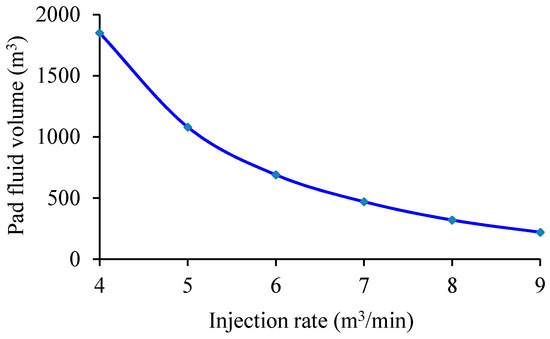
Figure 10.
Curve describing the relationship between pad fluid volume and injection rate.
3.3.2. Fluid’s Apparent Viscosity
Based on the above data, we can take different fluid’s apparent viscosities, such as 20 mPa·s (for instance, if K = 0.46 Pa·sn and n = 0.5), 30 mPa·s (K = 0.5 Pa·sn and n = 0.55), 58 mPa·s (K = 0.7 Pa·sn and n = 0.6), 80 mPa·s (K = 0.71 Pa·sn and n = 0.65), and 100 mPa·s (K = 0.79 Pa·sn and n = 0.67). Other parameters come from Table 3 and are held constant. Then, the curve describing the relationship between the pad fluid volume and the fluid’s apparent viscosity is as shown in Figure 11. To generate the same fracture with the same injection rate and proppant pumping schedule, the required pad fluid volume decreases with increasing apparent viscosity of the fluid. Note that when the fluid’s apparent viscosity is small, the required pad fluid volume is excessively large, which is unfeasible in terms of treatment difficulty and cost. Therefore, it is concluded that a larger apparent fluid viscosity reduces the amount of pad fluid used.
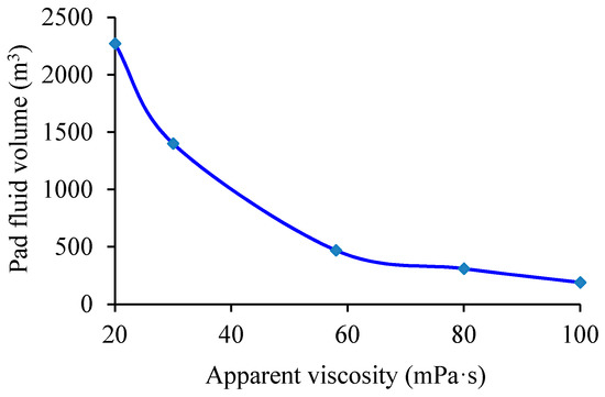
Figure 11.
Curve of the relationship between pad fluid volume and its apparent viscosity.
3.3.3. Reservoir Permeability
Based on the above data, we now consider reservoir permeability values of: 0.001, 0.01, 0.1, 0.2, 0.35, 0.46 and 1 md. Figure 12 shows the optimal propped fracture half-lengths and widths for various reservoir permeabilities. With increases in reservoir permeability, the optimal fracture half-length decreases while the optimal fracture width increases. This is consistent with established knowledge. That is to say, for very low permeability reservoirs, long and narrow fractures should be created. For low-to-medium permeability reservoirs, short and wide fractures should be created. Figure 13 shows the optimal dimensionless fracture conductivity and the maximum dimensionless productivity index for different reservoir permeabilities. From the figure, we can see that with decreases in reservoir permeability, the maximum dimensionless productivity increases. Despite this, as actual production is proportional to reservoir permeability, for very low-permeability reservoirs, absolute production remains low.
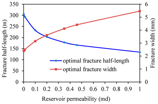
Figure 12.
Optimal propped fracture half-lengths and widths vs. reservoir permeability.
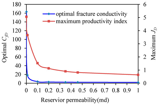
Figure 13.
Optimal and maximum values vs. reservoir permeability.
During the optimization for various reservoir permeabilities, other parameters, including the injected proppant volume on the ground, injection rate, and desired proppant concentration are taken from Table 3 and kept invariable. The pad fluid volume and the fluid rheological parameters are optimized automatically. Figure 14 shows the optimized pad fluid volume and the fluid’s apparent viscosity for different reservoir permeabilities. The figure shows that with increases in reservoir permeability, the pad fluid volume increases and the fluid’s apparent viscosity increases accordingly. Thus, it can be seen that for very low permeability reservoirs, low viscosity fluid should be used, and for low-to-medium permeability reservoirs, high viscosity fluid should be used. This is also consistent with established knowledge.
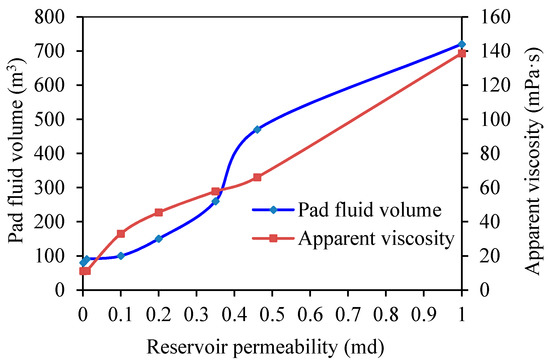
Figure 14.
Optimized pad fluid volume and fluid’s apparent viscosity vs. reservoir permeability.
3.4. Special Discussion
Besides the general parameters discussed above, two other important parameters are introduced in this paper for coupling the fracturing treatment optimization and fracture geometry optimization: desired proppant concentration in the fracture and injected proppant volume on the ground. The desired proppant concentration in the fracture is used to solve the optimal fracture half-length and width. It also affects the treatment parameters in the fracture propagation model to reach the optimal fracture dimensions. The determination of it will be discussed in this section.
The injected proppant volume on the ground is also a key factor for fracturing. It determines the optimal fracture dimensions. Generally, there are two methods for optimizing it. The first is to select the maximum proppant volume that can be injected by the field treatment equipment, under the condition that all the treatment parameters are optimized to obtain the maximum productivity index using the proposed method. The second is to determine the injected proppant volume so as to maximize the NPV. For illustration, the influence of the injected proppant volume on the treatment parameter optimization results will be discussed, and the injected proppant volume used for the treatment will be determined using the first method.
3.4.1. Desired Proppant Concentration in the Fracture
When the desired proppant concentration is preset, it can be reached through optimization of the treatment parameters. Once both the desired proppant concentration and the optimal fracture half-length are satisfied during the optimization process, the fracture width will be satisfied naturally. Usually, the desired proppant concentration can be obtained through the parameter optimization of the proppant pumping curve index b. Based on the above data, we consider several proppant concentrations in the fracture: 800, 900, 1000, 1100 and 1200 kg/m3. Other parameters, including the injected proppant volume on the ground, the injection rate, and fluid rheological parameters, are taken from Table 3 and held constant.
Figure 15 shows the optimal propped fracture half-lengths and widths with different proppant concentrations. Figure 16 shows the optimal dimensionless fracture conductivity and the maximum dimensionless productivity index with different proppant concentrations. As shown by the figures, with increasing desired proppant concentration, both the optimal fracture half-length and width decrease, as does the maximum dimensionless productivity index.
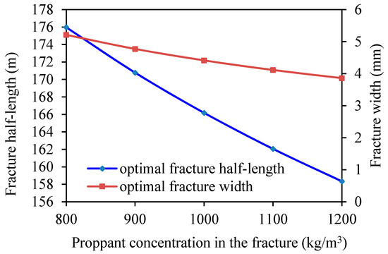
Figure 15.
Optimal propped fracture half-lengths and widths according to proppant concentration.
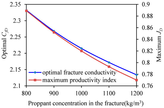
Figure 16.
Optimal values of and maximum according to proppant concentration
Figure 17 shows optimized proppant pumping curves for various desired proppant concentrations. However, a stepped proppant pumping schedule, rather than a continuous one, is used in actual fracturing treatments. This is represented by the dashed line in Figure 17. The optimized proppant pumping curve coefficients a, indexes b, and actual proppant pumping schedules for various desired proppant concentrations are listed in Table 4. As shown in the table, with increases of the desired proppant concentration, the initial sand ratio (the 1st stage sand ratio) increases and the differences between the sand ratios of subsequent stages decrease. This style is rather disadvantageous for use in actual treatments, because the sand-laden fluid with the initial sand ratio stays in the fracture for a relatively long time, and the proppant concentration will continuously increase due to fluid loss. In this situation, a sand plug is likely to occur. In addition, as shown in Figure 16, with increasing desired proppant concentration, the maximum dimensionless productivity index decreases. Therefore, a high desired proppant concentration is not advantageous.
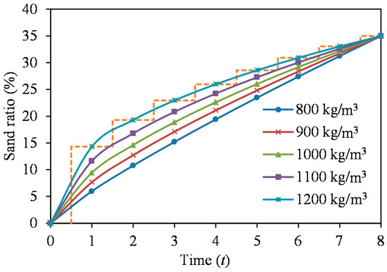
Figure 17.
Optimized proppant pumping curves for various desired proppant concentrations.
Table 4.
Stepped proppant pumping schedule for various desired proppant concentrations.
With the decreases in the desired proppant concentration, the initial sand ratio decreases and the differences between the sand ratios of subsequent stages increase. This style is advantageous for avoiding sand plugs. However, from Figure 18 note that the optimal pad fluid volume increases with decreasing desired proppant concentration. In particular, when the desired proppant concentration is relatively small, the pad fluid volume becomes very large, which is unfeasible in terms of treatment difficulty and cost. Based on the above analysis, there is a reasonable range for the desired proppant concentration in the fracture. In this paper, the desired proppant concentration is set to 1000 kg/m3, which provides a reference for actual designs.
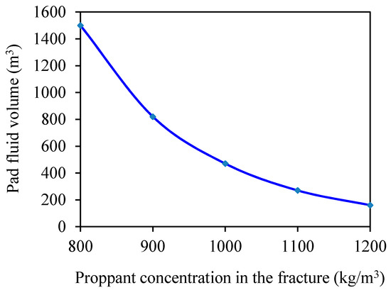
Figure 18.
Optimal pad fluid volume vs. desired proppant concentration.
3.4.2. Injected Proppant Volume on the Ground
Based on the above data, we now consider several injected proppant volumes: 6, 12, 18, 24 and 30 m3. Figure 19 shows the optimal fracture half-lengths and widths for different injected proppant volumes. Figure 20 shows the optimal dimensionless fracture conductivity and the maximum dimensionless productivity index for different injected proppant volumes. The figures show that with increases of injected proppant volume, both the optimal fracture half-length and width increase, and the maximum dimensionless productivity index increases as well.
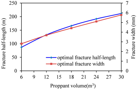
Figure 19.
Optimal fracture half-lengths and widths vs. injected proppant volume.
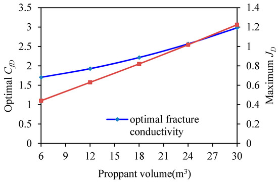
Figure 20.
Optimal and maximum values vs. injected proppant volume.
However, with increases in the injected proppant volume, the treatment cost and difficulty will both increase. For different injected proppant volumes, other parameters, including the desired proppant concentration, are taken from Table 3 and held constant. The pad fluid volume, fluid rheological parameters and injection rate are to be optimized next. Figure 21 and Figure 22 show the optimized pad fluid volume, fluid apparent viscosity, and injection rate for different injected proppant volumes. From the figures, with increases of injected proppant volume, the pad fluid volume increases, the fluid apparent viscosity increases and the injection rate also increases. Thus, in spite of the increase in the dimensionless productivity index resulting from the increase in proppant volume, the treatment becomes more and more difficult. Therefore, the injected proppant volume should be controlled within a suitable range according to the treatment conditions in order to use it efficiently.
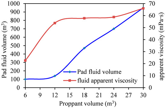
Figure 21.
Optimized pad fluid volume and fluid’s apparent viscosity vs. injected proppant volume.
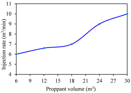
Figure 22.
Optimized injection rate vs. injected proppant volume.
4. Conclusions
This paper presented a method to couple the fracturing treatment optimization and fracture geometry optimization in order to maximize the dimensionless productivity index. By introducing a desired proppant concentration in the fracture, the optimal fracture half-length and width can be solved based on UFD method and an iterative approach. Moreover, a rapid semi-analytical fracture propagation model was proposed in combination with an interval search method to optimize fracturing treatment parameters in order to reach the optimal fracture dimensions. Based on the case study and analyses contained in this paper, the following conclusions can be drawn:
- (1)
- Through the semi-analytical fracture propagation model and the treatment optimization method, the desired proppant concentration in the fracture can be achieved by optimizing the proppant pumping curve index b. The optimal fracture half-length can be achieved by optimizing parameters such as pad fluid volume, injection rate, and fluid rheological parameters. Once both the desired proppant concentration and optimal fracture half-length are achieved, the optimal fracture width is also achieved naturally.
- (2)
- In order to obtain the optimal fracture dimensions, the treatment parameters are not unique. The optimal treatment parameters can be determined according to both the actual treatment conditions in the field and the optimization procedure. The prior empirical knowledge about the actual fracturing treatment can also make the optimization more efficiently.
- (3)
- For the sake of rapid calculation, a 2D fracture propagation model was used. This optimization method can provide complete and reasonable fracturing treatment parameters that meet the basic requirements of field designs and provide a reference for finer fracturing simulations and designs if necessary.
Author Contributions
Conceptualization, K.A. and H.G.; Methodology, K.A.; Software, H.G.; Validation, G.J.; Investigation, K.A. and G.J.; Data Curation, G.J.; Writing-Original Draft Preparation, K.A.; Writing-Review & Editing, H.G.; Visualization, H.G.; Supervision, L.D.; Project Administration, L.D.; Funding Acquisition, K.A.
Acknowledgments
This research was supported by the China National High Technology Research and Development Program 863 (Grant No. 2013AA064503), the National Natural Science Foundation of China (41672364, 41602373).
Conflicts of Interest
The authors declare no conflict of interest.
Appendix A. Unified Fracture Design (UFD) Method
We first define the penetration ratio:
and dimensionless fracture conductivity:
where is the fracture half-length (m); is the length of the drainage area (m); is the permeability of the propped fracture (md); is the permeability of the reservoir (md); and is the average width of the propped fracture (m).
If the volume of the propped fracture is constant, then the proppant number is also constant:
Define:
where is the width of the drainage area (m); is the volume of the propped fracture (m3); is the volume of the drainage area (m3); and is the thickness of the reservoir (m).
Through numerical calculations, Valkό and Economides [54,57] found that the maximum dimensionless productivity index and the corresponding optimal dimensionless fracture conductivity can be uniquely determined given the proppant number. That is, the maximum dimensionless productivity index and optimal dimensionless fracture conductivity are functions of the proppant number.
Introduce the shape factor CA and the equivalent proppant number Nprop,e. Values of CA are shown in Table A1.
Table A1.
Dietz shape factors for a range of aspect ratios.
Table A1.
Dietz shape factors for a range of aspect ratios.
| 0.1 | 0.2 | 0.25 | 0.3 | 0.4 | 0.5 | 0.6 | 0.7 | 0.8 | 0.9 | 1.0 | |
|---|---|---|---|---|---|---|---|---|---|---|---|
| 0.025 | 2.36 | 5.38 | 9.00 | 16.17 | 21.84 | 25.80 | 28.36 | 29.89 | 30.66 | 30.88 |
Using the shape factor, the equivalent proppant number can be written as:
The maximum dimensionless productivity index and the optimal dimensionless fracture conductivity in rectangular reservoirs can be described by the following equations.
- (1)
- When : align
- (2)
- When :
where:
The related constants are from Table A2.
Table A2.
Constants in F-function.
Table A2.
Constants in F-function.
| 1 | 0.7 | 0.5 | 0.25 | 0.2 | 0.1 | |
| a | 17.2 | 17.4 | 21.4 | 38.3 | 35 | 30.6 |
| b | 54.5 | 55.5 | 54.3 | 46 | 59 | 89.6 |
| c | 52.5 | 53.3 | 56.3 | 71.1 | 70 | 70.2 |
| d | 16.9 | 16.9 | 16.9 | 15.84 | 16.3 | 17.8 |
| a’ | 10 | |||||
| b’ | 36 | |||||
| c’ | 33 | |||||
References
- Hareland, G.; Rampersad, P.; Dharaphop, J.; Sasnanand, S. Hydraulic Fracturing Design Optimization. In Proceedings of the 1993 Eastern Regional Conference & Exhibition, Pittsburgh, PA, USA, 2–4 November 1993. [Google Scholar]
- Lynk, J.M.; Papandrea, R.; Collamore, A.; Quinn, T.; Cazeneuve, E.; Centurion, S. Hydraulic fracture completion optimization in Fayetteville shale: Case study. Int. J. Geomech. 2016, 17, 04016053. [Google Scholar] [CrossRef]
- Roussel, N.P.; Sharma, M.M. Optimizing Fracture Spacing and Sequencing in Horizontal-Well Fracturing. In Proceedings of the 2010 SPE International Symposium and Exhibition on Formation Damage Control, Lafayette, LA, USA, 10–12 February 2010. [Google Scholar]
- Jamiolahmady, M.; Sohrabi, M.; Mahdiyar, H. Optimization of Hydraulic Fracture Geometry. In Proceedings of the 2009 SPE Offshore Europe Oil & Gas Conference & Exhibition, Aberdeen, UK, 8–11 September 2009. [Google Scholar]
- Manrique, J.F.; Poe, B.D. Evaluation and Optimization of Low Conductivity Fractures. In Proceedings of the SPE Hydraulic Fracturing Technology Conference, College Station, TX, USA, 29–31 January 2007. [Google Scholar]
- Bruce, R.M.; Lucas, W.B.; Henry, R.J.; Michael, G.L. Optimization of Multiple Transverse Hydraulic Fractures in Horizontal Wellbores. In Proceedings of the SPE Unconventional Gas Conference, Pittsburgh, PA, USA, 23–25 February 2010. [Google Scholar]
- Zeng, F.; Zhao, G. The optimal hydraulic fracture geometry under non-Darcy flow effects. J. Petrol. Sci. Eng. 2010, 72, 143–157. [Google Scholar] [CrossRef]
- Siddhamshetty, P.; Yang, S.; Kwon, S.I. Modeling of hydraulic fracturing and designing of online pumping schedules to achieve uniform proppant concentration in conventional oil reservoirs. Comput. Chem. Eng. 2018, 114, 306–317. [Google Scholar] [CrossRef]
- Yang, S.; Siddhamshetty, P.; Kwon, S.I. Optimal pumping schedule design to achieve a uniform proppant concentration level in hydraulic fracturing. Comput. Chem. Eng. 2017, 101, 138–147. [Google Scholar] [CrossRef]
- Rahman, M.M.; Rahman, M.K.; Rahman, S.S. Optimizing treatment parameters for enhanced hydrocarbon production by hydraulic fracturing. J. Can. Pet. Technol. 2003, 42, 38–46. [Google Scholar] [CrossRef]
- Poulsen, D.K.; Soliman, M.Y. A Procedure for Optimal Hydraulic Fracturing Treatment Design. In Proceedings of the SPE Eastern Regional Meeting, Columbus, OH, USA, 12–14 November 1986. [Google Scholar]
- Soliman, M.Y.; Pongratz, R.; Rylance, M.; Prather, D. Fracture Treatment Optimization for Horizontal Well Completion. In Proceedings of the 2006 SPE Russian Oil and Gas Technical Conference and Exhibition, Moscow, Russia, 3–6 October 2006. [Google Scholar]
- Lopez-Hernandez, H.; Valkó, P.P.; Tai, T.P. Optimum Fracture Treatment Design Minimizes the Impact of Non-Darcy Flow Effects. In Proceedings of the SPE Annual Technical Conference and Exhibition, Houston, TX, USA, 26–29 September 2004. [Google Scholar]
- Kong, B.; Fathi, E.; Ameri, S. Coupled 3-D numerical simulation of proppant distribution and hydraulic fracturing performance optimization in Marcellus shale reservoirs. Int. J. Coal Geol. 2015, 147–148, 35–45. [Google Scholar] [CrossRef]
- Mahdiyar, H.; Jamiolahmady, M. Optimization of hydraulic fracture geometry in gas condensate reservoirs. Fuel 2014, 119, 27–37. [Google Scholar] [CrossRef]
- Wang, X.; Wang, Z.; Zeng, Q.; Yang, G.; Chen, T.; Guo, X. Non-Darcy effect on fracture parameters optimization in fractured CBM horizontal well. J. Nat. Gas Sci. Eng. 2015, 27, 1438–1445. [Google Scholar] [CrossRef]
- Masoomi, R.; Viktorovich, D.S. Simulation and optimization of the hydraulic fracturing operation in a heavy oil reservoir in southern Iran. J. Eng. Sci. Technol. 2017, 12, 241–255. [Google Scholar]
- Wang, J.; Jia, A. A general productivity model for optimization of multiple fractures with heterogeneous properties. J. Nat. Gas Sci. Eng. 2014, 21, 608–624. [Google Scholar] [CrossRef]
- Zeng, F.H.; Ke, Y.B.; Guo, J.C. An optimal fracture geometry design method of fractured horizontal wells in heterogeneous tight gas reservoirs. Sci. China Technol. Sci. 2016, 59, 241–251. [Google Scholar] [CrossRef]
- Atefeh, J.; Behnam, J. Optimization of hydraulic fracturing design under spatially variable shale fracability. J. Pet. Sci. Eng. 2016, 138, 174–188. [Google Scholar]
- Zhang, Z.; Li, X.; Yuan, W.; He, J.; Li, G.; Wu, Y. Numerical analysis on the optimization of hydraulic fracture networks. Energies 2015, 8, 12061–12079. [Google Scholar] [CrossRef]
- Zeng, F.H.; Guo, J.C. Optimized design and use of induced complex fractures in horizontal wellbores of tight gas reservoirs. Rock Mech. Rock Eng. 2016, 49, 1411–1423. [Google Scholar] [CrossRef]
- Chen, M.; Sun, Y.; Fu, P.; Charles, R.; Lu, Z.; Charles, H.T.; Thomas, A.B. Surrogate-based optimization of hydraulic fracturing in pre-existing fracture networks. Comput. Geosci. 2013, 58, 69–79. [Google Scholar] [CrossRef]
- Balen, R.M.; Mens, H.Z.; Economides, M.J. Applications of the Net Present Value (NPV) in the Optimization of Hydraulic Fractures. In Proceedings of the SPE Eastern Regional Meeting, Charleston, WV, USA, 1–4 November 1988. [Google Scholar]
- Kim, H.; Querin, O.M.; Steven, G.P. On the development of structural optimization and its relevance in engineering design. Des. Stud. 2002, 23, 85–102. [Google Scholar] [CrossRef]
- Hariharan, K.; Balaji, C. Material optimization: A case study using sheet metal-forming analysis. J. Mater. Process. Technol. 2009, 209, 324–331. [Google Scholar] [CrossRef]
- Chisari, C.; Bedon, C. Multi-objective optimization of FRP jackets for improving the seismic response of reinforced concrete frames. Am. J. Eng. Appl. Sci. 2016, 9, 669–679. [Google Scholar] [CrossRef]
- Rahman, M.M.; Rahman, M.K.; Rahman, S.S. An integrated model for multi-objective design optimization of hydraulic fracturing. J. Pet. Sci. Eng. 2001, 31, 41–62. [Google Scholar] [CrossRef]
- Yang, C.; Vyas, A.; Datta-Gupta, A.; Ley, S.B.; Biswas, P. Rapid multistage hydraulic fracture design and optimization in unconventional reservoirs using a novel Fast Marching Method. J. Pet. Sci. Eng. 2017, 156, 91–101. [Google Scholar] [CrossRef]
- Lee, S.; Min, B.; Wheeler, M.F. Optimal design of hydraulic fracturing in porous media using the phase field fracture model coupled with genetic algorithm. Comput. Geosci. 2018, 3, 833–849. [Google Scholar] [CrossRef]
- Mohaghegh, S.; Balanb, B.; Platon, V.; Ameri, S. Hydraulic fracture design and optimization of gas storage wells. J. Pet. Sci. Eng. 1999, 23, 161–171. [Google Scholar] [CrossRef]
- Shahab, M.; Andrei, P.; Sam, A. Intelligent Systems Can Design Optimum Fracturing Jobs. In Proceedings of the 1999 SPE Eastern Regional Conference and Exhibition, Charleston, WV, USA, 21–22 October 1999. [Google Scholar]
- Gorucu, S.E.; Ertekin, T. Optimization of the Design of Transverse Hydraulic Fractures in Horizontal Wells Placed in Dual Porosity Tight Gas Reservoirs. In Proceedings of the SPE Middle East Unconventional Gas Conference and Exhibition, Muscat, Oman, 31 January–2 February 2011. [Google Scholar]
- Rueda, J.I. Using a Mixed Integer Linear Programming Technique to Optimize a Fracture Treatment Design. In Proceedings of the 1994 SPE Eastern Regional Conference and Exhibition, Charleston, WV, USA, 8–10 November 1994. [Google Scholar]
- Li, J.C.; Gong, B.; Wang, H.G. Mixed integer simulation optimization for optimal hydraulic fracturing and production of shale gas fields. Eng. Optim. 2015, 48, 1378–1400. [Google Scholar] [CrossRef]
- Queipo, N.V.; Verde, A.J.; Canelón, J.; Pintos, S. Efficient global optimization for hydraulic fracturing treatment design. J. Pet. Sci. Eng. 2002, 35, 151–166. [Google Scholar] [CrossRef]
- Wangen, M. Finite element modeling of hydraulic fracturing in 3D. Comput. Geosci. 2013, 17, 647–659. [Google Scholar] [CrossRef]
- Gordeliy, E.; Peirce, A. Implicit level set schemes for modeling hydraulic fractures using the XFEM. Comput. Methods Appl. Mech. Eng. 2013, 266, 125–143. [Google Scholar] [CrossRef]
- Li, L.; Xia, Y.; Huang, B.; Zhang, L.; Li, M.; Li, A. The behaviour of fracture growth in Sedimentary rocks: A numerical study based on hydraulic fracturing processes. Energies 2016, 9, 169. [Google Scholar] [CrossRef]
- Wang, J.; Li, H.; Wang, Y.; Li, Y.; Jiang, B.; Luo, W. A new model to predict productivity of multiple-fractured horizontal well in naturally fractured reservoirs. Math. Probl. Eng. 2015, 2015, 892594. [Google Scholar] [CrossRef]
- Liu, Q.; Chen, Y.; Wang, W.; Liu, H.; Hu, X.; Xie, Y. A productivity prediction model for multiple fractured horizontal wells in shale gas reservoirs. J. Nat. Gas Sci. Eng. 2017, 42, 252–261. [Google Scholar] [CrossRef]
- Medeiros, F.; Ozkan, E.; Kazemi, H. Productivity and Drainage Area of Fractured Horizontal Wells in Tight Gas Reservoirs. In Proceedings of the 2007 SPE Rocky Mountain Oil & Gas Technology Symposium, Denver, CO, USA, 16–18 April 2007. [Google Scholar]
- Luo, W.; Wang, X.; Feng, Y.; Tang, C.; Zhou, Y. Productivity analysis for a vertically fractured well under non-Darcy flow condition. J. Pet. Sci. Eng. 2016, 146, 714–725. [Google Scholar] [CrossRef]
- Nordgren, R.P. Propagation of a vertical hydraulic fracture. Soc. Pet. Eng. J. 1972, 12, 306–314. [Google Scholar] [CrossRef]
- Valkó, P.P.; Economides, M.J. Hydraulic Fracture Mechanics; John Wiley & Sons: New York, NY, USA, 1995. [Google Scholar]
- Kovalyshen, Y.; Detournay, E. A reexamination of the classical PKN model of hydraulic fracture. Transp. Porous Media 2010, 81, 317–339. [Google Scholar] [CrossRef]
- Palmer, I.D.; Carroll, H.B. Numerical Solution for Height and Elongated Hydraulic Fractures. In Proceedings of the 1983 SPE/DOE Symposium on Low Permeability, Denver, CO, USA, 14–16 March 1983. [Google Scholar]
- Rahman, M.M.; Rahman, M.K. A Review of Hydraulic Fracture Models and Development of an Improved Pseudo-3D Model for Stimulating Tight Oil/Gas Sand. Energy Sources 2010, 32, 1416–1436. [Google Scholar] [CrossRef]
- Pitakbunkate, T.; Yang, M.; Valkó, P.P.; Economides, M.J. Hydraulic Fracture Optimization with a P-3D Model. In Proceedings of the SPE Production and Operations Symposium, Oklahoma City, OK, USA, 27–29 March 2011. [Google Scholar]
- Economides, M.J.; Demarchos, A.S. Benefits of a p-3D over a 2D Model for Unified Fracture Design. In Proceedings of the 2008 SPE International Symposium and Exhibition on Formation Damage Control, Lafayette, LA, USA, 13–15 February 2008. [Google Scholar]
- Meng, H.Z.; Brown, K.E. Coupling of Production Forecasting, Fracture Geometry Requirements and Treatment Scheduling in the Optimum Hydraulic Fracture Design. In Proceedings of the SPE/DOE Low Permeability Reservoirs Symposium, Denver, CO, USA, 18–19 May 1987. [Google Scholar]
- Rahman, M.M. Constrained hydraulic fracture optimization improves recovery from low permeable oil reservoirs. Energy Sources Part A 2008, 30, 536–551. [Google Scholar] [CrossRef]
- Valkó, P.P.; Economides, M.J. Heavy Crude Production from Shallow Formations: Long Horizontal Wells Versus Horizontal Fractures. In Proceedings of the SPE International Conference on Horizontal Well Technology, Calgary, AB, Canada, 1–4 November 1998. [Google Scholar]
- Economides, M.J.; Oligeny, R.E.; Valkó, P.P. Unified Fracture Design; Orsa Press: Houston, TX, USA, 2002. [Google Scholar]
- Demarchos, A.S.; Chomatas, A.S.; Economides, M.J. Pushing the Limits in Hydraulic Fracture Design. In Proceedings of the SPE International Symposium and Exhibition on Formation Damage Control, Lafayette, LA, USA, 18–20 February 2004. [Google Scholar]
- Romero, D.J.; Valkó, P.P.; Economides, M.J. Optimization of the Productivity Index and the Fracture Geometry of a Stimulated Well with Fracture Face and Choke Skins. In Proceedings of the 2002 SPE International Symposium and Exhibition on Formation Damage Control, Lafayette, LA, USA, 20–21 February 2003. [Google Scholar]
- Daal, J.A.; Economides, M.J. Optimization of Hydraulically Fractured Wells in Irregularly Shaped Drainage Areas. In Proceedings of the 2006 SPE International Symposium and Exhibition on Formation Damage Control, Lafayette, LA, USA, 15–17 February 2006. [Google Scholar]
- Martin, A.N.; Economides, M.J. Best Practices for Candidate Selection, Design and Evaluation of Hydraulic Fracture Treatments. In Proceedings of the SPE Production and Operations Conference and Exhibition, Tunis, Tunisia, 8–10 June 2010. [Google Scholar]
- Bhattacharya, S.; Nikolaou, M.; Economides, M.J. Unified Fracture Design for very low permeability reservoirs. J. Nat. Gas Sci. Eng. 2012, 9, 184–195. [Google Scholar] [CrossRef]
- Mukherjee, H.; Economides, M.J. A parametric comparison of horizontal and vertical well performance. SPE Form. Eval. 1991, 6, 209–216. [Google Scholar] [CrossRef]
- Wei, Y.; Economides, M.J. Transverse Hydraulic Fractures from a Horizontal Well. In Proceedings of the SPE Annual Technical Conference and Exhibition, Dallas, TX, USA, 9–12 October 2005. [Google Scholar]
- Rahman, M.M.; Sarma, H.K.; Yu, H. Transverse Fracturing of Horizontal Well-A Unified Fracture Design to Stimulate Tight Gas Sands. In Proceedings of the SPE Middle East Unconventional Gas Conference and Exhibition, Muscat, Oman, 28–30 January 2013. [Google Scholar]
- Marongiu-Porcu, M.; Economides, M.J.; Holditch, A.S. Economic and physical optimization of hydraulic fracturing. J. Nat. Gas Sci. Eng. 2013, 14, 91–107. [Google Scholar] [CrossRef]
- Zhang, T.; Pang, W.; Du, J.; He, Y.; He, Q.; Liu, H.; Feng, X.; Song, B.; Ehlig-Economides, C.A. Actual and Optimal Hydraulic Fracture Design in a Tight Gas Reservoir. In Proceedings of the SPE Hydraulic Fracturing Technology Conference, Woodlands, TX, USA, 4–6 February 2014. [Google Scholar]
- Bhattacharya, S.; Nikolaou, M. Comprehensive optimization methodology for stimulation design of low-permeability unconventional gas reservoirs. SPE J. 2016, 21, 947–964. [Google Scholar] [CrossRef]
© 2018 by the authors. Licensee MDPI, Basel, Switzerland. This article is an open access article distributed under the terms and conditions of the Creative Commons Attribution (CC BY) license (http://creativecommons.org/licenses/by/4.0/).