A Relational Analysis Model of the Causal Factors Influencing CO₂ in Thailand’s Industrial Sector under a Sustainability Policy Adapting the VARIMAX-ECM Model

Abstract

Sustainable development is part and parcel of development policy for Thailand, in order to promote growth along with economic growth, social advancement, and environmental security. Thailand has, therefore, established a national target to reduce CO₂ emissions below 20.8%, or not exceeding 115 Mt CO₂ Equivalent (Eq.) by 2029 within industries so as to achieve the country’s sustainable development target. Hence, it is necessary to have a certain measure to promote effective policies; in this case, a forecast of future CO₂ emissions in both the short and long run is used to optimize the forecasted result and to formulate correct and effective policies. The main purpose of this study is to develop a forecasting model, the so-called VARIMAX-ECM model, to forecast CO₂ emissions in Thailand, by deploying an analysis of the co-integration and error correction model. The VARIMAX-ECM model is adapted from the vector autoregressive model, incorporating influential variables in both short- and long-term relationships so as to produce the best model for better prediction performance. With this model, we attempt to fill the gaps of other existing models. In the model, only causal and influential factors are selected to establish the model. In addition, the factors must only be stationary at the first difference, while unnecessary variables will be discarded. This VARIMAX-ECM model fills the existing gap by deploying an analysis of a co-integration and error correction model in order to determine the efficiency of the model, and that creates an efficiency and effectiveness in prediction. This study finds that both short- and long-term causal factors affecting CO₂ emissions include per capita GDP, urbanization rate, industrial structure, and net exports. These variables can be employed to formulate the VARIMAX-ECM model through a performance test based on the mean absolute percentage error (MAPE) value. This illustrates that the VARIMAX-ECM model is one of the best models suitable for the future forecasting of CO₂ emissions. With the VARIMAX-ECM model employed to forecast CO₂ emissions for the period of 2018 to 2029, the results show that CO₂ emissions continue to increase steadily by 14.68%, or 289.58 Mt CO₂ Eq. by 2029, which is not in line with Thailand’s reduction policy. The MAPE is valued at 1.1% compared to the other old models. This finding indicates that the future sustainable development policy must devote attention to the real causal factors and ignore unnecessary factors that have no relationships to, or influences on, the policy. Thus, we can determine the right direction for better and effective development.

1. Introduction

Thailand is currently in the midst of accelerating economic growth in order to develop the country. Along the way, it has found that the current GDP (gross domestic product) has increased as a result of the promotion and expansion of various areas, such as the support of export activities, a continual increase of private consumption, a rise in government spending, an acceleration of foreign investment, and the promotion of industrialization and urbanization. Throughout these enforcements, the environment is being affected as the amount of CO₂ emissions from the country’s energy consumption rose by 1.3% in 2016. CO₂ emissions have been seen to increase in almost all economic sectors, including industrial, transportation, and other economic sectors. Concerning CO₂ emissions per unit of electricity production (kWh) and per GDP in the sectors, they continue to increase beyond the global average. Among the different economic sectors, CO₂ emissions in the industrial sectors are at the highest rate, equivalent to 27%, while their growth rate is at 4.3%. During the year of 2017, compared to 2016, the petroleum sector contributed the highest CO₂ emissions [1].

Thailand produces total CO₂ emissions of 69.9 Mt CO₂ Eq. under the industrial sectors, with a growth rate (2017/2016) of 4.3% due to economic growth. Moreover, CO₂ is emitted by the energy sector at 88.7% with a 10.3% growth rate (2017/2016). This reflects that this sector produces the highest amount of greenhouse gas. Generally, it releases up to 90% of carbon dioxide and 75% of other greenhouse gases out of the total greenhouse gases [1,2].

Sustainable development is the national roadmap that Thailand aims to follow. It aims to boost the economy, along with social improvement, while the environment is simultaneously enhanced. The above roadmap has to be given full attention and carefully implemented. This is because economic and social growth are likely to negatively affect the environment. Nevertheless, the vital action of creating efficiency in planning and sustainability in implementation is to analyze the relationship of various variables which can influence, and have an impact on, policy-making. Thus, the analysis outcome can provide future predictions so as to facilitate in both short- and long-term policy-making and action planning.

Energy consumption evolves around producing more and more CO₂ that is emitted into the air, causing natural damage and climate change. Thus, forecasting future energy consumption is becoming an important task, as it represents another way to determine what actions need to be taken in order to minimize CO₂ emissions and achieve the national reduction goal. By reviewing various studies across the region, it is evident that CO₂ emissions are associated with various forces, and energy consumption is an integral part of the emission level. Therefore, a forecasting strategy would be instrumental for the energy consumption industry.

Many studies have attempted to generate different approaches and applications to support energy consumption, production, and optimization. For example, the studies of Ren et al. [3], Xu et al. [4], Jeong and Kim [5], González et al. [6,7], Xu et al. [8], Wang et al. [9], Tian et al. [10], and Lin and Long [11] focused on the attributes or characteristics of energy consumption by using an analysis of logarithmic mean Divisia index (LMDI) factor decomposition. Among them, Wang et al. [9] also proposed a new method of LMDI, and this method was structured based on five perspectives of effect: labor, economic structure, investment, energy mix, and energy intensity. This study was conducted in China’s energy consumption sector, and its result showed that the energy intensity does help to decrease energy consumption. As the energy intensity plays an important role in energy consumption, Baležentis et al. [12] started exploring the energy intensity trends in the Lithuanian economy under different economic sectors from 1995 to 2009, and their study reported that energy efficiency increased when the economy exhibited a downward trend. Therefore, certain measures should be issued as policies in order to enhance the energy intensity in Lithuania, as suggested by the study. González et al. [6] explored the underlying factors causing changes in aggregate energy consumption by using LMDI, and their study showed that the enhancement in energy efficiency was not sufficient to lower the economic pressure of European activity with regard to aggregate energy consumption. In recent years, many countries have put forth efforts to increase production, which requires a higher energy consumption, so as to boost their economic growth. However, a study by Mulugeta et al. [13] showed that energy consumption is an important driving force towards growth in the economy, which they investigated by forming an economic growth hypothesis. For a particular country, such as Saudi Arabia, Alkhathlan and Javid [14] investigated the relationship between economic growth, energy consumption, and CO₂ emissions, and they found that the rise of CO₂ emissions was influenced by the increment of income per capita. On the other hand, Khan et al. [15] analyzed the relationship of studied variables for the period of 1975 to 2011, and they witnessed that energy consumption had a significant impact on the CO₂ emissions in Pakistan in particular.

Other studies, such as that of Arouri et al. [16], studied the relationship between the real GDP, CO₂ emissions, and energy consumption in 12 selected Middle East and North African countries (MENA) using a bootstrap panel method. They found clear evidence that CO₂ emissions are significantly affected by energy consumption. Additionally, Acaravci and Ozturk [17] initiated a study of the causality between various factors, including energy use, economic growth, and CO₂ emissions, with a sample size of 19 European countries. By using a technique of autoregressive distributed lag (ARDL) and the error-correction Granger causality test, they were able to find only the long-run relationship between those factors in certain countries, such as Iceland, Switzerland, Denmark, Portugal, Germany, Greece, and Italy. In addition, Menyah and Wolde-Rufael [18] conducted a similar study on the causality between energy consumption, pollutant emissions, and economic growth in South Africa with the same approach of ARDL. As of the result, a long-run relationship between the variables was revealed. Ohlan [19] performed an analysis of the impact of energy consumption, population density, trade openness, and economic growth on the emissions of CO₂ in India for the period of 1970–2013. For this analysis, the researcher employed the ARDL approach, and its result showed that those three studied factors had a great positive influence on CO₂ emissions in both the short and long term. With the same method of analysis, the ARDL method, Sulaiman and Abdul-Rahim [20] conducted an investigation of a three-way linkage relationship between economic growth, CO₂ emissions, and energy consumption in Malaysia during the period of 1975–2015. The examination’s result revealed that the rise of both factors; energy consumption and economic growth, do contribute to the rise of CO₂ emissions.

In order to determine other evidence of association with CO₂ emissions, Akpan and Akpan [21] found in their study conducted in Nigeria that economic growth improves when carbon emissions are rising, and this rise of CO₂ emissions is positively associated with electricity consumption. In the same area of study with the application of the Toda and Yamamoto causality test, Sulaiman [22] claimed that CO₂ emissions do support economic growth, while energy consumption contributes to the increase of CO₂ emissions. However, Manu and Sulaiman [23] adapted the simple ordinary least squares (OLS) approach to examine the relationship between economic growth, energy consumption, and CO₂ emissions in Malaysia. This study covered the period of 1965–2015, and found that CO₂ emissions are reduced when the income is raised. In the meantime, it increases when the trade openness increases.

In addition to those factor relation studies, it is necessary to mention the grey system and autoregressive integrated moving average by Lotfalipour, Falahi, and Bastam [24]. They optimized the above model to predict CO₂ emissions in Iran. Their findings showed that the models could produce a more accurate result than any other method, and estimated up to 925.68 million tons of carbon dioxide emissions by 2020, equivalent to 66% growth compared to 2010. Liang [25] discussed China’s multi-region energy consumption and CO₂ emissions under an input-output model. Additionally, his findings were portrayed through a scenario analysis for 2010 and 2020. For a shorter-term forecasting coverage, Li [26] evaluated the CO₂ emissions reduction under different scenarios for the years of 2016 and 2020 in Beijing. He applied a back propagation (BP) neural network optimized by the improved particle swarm optimization algorithm. However, his investigation showed that the model was not effective enough to provide high precision. Meanwhile, Zhao, Huang, and Yan [27] forecasted CO₂ emissions in China from 2017 to 2020 with the deployment of some selected models: the single LSSVM model, the LSSVM model enhanced by the particle swarm optimization algorithm (PSO-LSSVM), and the back propagation (BP) neural network model. The above prediction verified that structural factors will have a significant impact on CO₂ emissions by 2020. Potentially, this allows China to keep its promise to reduce greenhouse gas emissions by 2030. Consequently, Dai, Niu, and Han [28] proposed to adapt the MSFLA-LSSVM model in CO₂ emissions prediction in China from 2018 to 2025. They concluded that China’s CO₂ emissions would exhibit a slow growth trend for the next few years. With this in mind, China’s CO₂ emissions could be effectively controlled in the future, which could start to reduce the greenhouse effect. In another approach, Lin et al. [29] incorporated the grey forecasting model to estimate CO₂ emissions from 2010 to 2012 in Taiwan. According to the forecasting results, they found that the CO₂ emissions of Taiwan would decline for the next three years.

The Government of Thailand aims to establish a future reduction goal for CO₂ emissions, whereby Thailand should reduce emissions below 20.8% or not exceed 115 Mt CO₂ Eq. by 2029. However, over the years, CO₂ emissions produced from energy consumption have been continuously increasing. Industrial sectors, in particular, have the highest increase of up to 27%, while the growth rate is increasing continuously every year. Also, it is observed that the petroleum sector is the major contributor and is emitting the most CO₂. This is seen to contradict Thai government policy and planning, and the CO₂ emissions reductions are not improving [2]. Hence, the author sees this as an issue that needs to be tackled, and this study has, therefore, been carried out. The study focuses on the policy framework, which reflects the fact that Thailand still lacks a forecasting model which can produce good results and make effective predictions in both the short- and long-term. As for the existing forecasting models used in Thailand’s policy formulation, they are models without proper processing and with ineffective research. In addition, most of the models are too common, such as multiples regression, the ARMA model, and many more. As a result, the previous predictions have become spurious and erroneous. In the same model forecasts, the causal factors that actually affect the CO₂ emissions have not been analyzed or taken into account.

Based on a review of previous studies, many studies share similarities in metrology, research methodologies, and various analytical outcomes. In this study, unlike any other studies, a new research focus is introduced, which constitutes an investigation of the relationship of causal factors of various variables. The analytical outcome is later driven into further forecasting for both short- and long-term use. In fact, this research is designed to support sustainable development policy-making, create analysis guidelines, as well as to open new areas for those interested in exploring and expanding sustainable development in the future; be it Thailand or any other country. This research provides guidance in the process of establishing the country’s sustainable development policy as it allows the determination of effective management and working processes. The research’s guideline flow is as follows.

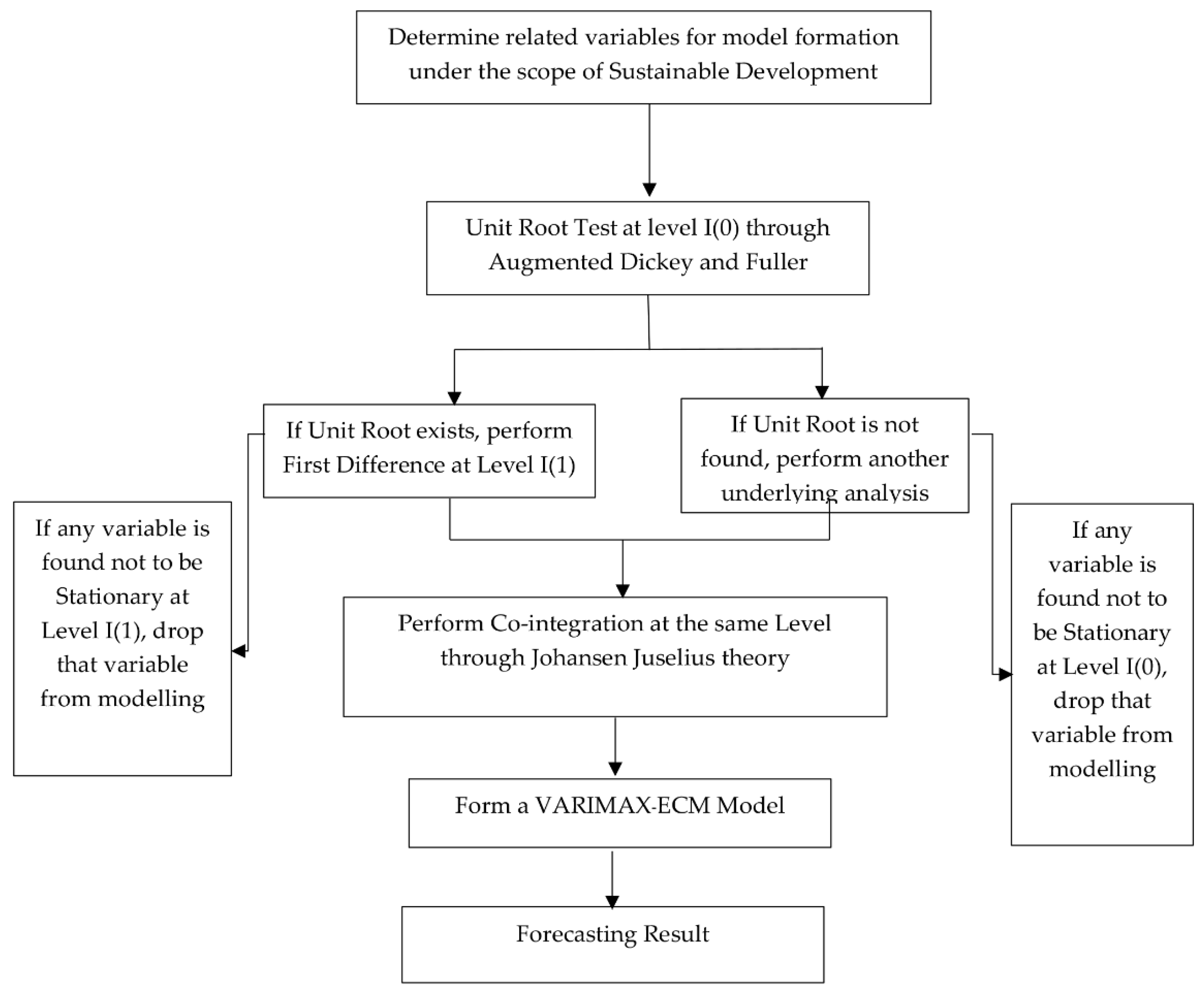
(1)

Analyze the causal variables that can influence the change of CO₂ emissions with the Augment Dickey Fuller theory [30] only at the same level. This analysis is within the framework of sustainable development, using data from 1990 to 2017. Moreover, only crucial and influential variables are used in the forecasting model.

(2)

Place the stationary causal variables at the same level in the analysis of long-term relationship based on the Johansen Juselius concept [31].

(3)

Create a forecasting model by adapting the advance statistics of the so-called vector autoregressive model, with full consideration of the relationship of all causal variables, both in terms of the error correction model and co-integration, consisting of significant causal variables towards the change of CO₂ emissions. Additionally, a forecasting pattern for both the short- and long-term must be taken into account so as to produce the best and most effective model with the least errors. The average relative errors between the simulation and actual data are measured through an output comparison of relevant models, namely the ARMA model, ARIMA model, and GM-ARIMA model.

(4)

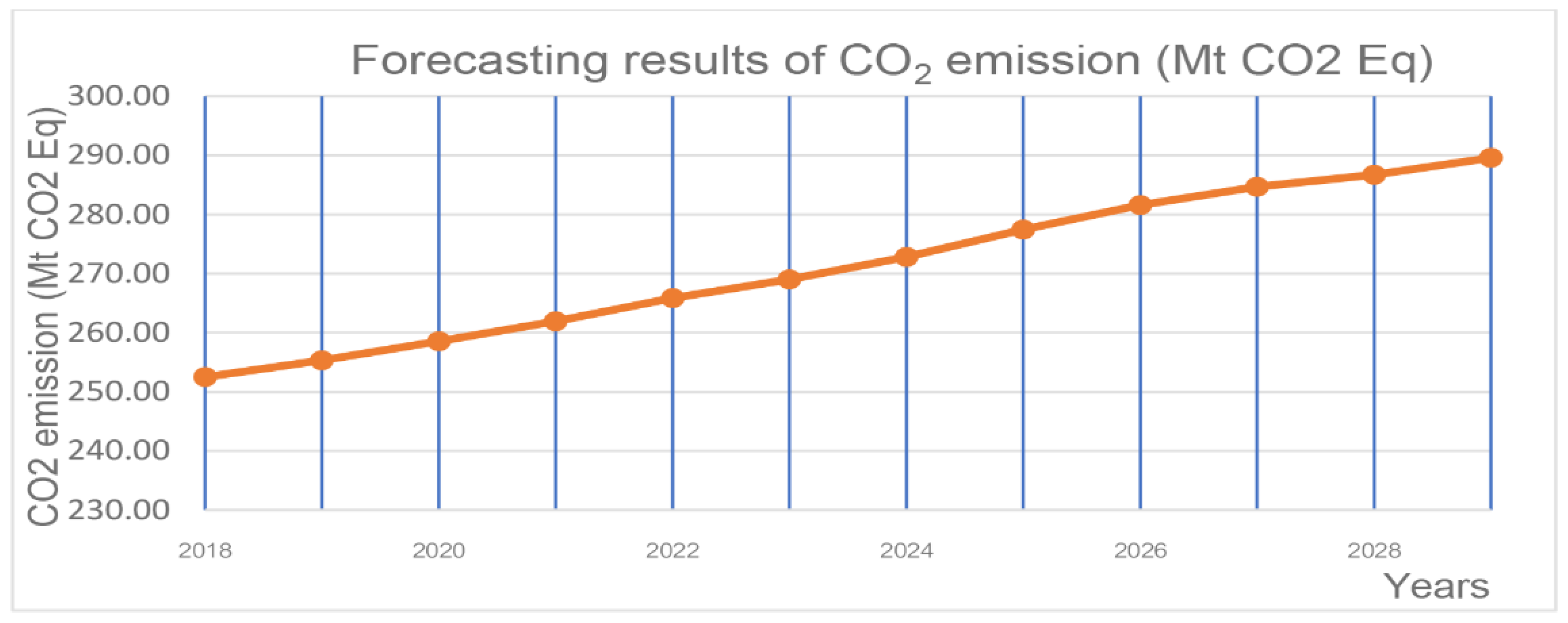
Forecast CO₂ emissions from the VARIMAX-ECM model for the period of 2018 to 2029, totaling 12 years, with certain selected causal factors. Discard unnecessary variables.

The flowchart of the VARIMAX-ECM model is shown in Figure 1.

The main structures of this article flow as follows: the second section introduces the forecasting model of VARIMAX-ECM. The third section carries out the empirical analysis to prove the practicality and validity of the proposed model for CO₂ emissions forecasting, and to predict the CO₂ emissions in Thailand’s industrial sector from 2018 to 2029. The fourth section summarizes the discussion.

2. The Forecasting Model

2.1. Unit Root Test

We analyze the data for the stationary process by testing the unit root according to the Augment Dickey Fuller concept [30].

Stationary Process

The stationary, or stationary stochastic, process [32,33] is the series of time data with the mean or expected value, variance, constant overtime, and covariance. The expected value and constant variance in the context of εt lacks the property of being white noise, meaning that it has the autocorrelation property where the correlations are high or the order of the autoregressive process is higher. Hence, a test like the Augmented Dickey Fuller test (ADF) is required. The lagged variables are added into the equation in the higher level to eliminate the autocorrelation, heteroskedasticity, and multicollinearity, as shown below:

$${\Delta \mathrm{Y}}_{\mathrm{t}}{=\mathsf{\delta }}_1{\mathrm{Y}}_{\mathrm{t}}+{\displaystyle \sum _{\mathrm{i}=2}^{\mathrm{p}}{\mathsf{\beta }}_{\mathrm{i}}{\Delta \mathrm{Y}}_{\mathrm{t}-\mathrm{i}+1}}{+\mathsf{\epsilon }}_{\mathrm{t}}$$

(1)

$${\Delta \mathrm{Y}}_{\mathrm{t}}{=\mathsf{\alpha }}_1{+\mathsf{\delta }}_{}{\mathrm{Y}}_{\mathrm{t}-1}+{\displaystyle \sum _{\mathrm{i}=2}^{\mathrm{p}}{\mathsf{\beta }}_{\mathrm{i}}{\Delta \mathrm{Y}}_{\mathrm{t}-\mathrm{i}+1}}{+\mathsf{\epsilon }}_{\mathrm{t}}$$

(2)

$${\Delta \mathrm{Y}}_{\mathrm{t}}{=\mathsf{\alpha }}_1{+\mathsf{\alpha }}_2{\mathrm{T}+\mathsf{\delta }}_{}{\mathrm{Y}}_{\mathrm{t}-1}+{\displaystyle \sum _{\mathrm{i}=2}^{\mathrm{p}}{\mathsf{\beta }}_{\mathrm{i}}{\Delta \mathrm{Y}}_{\mathrm{t}-\mathrm{i}+1}}{+\mathsf{\epsilon }}_{\mathrm{t}}$$

(3)

From the equations above, the value of p seems to be the lagged values of first difference to the variable, which is verified by testing the unit root with the Augmented Dickey Fuller method. With the above equation, three problems are considered and taken into account. In particular, the autocorrelation in ε_t is set to have the property of white noise, and the error term has the mean of 0 and is constant under the following hypotheses:

Hypotheses 1 (H₀).

δ = 0, non-stationary;

Hypotheses 2 (H₁).

δ < 0, stationary.

If tau-statistics of the efficiency δ are in the form of the absolute term, there must be more critical values appearing in the ADF table. This denies the major hypothesis, meaning that the time series of the variables are stationary. Thus, it can be said that ΔY_t integrated numbered is represented by ΔY_t ~ I(d).

2.2. VARIMAX-ECM Model

The VARIMAX-ECM model is a new model adapted from the vector autoregressive model, incorporating influential variables in both short-term and long-term relationships so as to produce the best prediction model with the maximum performance and least error.

2.2.1. VARIMAX-ECM and Co-Integrating Vector

In this section, we consider the segment of the deterministic component in a time series of the VAR model [34]. In order to simplify the concept for a better understanding, we consider the VAR model as follows:

$${\mathrm{X}}_{\mathrm{t}}{=\mathrm{A}}_1{\mathrm{X}}_{\mathrm{t}-1}{+\mathsf{\mu }}_0{+\mathsf{\mu }}_1{\mathrm{t}+\mathrm{u}}_{\mathrm{t}}$$

(4)

where ${\mathsf{\mu }}_0$ is the vector of the parameter representing a constant value in the VAR(p) model, ${\mathsf{\mu }}_1$ is the vector of the parameter indicating a defined trend in the VAR(p) model, and vectors ${\mathsf{\mu }}_0$ and ${\mathsf{\mu }}_1$ are shown below:

$${\mathsf{\mu }}_0={\left[\begin{array}{c}{\mathsf{\mu }}_{01}\\ {\mathsf{\mu }}_{02}\\ ⋮\\ {\mathsf{\mu }}_{0\mathrm{n}}\end{array}\right]}_{\mathrm{nx}1};{\mathsf{\mu }}_1={\left[\begin{array}{c}{\mathsf{\mu }}_{11}\\ {\mathsf{\mu }}_{12}\\ ⋮\\ {\mathsf{\mu }}_{1\mathrm{n}}\end{array}\right]}_{\mathrm{nx}1}$$

When vectors ${\mathsf{\mu }}_0$ and ${\mathsf{\mu }}_1$ are not zero, Equation (4) reflects that at least one time series in the VAR (1) model must be a deterministic component, in which it can either be a constant or a defined trend, or both forms. The above VAR(p) model can be converted into the VARIMAX-ECM model as shown below:

$${\Delta \mathrm{X}}_{\mathrm{t}}{=\mathsf{\alpha }\mathsf{\beta }}^{\prime }{\mathrm{X}}_{\mathrm{t}-1}{+\mathsf{\mu }}_0{+\mathsf{\mu }}_1{\mathrm{t}+\mathrm{u}}_{\mathrm{t}}$$

(5)

From the above equation, it can be observed that vectors ${\mathsf{\mu }}_0$ and ${\mathsf{\mu }}_1$ exist in both the VAR and VARIMAX–ECM models, and that both ${\Delta \mathrm{X}}_{\mathrm{t}}$ and ${\mathsf{\beta }}^{\prime }{\mathrm{X}}_{\mathrm{t}-1}$ have to be stationary in the deterministic area.

However, to observe a deviation out of the long-term co-integration of j (j = 1, 2, …, r) denoted as vector ${\mathsf{\beta }}^{\prime }{\mathrm{X}}_{\mathrm{t}-1}$, the mean of the above deviation must be zero. In order to obtain such a result, the deterministic component must be eliminated from the deviation out of long-term balance ${(\mathsf{\beta }}^{\prime }{\mathrm{X}}_{\mathrm{t}-1})$ by separating vectors ${\mathsf{\mu }}_0$ and ${\mathsf{\mu }}_1$ in the VARIMAX-ECM model, as illustrated in Equation (6), and by combining them into ${\mathsf{\beta }}^{\prime }{\mathrm{X}}_{\mathrm{t}-1}$ as explained below.

Vector ${\mathsf{\mu }}_0$ and vector ${\mathsf{\mu }}_1$ can be separated into the sum of the two vectors by using the following equation:

$${\mathsf{\alpha }(\mathsf{\beta }}^{\prime }{\mathsf{\alpha })}^{-1}{\mathsf{\beta }}^{\prime }{+\mathsf{\beta }}_{\perp }{{(\mathsf{\alpha }}^{\prime }{}_{\perp }{\mathsf{\beta }}_{\perp })}^{-1}{\mathsf{\alpha }}^{\prime }{}_{\perp }=\mathrm{I}$$

(6)

where ${\mathsf{\beta }}_{\perp }$ and ${\mathsf{\alpha }}_{\perp }$ are the orthogonal matrices with $\mathsf{\beta }$ and $\mathsf{\alpha }$, respectively. Here, it is seen that ${\mathsf{\beta }}^{\prime }{\mathsf{\beta }}_{\perp }=0$ and ${\mathsf{\alpha }}^{\prime }{\mathsf{\alpha }}_{\perp }=0$.

When we multiply vector ${\mathsf{\mu }}_0$ with Equation (6), the result is obtained from:

$${\mathsf{\alpha }(\mathsf{\beta }}^{\prime }{\mathsf{\alpha })}^{-1}{\mathsf{\beta }}^{\prime }{\mathsf{\mu }}_0{+\mathsf{\beta }}_{\perp }{{(\mathsf{\alpha }}^{\prime }{}_{\perp }{\mathsf{\beta }}_{\perp }^{})}^{-1}{\mathsf{\alpha }}^{\text{'}}{}_{\perp }{\mathsf{\mu }}_0{=\mathsf{\mu }}_0$$

(7)

If given:

$${\mathsf{\beta }}_0{=(\mathsf{\beta }}^{\prime }{\mathsf{\alpha })}^{-1}{\mathsf{\beta }}^{\prime }{\mathsf{\mu }}_0$$

(8)

$${\mathsf{\gamma }}_0{=\mathsf{\beta }}_{\perp }{{(\mathsf{\alpha }}^{\prime }{}_{\perp }{\mathsf{\beta }}_{\perp })}^{-1}{\mathsf{\alpha }}^{\prime }{}_{\perp }{\mathsf{\mu }}_0$$

(9)

We substitute Equations (8) and (9) into Equation (7), we obtain:

$${\mathsf{\mu }}_0{=\mathsf{\alpha }\mathsf{\beta }}_0{+\mathsf{\gamma }}_0$$

(10)

At the same time, if we use vector ${\mathsf{\mu }}_1$ to multiply with Equation (6), obtaining:

$${\mathsf{\mu }}_1{=\mathsf{\alpha }\mathsf{\beta }}_1{+\mathsf{\gamma }}_1$$

(11)

where ${\mathsf{\beta }}_1{=(\mathsf{\beta }}^{\prime }{\mathsf{\alpha })}^{-1}{\mathsf{\beta }}^{\prime }{\mathsf{\mu }}_1$ and ${\mathsf{\gamma }}_1{=\mathsf{\beta }}_{\perp }{{(\mathsf{\alpha }}^{\prime }{}_{\perp }{\mathsf{\beta }}_{\perp })}^{-1}{\mathsf{\alpha }}_1{\mathsf{\mu }}_1$.

If we substitute Equations (10) and (11) into Equation (5), we obtain:

$${\Delta \mathrm{X}}_{\mathrm{t}}^{}{=\mathsf{\alpha }\mathsf{\beta }}^{\prime }{\mathrm{X}}_{\mathrm{t}-1}{+\mathsf{\alpha }\mathsf{\beta }}_0{+\mathsf{\alpha }\mathsf{\beta }}_1{\mathrm{t}+\mathsf{\gamma }}_0{+\mathsf{\gamma }}_1{\mathrm{t}+\mathsf{\mu }}_{\mathrm{t}}$$

(12)

Equation (12) can be restructured as follows:

$${\Delta \mathrm{X}}_{\mathrm{t}}^{}{=\mathsf{\alpha }(\mathsf{\beta }}^{\prime }{\mathrm{X}}_{\mathrm{t}-1}{+\mathsf{\beta }}_0{+\mathsf{\beta }}_1{\mathrm{t})+\mathsf{\gamma }}_0{+\mathsf{\gamma }}_1{\mathrm{t}+\mathsf{\mu }}_{\mathrm{t}}$$

(13)

where ${\Delta \mathrm{X}}_{\mathrm{t}}^{}$ is the $n\times 1$ vector, ${\mathrm{X}}_{\mathrm{t}}^{}$ is the $n\times 1$ vector, $\mathsf{\alpha }$ is the $\mathrm{n}\times \mathrm{r}$ matrix, and $\mathsf{\beta }$ is the $\mathrm{n}\times \mathrm{r}$ matrix. ${\mathsf{\beta }}_0$ is the $\mathrm{r}\times 1$ matrix, ${\mathsf{\beta }}_1$ is the $\mathrm{r}\times 1$ matrix, ${\mathsf{\gamma }}_0$ is the $n\times 1$ matrix, ${\mathsf{\gamma }}_1$ is the $n\times 1$ matrix, and ${\mathsf{\mu }}_{\mathrm{t}}$ is the $n\times 1$ matrix. $\mathrm{n}$ is the number of time series in vector ${\mathrm{X}}_{\mathrm{t}}^{}$.

Equation (13) shows that if vector ${\mathrm{X}}_{\mathrm{t}}^{}$ determines ${(\mathsf{\mu }}_0{+\mathsf{\mu }}_1\mathrm{t})$, there is a possibility that the VARIMAX-ECM model determines ${(\mathsf{\gamma }}_0{+\mathsf{\gamma }}_1\mathrm{t})$ and the long-term co-integration determines ${(\mathsf{\beta }}_0{+\mathsf{\beta }}_1\mathrm{t})$. In addition, Equation (13) can be rewritten as:

$${\Delta \mathrm{X}}_{\mathrm{t}}^{}=\mathsf{\alpha }{\left[\begin{array}{ccc}{\mathsf{\beta }}^{\prime }& {\mathsf{\beta }}_0& {\mathsf{\beta }}_1^{}\end{array}\right]}_{\mathrm{r}\times (\mathrm{n}+2)}{\left[\begin{array}{c}{\mathrm{X}}_{\mathrm{t}-1}\\ 1\\ \mathrm{t}\end{array}\right]}_{(\mathrm{n}+2)\times 1}{+\mathsf{\gamma }}_0{+\mathsf{\gamma }}_1{\mathrm{t}+\mathsf{\mu }}_{\mathrm{t}}$$

(14)

Let ${\tilde{\mathsf{\beta }}}^{\prime }=\left[\begin{array}{ccc}{\mathsf{\beta }}^{\prime }& {\mathsf{\beta }}_0& {\mathsf{\beta }}_1^{}\end{array}\right]$, ${\tilde{\mathrm{X}}}_{\mathrm{t}-1}={\left[\begin{array}{ccc}{\mathrm{X}}_{\mathrm{t}-1}& 1& \mathrm{t}\end{array}\right]}^{\prime }$, and we can then structure another equation as:

$${\Delta \mathrm{X}}_{\mathrm{t}}{=\mathsf{\alpha }\tilde{\mathsf{\beta }}}^{\prime }{\tilde{\mathrm{X}}}_{\mathrm{t}-1}{+\mathsf{\gamma }}_0{+\mathsf{\gamma }}_1{\mathrm{t}+\mathrm{u}}_{\mathrm{t}}^{}$$

(15)

The above equation contains the following characteristics:

$${\mathrm{E}(\Delta \mathrm{X}}_{\mathrm{t}}{)=\mathsf{\gamma }}_0{+\mathsf{\gamma }}_1\mathrm{t};{\mathrm{E}(\tilde{\mathsf{\beta }}}^{\prime }{\tilde{\mathrm{X}}}_{\mathrm{t}-1})=0$$

(16)

Moreover, Equation (15) explains the connection between the deterministic area of the VARIMAX-ECM model and the long-term co-integrating vector, which can be classified into five situations.

Situation 1: If ${\mathsf{\gamma }}_0{=\mathsf{\gamma }}_1{=\mathsf{\beta }}_0$ or (${\mathsf{\mu }}_0{=\mathsf{\mu }}_1=0$) for both the VARIMAX-ECM model and the long-term co-integrating vector (deviation out of long-term balance), they are not deterministic or can be expressed as ${\mathrm{E}(\Delta \mathrm{X}}_{\mathrm{t}})=0$ and ${\mathrm{E}(\mathsf{\beta }}^{\prime }{\tilde{\mathrm{X}}}_{\mathrm{t}-1})=0$. Therefore, the VARIMAX-ECM model in this position is:

$${\Delta \mathrm{X}}_{\mathrm{t}}{=\mathsf{\alpha }\mathsf{\beta }}^{\prime }{\mathrm{X}}_{\mathrm{t}-1}{+\mathrm{u}}_{\mathrm{t}}$$

(17)

The case of ${\mathsf{\mu }}_0{=\mathsf{\mu }}_1=0$ indicates a time series in vector ${\mathrm{X}}_{\mathrm{t}}$ and is not deterministic (it is not constant nor a defined trend) in the equation.

Situation 2: If ${\mathsf{\gamma }}_0=0$, ${\mathsf{\gamma }}_1{=\mathsf{\beta }}_1=0$ (or ${\mu }_1=0$) but ${\mathsf{\beta }}_0\ne 0$, then the vector of the long-term co-integration reflects a constant value (${\mathsf{\beta }}_0\ne 0$) or can be written as ${\mathrm{E}(\mathsf{\beta }}^{\prime }{\mathrm{X}}_{\mathrm{t}-1}{)=\mathsf{\beta }}_0$. Meanwhile, the VARIMAX-ECM model is not deterministic at all, or can be written as ${\mathrm{E}(\Delta \mathrm{X}}_{\mathrm{t}})=0$. In order to remove the constant value out of the long-term co-integration, the VARIMAX-ECM model must be in the form of:

$${(\Delta \mathrm{X}}_{\mathrm{t}}{)=\mathsf{\alpha }\tilde{\mathsf{\beta }}}^{\prime }{\tilde{\mathrm{X}}}_{\mathrm{t}-1}{+\mathrm{u}}_{\mathrm{t}}$$

(18)

where ${\tilde{\mathsf{\beta }}}^{\prime }=\left[\begin{array}{cc}{\mathsf{\beta }}^{\prime }& {\mathsf{\beta }}_0\end{array}\right]$ and ${\tilde{\mathrm{X}}}_{\mathrm{t}-1}={\left[\begin{array}{cc}{\mathrm{X}}_{\mathrm{t}-1}& 1\end{array}\right]}^{\prime }$. Thus, we can retrieve ${\mathrm{E}(\tilde{\mathsf{\beta }}}^{\prime }{\tilde{\mathrm{X}}}_{\mathrm{t}-1})=0$.

The case of ${\mathsf{\mu }}_1=0$ and ${\mathsf{\gamma }}_0=0$, but ${\mathsf{\beta }}_0\ne 0$, indicates at least one time series in vector ${\mathrm{X}}_{\mathrm{t}}$ and is constant (but it is not a defined trend) in the equation.

Situation 3: If ${\mathsf{\gamma }}_1{=\mathsf{\beta }}_1=0$ (or ${\mathsf{\mu }}_1=0$) but ${\mathsf{\gamma }}_0\ne 0$ and ${\mathsf{\beta }}_0\ne 0$, the vector of the long-term co-integration is not a defined trend but is constant (${\mathsf{\beta }}_0\ne 0$), or can be written as ${\mathrm{E}(\mathsf{\beta }}^{\prime }{\mathrm{X}}_{\mathrm{t}-1}{)=\mathsf{\beta }}_0$. If the VARIMAX-ECM model is found to be constant, ${\mathsf{\gamma }}_0\ne 0$, or can be written as ${\mathrm{E}(\Delta \mathrm{X}}_{\mathrm{t}}{)=\mathsf{\gamma }}_0$, and the above fixed value in the long-term co-integrating vector can be removed by using the long-term co-integration ${\tilde{\mathsf{\beta }}}^{\prime }{\tilde{\mathrm{X}}}_{\mathrm{t}-1}$ in the VARIMAX-ECM model, as illustrated below:

$${\Delta \mathrm{X}}_{\mathrm{t}}{=\mathsf{\alpha }\tilde{\mathsf{\beta }}}^{\prime }{\tilde{\mathrm{X}}}_{\mathrm{t}-1}{+\mathsf{\gamma }}_0{+\mathrm{u}}_{\mathrm{t}}$$

(19)

where ${\tilde{\mathsf{\beta }}}^{\prime }=\left[\begin{array}{cc}{\mathsf{\beta }}^{\prime }& {\mathsf{\beta }}_0\end{array}\right]$ and ${\tilde{\mathrm{X}}}_{\mathrm{t}-1}={\left[\begin{array}{cc}{\mathrm{X}}_{\mathrm{t}-1}& 1\end{array}\right]}^{\prime }$.

The case of ${\mathsf{\mu }}_1=0$, but ${\mathsf{\gamma }}_0\ne 0$ and ${\mathsf{\beta }}_0\ne 0$ indicates that at least one time series is a defined trend.

Situation 4: If ${\mathsf{\gamma }}_1=0$, but ${\mathsf{\gamma }}_0\ne 0$, ${\mathsf{\beta }}_0\ne 0$ (or ${\mathsf{\mu }}_0\ne 0$), and ${\mathsf{\beta }}_0\ne 0$, the long-term co-integration ${\mathsf{\beta }}^{\prime }{\mathrm{X}}_{\mathrm{t}-1}$ cannot eliminate the constant value and defined trend, and it can be rewritten as ${\mathrm{E}(\mathsf{\beta }}^{\prime }{\mathrm{X}}_{\mathrm{t}-1}{)=\mathsf{\beta }}_0{+\mathsf{\beta }}_1\mathrm{t}$. This can be described in such a way that the long-term co-integration is a stationary trend, while the VARIMAX-ECM model is found to have a fixed value of ${\mathsf{\gamma }}_0\ne 0$ or can be written as ${\mathrm{E}(\Delta \mathrm{X}}_{\mathrm{t}}{)=\mathsf{\gamma }}_0$. The fixed value and defined trend that exist in the long-term co-integrating vector could be removed by using a ${\tilde{\mathsf{\beta }}}^{\prime }{\tilde{\mathrm{X}}}_{\mathrm{t}-1}$ long-term co-integration in the VARIMAX-ECM model as follows:

$${\Delta \mathrm{X}}_{\mathrm{t}}{=\mathsf{\alpha }\tilde{\mathsf{\beta }}}^{\prime }{\tilde{\mathrm{X}}}_{\mathrm{t}-1}{+\mathsf{\gamma }}_0{+\mathrm{u}}_{\mathrm{t}}$$

(20)

where ${\tilde{\mathsf{\beta }}}^{\prime }=\left[\begin{array}{ccc}{\mathsf{\beta }}^{\prime }& {\mathsf{\beta }}_0& {\mathsf{\beta }}_1^{}\end{array}\right]$ and ${\tilde{\mathrm{X}}}_{\mathrm{t}-1}=\left[\begin{array}{c}{\mathrm{X}}_{\mathrm{t}-1}\\ 1\\ \mathrm{t}\end{array}\right]$ , which can also be written as ${\left[\begin{array}{ccc}{\mathrm{X}}_{\mathrm{t}-1}& 1& \mathrm{t}\end{array}\right]}^{\prime }$.

The case of ${\mathsf{\mu }}_1\ne 0$ and ${\mathsf{\gamma }}_1=0$ but ${\mathsf{\beta }}_1\ne 0$ demonstrates that at least one time series in vector ${\mathrm{X}}_{\mathrm{t}}$ has to be constant and a defined linear trend, but it is not a quadratic trend.

Situation 5: If ${\mathsf{\gamma }}_1\ne 0$, ${\mathsf{\gamma }}_0\ne 0$, ${\mathsf{\beta }}_0\ne 0$, and ${\mathsf{\beta }}_0\ne 0$, this shows that the long-term co-integration has to be a stationary trend ${(\mathsf{\beta }}_0{+\mathsf{\beta }}_1\mathrm{t})$, while the VARIMAX-ECM model has to be constant and defined trend ${(\mathsf{\gamma }}_0{+\mathsf{\gamma }}_1\mathrm{t})$ which can be written as below:

$${\Delta \mathrm{X}}_{\mathrm{t}}{=\mathsf{\alpha }\tilde{\mathsf{\beta }}}^{\prime }{\tilde{\mathrm{X}}}_{\mathrm{t}-1}{+\mathsf{\gamma }}_0{+\mathsf{\gamma }}_1{\mathrm{t}+\mathrm{u}}_{\mathrm{t}}$$

(21)

where ${\tilde{\mathsf{\beta }}}^{\prime }=\left[\begin{array}{ccc}{\mathsf{\beta }}^{\prime }& {\mathsf{\beta }}_0& {\mathsf{\beta }}_1^{}\end{array}\right]$ and ${\tilde{\mathrm{X}}}_{\mathrm{t}-1}={\left[\begin{array}{ccc}{\mathrm{X}}_{\mathrm{t}-1}& 1& \mathrm{t}\end{array}\right]}^{\prime }{}^{}$. The case of ${\mathsf{\mu }}_0\ne 0$ and ${\mathsf{\mu }}_1\ne 0$ occurs when at least one time series in vector X_t has to be defined by a quadratic trend ${(\mathsf{\mu }}_0{+\mathsf{\mu }}_1{\mathrm{t}+\mathsf{\mu }}_2{\mathrm{t}}^2)$.

2.2.2. An Estimation of the Co-Integrating Vector with the Use of Various Equations [33]

Consider the VARIMAX-ECM model as follows [35]:

$${\Delta \mathrm{X}}_{\mathrm{t}}{=\mathsf{\alpha }\tilde{\mathsf{\beta }}}^{\prime }{\tilde{\mathrm{X}}}_{\mathrm{t}-1}{+\mathsf{\Gamma }}_1{\Delta \mathrm{X}}_{\mathrm{t}-1}{+\mathsf{\Gamma }}_2{\Delta \mathrm{X}}_{\mathrm{t}-2}+\dots {+\mathsf{\Gamma }}_{\mathrm{p}-1}{\Delta \mathrm{X}}_{\mathrm{t}-(\mathrm{p}-1)}{+\mathsf{\phi }\mathrm{D}}_{\mathrm{t}}{+\mathrm{u}}_{\mathrm{t}}$$

(22)

where ${\tilde{\mathsf{\beta }}}^{\prime }=\left[\begin{array}{ccc}{\mathsf{\beta }}^{\prime }& {\mathsf{\beta }}_0& {\mathsf{\beta }}_1^{}\end{array}\right]$ is the $\mathrm{r}\times (\mathrm{n}+2)$ matrix, $\mathsf{\beta }$ is the $\mathrm{n}\times \mathrm{r}$ matrix, ${\mathsf{\beta }}_0$ and ${\mathsf{\beta }}_1$ are the $\mathrm{r}\times 1$ vector, ${\tilde{\mathrm{X}}}_{\mathrm{t}-1}={\left[\begin{array}{ccc}{\mathrm{X}}_{\mathrm{t}-1}& 1& \mathrm{t}\end{array}\right]}^{\prime }{}^{}$ is the $(\mathrm{n}+2)\times 1$ vector, $\mathsf{\alpha }$ is the $\mathrm{n}\times \mathrm{r}$ matrix, and rank ($\mathsf{\alpha }$) = rank $\left(\tilde{\mathsf{\beta }}\right)=\mathrm{r}$. Additionally, ${\mathrm{D}}_{\mathrm{t}}$ is the matrix indicating a deterministic component.

The estimation of the parameter of the long-term co-integrating vector $\tilde{\mathsf{\beta }}$ can be achieved with the application of maximum likelihood by assuming vector ${\mathrm{u}}_{\mathrm{t}}^{}\approx$ Normal (0, $\sum$) 0 is zero, and $\sum$ is the variant matrix of ${\mathrm{u}}_{\mathrm{t}}$. Johansen (1995) proved that the estimation of vector ${\tilde{\mathsf{\beta }}}_{\mathrm{n}\times \mathrm{r}}$ with this method would result in an eigenvector in accordance with the eigenvalue from the minimum to maximum value. This is achieved using the equation below:

$$\left|\mathsf{\lambda }{\mathrm{S}}_{11}-{\mathrm{S}}_{10}{\mathrm{S}}_{00}^{-1}{\mathrm{S}}_{01}\right|=0$$

(23)

${\mathrm{S}}_{\mathrm{ij}}=\frac{1}{\mathrm{T}}{\mathrm{R}}_{\mathrm{it}}{\mathrm{R}}_{\mathrm{jt}}^{\prime }$, $\mathrm{i}=0,1$, and $\mathrm{j}=0,1$; where $\mathrm{T}$ is the number of data used in the VARIMAX-ECM model. ${\mathrm{R}}_{0\mathrm{t}}$ is the $\mathrm{n}\times \mathrm{T}$ matrix of the residual retrieved from a regression equation with a variable of ${\Delta \mathrm{X}}_{\mathrm{t}}$, and the independent variable is ${\Delta \mathrm{X}}_{\mathrm{t}-1}$, ${\Delta \mathrm{X}}_{\mathrm{t}-2}$,…, ${\Delta \mathrm{X}}_{\mathrm{t}-\mathrm{p}+1}$, ${\mathrm{D}}_{\mathrm{t}}$. ${\mathrm{R}}_{1\mathrm{t}}$ is the $(\mathrm{n}+2)\times \mathrm{T}$ matrix of the residual retrieved from a regression equation with a variable of ${\tilde{\mathrm{X}}}_{\mathrm{t}-1}$, and the independent variable is ${\Delta \mathrm{X}}_{\mathrm{t}-1}$, ${\Delta \mathrm{X}}_{\mathrm{t}-2}$,…, ${\Delta \mathrm{X}}_{\mathrm{t}-\mathrm{p}+1}$, ${\mathrm{D}}_{\mathrm{t}}$.

If ${\hat{\mathsf{\lambda }}}_{\mathrm{i}}{(\mathrm{i}=1,2,\dots ,\mathrm{n})}^{11}$ is the eigenvalue computed from Equation (24) where $1$ > ${\hat{\mathsf{\lambda }}}_1$ > ${\hat{\mathsf{\lambda }}}_2$ > … > ${\hat{\mathsf{\lambda }}}_{\mathrm{n}}$ $\ge 0$, let the eigenvector consistant with the eigenvalue ${\hat{\mathsf{\lambda }}}_1$, ${\hat{\mathsf{\lambda }}}_2$, …, ${\hat{\mathsf{\lambda }}}_{\mathrm{n}}$ be written as $\hat{\mathrm{V}}={\left[\begin{array}{cccc}{\hat{\mathrm{V}}}_1& {\hat{\mathrm{V}}}_2& \dots & {\hat{\mathrm{V}}}_{\mathrm{n}}\end{array}\right]}_{(n+2)\times (n+2)}$. Therefore, we can obtain the estimator of the co-integrating vector as follows:

$$\hat{\mathrm{V}}={\left[\begin{array}{cccc}{\hat{\mathrm{V}}}_1& {\hat{\mathrm{V}}}_2& \dots & {\hat{\mathrm{V}}}_{\mathrm{r}}\end{array}\right]}_{(n+2)\times r}$$

(24)

Commonly, there are two popular patterns of forming primary and secondary assumptions pertaining to the number of the long-term co-integration.

Pattern 1: H₀ is the maximal number of vectors indicating the long-term co-integration equivalent to r. H₁ is the number of vectors indicating the long-term co-integration greater than r.

In the above, $\mathrm{r}=\begin{array}{cccc}0,& 1,& 2,& \dots ,\end{array}\mathrm{n}-1$, and the statistical value to testify the above assumption is trace statistic ${\mathsf{\lambda }}_{\mathrm{trace}}$, which can be computed using the equation below:

$${\mathsf{\lambda }}_{\mathrm{trace}}(\mathrm{r})=-\mathrm{T}{\displaystyle \sum _{\mathrm{i}=\mathrm{r}+1}^{\mathrm{n}}(1-{\hat{\mathsf{\lambda }}}_{\mathrm{i}})}$$

(25)

Pattern 2:${\mathrm{H}}_0$ is the maximal number of vectors indicating the long-term co-integration equivalent to r. ${\mathrm{H}}_1$ is the number of vectors indicating the long-term co-integration equivalent to $\mathrm{r}+1$.

In the above, $\mathrm{r}=\begin{array}{cccc}0,& 1,& 2,& \dots ,\end{array}\mathrm{n}-1$, and the statistical value to testify the above assumption is maximum eigenvalue ${\mathsf{\lambda }}_{\mathrm{trace}}$, which can be computed using the equation below:

$${\mathsf{\lambda }}_{\max }(\mathrm{r},\mathrm{r}+1)=-\mathrm{T}(1-{\hat{\mathsf{\lambda }}}_{\mathrm{r}+1})$$

(26)

$${\hat{\mathrm{A}}}_{\mathrm{i}}=\{\begin{array}{c}\mathrm{I}+\stackrel{⌢}{\mathsf{\Pi }}+\stackrel{⌢}{\mathsf{\Gamma }}\\ {\stackrel{⌢}{\mathsf{\Gamma }}}_{\mathrm{i}}-{\stackrel{⌢}{\mathsf{\Gamma }}}_{\mathrm{i}-1}\\ -{\stackrel{⌢}{\mathsf{\Gamma }}}_{\mathrm{p}-1}\end{array}\begin{array}{c},i=1\\ ,2\le i\le -1\\ ,i=p\end{array}$$

(27)

After that, we use the VARIMAX-ECM forecasting model of the time series in vector ${\mathrm{X}}_{\mathrm{t}}$ by using the same concept, which is the forecasting of the minimum mean square error. Hence, the forecast of $1,2,\dots ,\mathrm{h}$ pre-timing of the time series in the vector ${\mathrm{X}}_{\mathrm{t}}$ can be illustrated as:

$${\hat{\mathrm{X}}}_{\mathrm{T}+1}{=\hat{\mathrm{A}}}_1{\mathrm{X}}_{\mathrm{T}}{+\hat{\mathrm{A}}}_2{\mathrm{X}}_{T-1}{+\hat{\mathrm{A}}}_{\mathrm{p}}{\mathrm{X}}_{T-p+1}$$

(28)

$${\hat{\mathrm{X}}}_{\mathrm{T}+2}{=\hat{\mathrm{A}}}_1{\mathrm{X}}_{\mathrm{T}+1}{+\hat{\mathrm{A}}}_2{\mathrm{X}}_{T-1}{+\hat{\mathrm{A}}}_{\mathrm{p}}{\mathrm{X}}_{T-p+2}$$

(29)

$${\hat{\mathrm{X}}}_{\mathrm{T}+\mathrm{h}}{=\hat{\mathrm{A}}}_1{\mathrm{X}}_{T+h-1}{+\hat{\mathrm{A}}}_2{\mathrm{X}}_{T+h-2}+\dots +{\hat{\mathrm{A}}}_{\mathrm{p}}{\mathrm{X}}_{T-p+h}$$

(30)

where ${\hat{\mathrm{X}}}_{\mathrm{T}+\mathrm{j}}{=\hat{\mathrm{A}}}_1{\mathrm{X}}_{\mathrm{T}+\mathrm{j}}$ if $\mathrm{j}<0$.

2.2.3. Measurement of the Forecasting Performance

In order to evaluate the forecasting effect of each model, we employ the mean absolute percentage error (MAPE) to compare the forecasting accuracy of each model. The calculated equations are shown as follows:

$$\mathrm{MAPE}=\frac{1}{\mathrm{n}}{\displaystyle \sum _{\mathrm{i}=1}^{\mathrm{n}}\left|\frac{{\hat{\mathrm{y}}}_{\mathrm{i}}-{\mathrm{y}}_{\mathrm{i}}}{{\mathrm{y}}_{\mathrm{i}}}\right|}$$

(31)

3. Empirical Analysis

3.1. Screening of Influencing Factors for Model Input

In this paper, we tested the causal factors in the context of Thailand’s sustainable development policy. Here, we deploy the time series data of the period of 1990–2017. The tested factors consist of seven variables, namely CO₂ emission (${\ln (\mathrm{CO}}_2)$), population growth ($\ln \left(\mathrm{Population}\right)$), per capita GDP ($\ln \left(\mathrm{GDP}\right)$), urbanization rate ($\ln \left(\mathrm{UR}\right)$), industrial structure ($\ln \left(\mathrm{IS}\right)$), total coal consumption ($\ln \left(\mathrm{CC}\right)$), and total exports and imports ($\ln (\mathrm{X}-\mathrm{E})$). The test was conducted based on the Augment Dickey Fuller theory at Level I (0) and Fist Difference I (1), as illustrated in

Table 1. Unit root test at Level I (0) and First Difference I (1).

ADF Test at Level I (0)		ADF Test at First Difference I (1)		MacKinnon Critical Value
				1%	5%	10%
${\ln (\mathrm{CO}}_2)$	−3.41	${\Delta \ln (\mathrm{CO}}_2)$	−4.90	−4.12	−3.27	−3.05
$\ln \left(\mathrm{Population}\right)$	−2.05	$\Delta \ln \left(\mathrm{Population}\right)$	−3.02	−4.12	−3.27	−3.05
$\ln \left(\mathrm{GDP}\right)$	−3.81	$\Delta \ln \left(\mathrm{GDP}\right)$	−5.69	−4.12	−3.27	−3.05
$\ln \left(\mathrm{UR}\right)$	−3.25	$\Delta \ln \left(\mathrm{UR}\right)$	−4.71	−4.12	−3.27	−3.05
$\ln \left(\mathrm{IS}\right)$	−3.72	$\Delta \ln \left(\mathrm{IS}\right)$	−4.65	−4.12	−3.27	−3.05
$\ln \left(\mathrm{CC}\right)$	−2.45	$\Delta \ln \left(\mathrm{CC}\right)$	−3.01	−4.12	−3.27	−3.05
$\ln (\mathrm{X}-\mathrm{E})$	−3.64	$\Delta \ln (\mathrm{X}-\mathrm{E})$	−4.64	−4.12	−3.27	−3.05

Note: ${\ln (\mathrm{CO}}_2)$ is the natural logarithm of CO₂ emissions; $\ln \left(\mathrm{Population}\right)$ is the natural logarithm of population growth; $\ln \left(\mathrm{GDP}\right)$ is the natural logarithm of per capita GDP; $\ln \left(\mathrm{UR}\right)$ is the natural logarithm of urbanization rate; $\ln \left(\mathrm{IS}\right)$ is the natural logarithm of industrial structure; $\ln \left(\mathrm{CC}\right)$ is the natural logarithm of total coal consumption; $\ln (\mathrm{X}-\mathrm{E})$ is the natural logarithm of total exports and imports, and $\Delta$ is the first difference.

.

Table 1 shows that all variables under the unit root test are non-stationary at Level I (0), and this explains the non-significance at 5% and 1%. Therefore, the First Difference I (1) is required to carry on. The finding here indicates that when the variables are tested through the unit root test at Level I (1) with a significance level of 5% and 1%, or stationary identification, the variables appear to be CO₂ emissions, per capita GDP, urbanization rate, industrial structure, and total exports and imports. Thus, these variables are carried forward for a co-integration analysis. The other two variables, population growth and total coal consumption, are non-stationary at Level I (1). Therefore, the researcher tests the two variables in pairs with other variables. The outcome shows that the variables do not represent any correlation to the changes in CO₂ emissions at significance levels of 5% and 1%. Accordingly, the two variables are dropped out of the model. Meanwhile, those stationary variables at the First Difference are brought forth to investigate the long-term relationship (co-integration) as demonstrated in

Table 2. Co-integration test by Johansen Juselius.

Variables	Hypothesized No of CE(S)	Trace Statistic Test	MacKinnon Critical Value		Max-Eigen Statistic Test	MacKinnon Critical Value		Status
			1%	5%		1%	5%
${\Delta \ln (\mathrm{CO}}_2)$, $\Delta \ln \left(\mathrm{GDP}\right)$, $\Delta \ln \left(\mathrm{UR}\right)$, $\Delta \ln \left(\mathrm{IS}\right)$, $\Delta \ln (\mathrm{X}-\mathrm{E})$	None **	210.25	19.75	15.41	130.55	15.68	14.07	I (1)
	At Most 1 **	70.55	5.75	3.16	75.46	5.75	3.16	I (1)

** denotes significance α = 0.01.

.

3.2. Analysis of Co-Integration

Table 2 shows that all variables have a long-term relationship (co-integration), because the results of the trace test are 210.25 and 70.55, which are higher than the critical values at significance levels of 1% and 5%. The maximum eigenvalue test results are 130.55 and 75.46, which are higher than the critical values at the same significance levels. Consequently, those variables are used to form a forecasting model by adapting the ARIMAX-ECM model and applying short- and long-term relationships into the model. For a better understanding, the model is presented in the form of a regression line, so as to show the influence of variables as seen in

Table 3. The result of the VARIMAX-ECM model.

Dependent Variables	Direction of Causality
	Short Term					Long Term
	${\displaystyle \sum {\mathsf{\Delta }\mathbf{ln}(\mathbf{CO}}_2)}$	${\displaystyle \sum \mathsf{\Delta }\mathbf{ln}\left(\mathbf{GDP}\right)}$	${\displaystyle \sum \mathsf{\Delta }\mathbf{ln}\left(\mathbf{UR}\right)}$	${\displaystyle \sum \mathsf{\Delta }\mathbf{ln}\left(\mathbf{IS}\right)}$	${\displaystyle \sum \mathsf{\Delta }\mathbf{ln}(\mathbf{X}-\mathbf{E})}$	${\mathbf{ECM}}_{\mathbf{t}-1}$
${\Delta \ln (\mathrm{CO}}_2)$		6.43 **	4.76 **	3.42 **	5.13 **	−2.15 **
$\Delta \ln \left(\mathrm{GDP}\right)$	4.31 *		3.05 **	5.77 **	6.65 **	−2.05 **
$\Delta \ln \left(\mathrm{UR}\right)$	3.76 *	3.44 *		6.59 **	4.61 **	−1.97 **
$\Delta \ln \left(\mathrm{IS}\right)$	4.71 **	2.78 *	3.49 **		7.11 **	−1.51 **
$\Delta \ln (\mathrm{X}-\mathrm{E})$	2.45 *	2.98 **	6.78 **	4.62 **		−2.77 **

In the above, ** denotes significance α = 0.01, * denotes significance α = 0.05, R-squared is 0.92, adjusted R-squared is 0.91, the Durbin-Watson statistic is 2.02, the F-statistic is 275.05 (probability is 0.00), the ARCH test is 30.45 (probability is 0.1), the LM test is 1.55 (probability is 0.10), and the response test (${\mathsf{\chi }}^2>\mathrm{critical}$) represents the significance.

.

3.3. Formation of Analysis Modeling with the VARIMAX-ECM Model

Table 3 illustrates the parameters of the VARIMAX-ECM Model at a statistically significant level of 1% and 5%. The findings show that per capita GDP ($\ln \left(\mathrm{GDP}\right)$) causes a change in CO₂ emissions (${\ln (\mathrm{CO}}_2)$), which covers both short- and long-terms at a statistically significant level of 1%. At the same significant level and effect coverage, the urbanization rate ($\ln \left(\mathrm{UR}\right)$), total coal consumption ($\ln \left(\mathrm{CC}\right)$) and total exports and imports ($\ln (\mathrm{X}-\mathrm{E})$) are also found to cause changes in CO₂ emissions (${\ln (\mathrm{CO}}_2)$). Hence, this study suggests that the above causal factors have an influence over changes in CO₂ emissions with the parameter size shown in the table.

However, this study also reveals that the changes in per capita GDP ($\ln \left(\mathrm{GDP}\right)$), urbanization rate ($\ln \left(\mathrm{UR}\right)$), total coal consumption, and total exports and imports ($\ln (\mathrm{X}-\mathrm{E})$) are caused by the factors shown in

Table 4. The performance monitoring of the forecasting model.

Forecasting Model	MAPE (%)
ARMA Model	7.44
ARIMA Model	5.75
GM-ARIMA Model	2.25
VARIMAX-ECM Model	1.01

at a statistically significant level of 1% and 5%, respectively, for both short- and long-terms with the parameter size stated in the table.

In addition to this, the author has compared some selected forecasting models in terms of their effectiveness with MAPE as indicated in Table 4. The comparison takes the VARIMAX-ECM model compared with other models, including the ARMA model, ARIMA model, and GM-ARIMA model, as follows.

Table 4 shows that the VARIMAX-ECM model has the lowest MAPE value at 1.01%. Accordingly, the GM-ARIMA model, ARIMA model, and ARMA model have MAPE values of 2.25%, 5.75%, and 7.44%, respectively. Based on the findings of the study, it has shown that the VARIMAX-ECM model used by the author is the most effective one. This can be observed from the value of the mean absolute percentage error (MAPE) was found to be lowest compared to the old model. Moreover, the study has also found that the VARIMAX-ECM model is suitable for long-term forecasting unlike other previously conducted studies, which were mostly old models proved only to be feasible for short-term forecasting. In addition to this, the VARIMAX-ECM model is a forecasting model which captures, with detail and prudency in the analysis process, by selecting the only stationary causal variables at the same level, as well as securing the same level of co-integration in order to create the best model. If any of the variables does not meet the set conditions, it would not be taken into account. Therefore, the VARIMAX-ECM model becomes the right forecasting model suitable for long-term policy-making and management planning in order to achieve a sustainable development in the future. Therefore, the VARIMAX-ECM model is used to forecast CO₂ emissions in the following step.

3.4. CO₂ Emissions Forecasting Based on the VARIMAX-ECM Model

Figure 2 shows that CO₂ emissions from 2018 to 2029 in Thailand are continuously increasing with changes up to 14.68% or 289.58 Mt CO₂ Eq. The result shown is beyond the target and deviates from the reduction policy; CO₂ emissions are expected to reduce by 20.8%, or be less than 115 Mt CO₂ Eq. in the industrial sectors so as to attain sustainable development.

4. Conclusions and Discussion

This study disclosed new knowledge and guidelines for future research. The forecasting model must emphasize the causal factors that can influence CO₂ emissions in both the short- and long-term. In addition, the to-be-used variables must be stationary at the same level. It is important to drop or ignore unnecessary variables, which have no direct influence on the dependent variables, so as to produce the best performing model with the most effective prediction outcomes. At the same time, this will facilitate the formulation of effective sustainable development policies. The newly-introduced model in this study attempts to fill the gaps or weaknesses of most existing forecasting models. Additionally, it provides more accurate output with fewer errors, which is instrumental for both the academic world and the country in enhancing policy-making for future sustainable development.

From this study’s findings, both the short- and long-term causal factors affecting CO₂ emissions are per capita GDP, urbanization rate, industrial structure, and total exports and imports. These variables can be employed to formulate the VARIMAX-ECM model through a performance testing based on MAPE values. Here, the test’s results indicate this model’s higher quality and efficiency compared to other existing models, such as the ARMA, ARIMA, and GM-ARIMA models. This illustrates that the VARIMAX-ECM model is one of the best models suitable for the future forecasting of CO₂ emissions. Deploying the data of 2018 to 2029, we found that CO₂ emissions continue to increase by 14.68%, which is not in line with Thailand’s reduction policy, in which Thailand aims to reduce CO₂ emissions to be lower than 20.8% by 2029.

This study produced new findings and, thus, differentiates itself from other existing studies, including those studies in the above literature review. Specifically, this study generated a forecasting model with the ability to provide a long-term forecast over more than 10 years (2018–2029) and perform effectively. In addition, this study is one of the first reports to introduce the VARIMAX-ECM model. This model is basically adapted from the existing concept and theory. Based on previous studies, the VARIMAX-ECM model is the best model appropriate for long-term forecasting. Unlike many existing and relevant studies, this study makes long-term forecasting possible. This can be observed from the review of relevant studies with the capability of only short-term prediction. For instance, Dai, Niu, and Han [28] put forth the GM (grey model) and least squares support vector machine (LSSVM), along with the optimization of the modified shuffled frog-leaping algorithm (MSFLA) (MSFLA-LSSVM), to forecast CO₂ emissions in China. Their study was conducted only for the period of 2018 to 2025, which is less than 10 years of evaluation. Lin et al. [29] used the grey model to estimate CO₂ emissions in Taiwan for only three years, from 2010 to 2012. Additionally, Zhao, Huang, and Yan [27] proposed a CO₂ forecasting model called SSA-LSSVM, which was structured based on the Salp Swarm Algorithm (SSA) and least squares support vector machine (LSSVM) model to forecast CO₂ emissions in China from 2017 to 2020, covering only four years. For five years of prediction coverage, Li [26] used a BP neural network with the improved particle swarm optimization algorithm to examine CO₂ emissions reduction in Beijing under different scenarios for 2016 and 2020. Meanwhile, Liang [25] obtained a longer forecast from 2010 until 2020 with the application of the input-output model on China’s multi-region energy consumption and CO₂ emissions. With the same coverage of prediction, Lotfalipour, Falahi, and Bastam [24] employed the grey and ARIMA models in their study to forecast CO₂ emissions in Iran for the period of 2010 to 2020.

With those studies taken into consideration, it can be observed that the efficiency of the VARIMAX-ECM model is superior, that it is suitable for long-term, yet accurate, forecasting, and that it produces fewer errors (absence of heteroskedasticity, multicollinearity, and autocorrelation). These findings are in parallel with those of Manu and Sulaiman [23]. Additionally, this study differs from other studies in term of the causal factors, as it focuses and selects only the true influencing factors for CO₂ emissions.

Hence, unnecessary factors, such as population growth and total coal consumption, are eliminated from the study in order to reduce potential errors. The reason behind this elimination is because the variables are non-stationary factors at the level and first difference, and incompetent for the co-integration. If the said variables are included in this research the model will be false and it may incur errors denoted by issue alignment to heteroskedasticity, multicollinearity, and autocorrelation at the same time. If the above issues become problematic, it will affect, and have a negative influence over, the forecasting process. However, from the previous policy-making of Thailand (in 1970–2017), the mentioned factors were used in the model and, as a result of that inclusion, there was an absolute failure because the application failed in the forecasting and future planning. Thus, the government should emphasize the issue and prioritize on those causal factors with a direct influence on CO₂ emission to be used in the forecasting model. This is to create the best forecasting model capable for both short- and long-term predictions, though the factors share the same characteristics under the sustainable development policies of many other countries and Thailand, as claimed by Dai, Niu, and Han [28], and Chindo and Abdul-Rahim [20]. This study opens another arena to explore, which can be further developed for future study. At the same time, the findings of this study can be deployed in formulating long-term development strategies so as to boost both the economy and environment in the most efficient and effective way possible.

However, the limitation of this research is that the author is not able to apply the energy price in the model. This is due to the government’s continuous control of energy prices and the use of energy funds. Therefore, it has become impossible to perceive the true changes in energy prices, which may affect energy consumption. In addition to this, past policies have not deployed the energy price factor as a causal factor in its policy formulation. Nonetheless, if the government allows the energy price to change according to the current global trend and market movements, it would enable us to know the impact of changes in energy prices on CO₂ emissions forecasting.

As for future research, it is suggested to consider more causal influential variables that are relevant to the national policies of particular countries, so as to align sustainable development policies with the national management and direction of the country. This research indicates that both variables, population growth and total coal consumption, should not be included by Thailand in its VARIMAX-ECM model, as evidenced by the relevant studies. Through the study of the policy framework of Thailand, the author instead recommends that other variables need to be taken into account so as to have an appropriate and most effective forecasting model. Some of these variables are like domestic and foreign private investment, energy consumption structure, energy intensity, carbon emissions intensity, and many more. In fact, encouraging the use of low carbon technologies, like energy utilization efficiency, abatement equipment, and renewal energy, would greatly help in CO₂ emissions reduction with an energy consumption amount maintained and, therefore, simultaneously obtaining sustainable economic growth.

References

1. Achawangkul, Y. Thailand’s Alternative Energy Development Plan. Available online: http://www.unescap.org/sites/default/files/MoE%20_%20AE%20policies.pdf (accessed on 27 June 2018).
2. Office of the National Economic and Social Development Board (NESDB). Available online: http://www.nesdb.go.th/nesdb_en/more_news.php?cid=154&filename=index (accessed on 27 June 2018).
3. Ren, S.; Yin, H.; Chen, X. Using LMDI to analyze the decoupling of carbon dioxide emissions by China’s manufacturing industry. Environ. Dev. 2014, 9, 61–75. [Google Scholar] [CrossRef]
4. Xu, J.; Fleiter, T.; Eichhammer, W.; Fan, Y. Energy consumption and CO2 emissions in China’s cement industry: A perspective from LMDI decomposition analysis. Energy Policy 2012, 50, 821–832. [Google Scholar] [CrossRef]
5. Jeong, K.; Kim, S. LMDI decomposition analysis of greenhouse gas emissions in the Korea manufacturing sector. Energy Policy 2013, 62, 1245–1253. [Google Scholar] [CrossRef]
6. González, P.F.; Landajo, M.; Presno, M.J. Multilevel LMDI decomposition of changes in aggregate energy consumption. A cross-country analysis in the EU 27. Energy Policy 2014, 68, 576–584. [Google Scholar] [CrossRef]
7. González, P.F.; Landajo, M.; Presno, M.J. Tracking European Union CO2 emissions through LMDI decomposition. The activity revaluation approach. Energy 2014, 73, 741–750. [Google Scholar] [CrossRef]
8. Xu, S.; He, Z.; Long, R. Factors that influence carbon emissions due to energy consumption in China: Decomposition analysis using LMDI. Appl. Energy 2014, 127, 182–193. [Google Scholar] [CrossRef]
9. Wang, W.; Liu, X.; Zhang, M.; Song, X. Using a new generalized LMDI method to analyze China’s energy consumption. Energy 2014, 67, 617–622. [Google Scholar] [CrossRef]
10. Tian, Y.; Zhu, Q.; Geng, Y. An analysis of energy-related greenhouse gas emissions in the Chinese iron and steel industry. Energy Policy 2013, 56, 352–361. [Google Scholar] [CrossRef]
11. Lin, B.; Long, H. How to promote energy conservation in China’s chemical industry. Energy Policy 2014, 73, 93–102. [Google Scholar] [CrossRef]
12. Baležentis, A.; Baležentis, T.; Streimikiene, D. The energy intensity in Lithuania during 1995–2009: A LMDI approach. Energy Policy 2011, 39, 7322–7334. [Google Scholar] [CrossRef]
13. Mulugeta, S.K.; Nondo, C.; Schaeffer, P.V.; Gebremedhin, T.G. Does level of income matter in the energy consumption and GDP Nexus: Evidence from Sub-Saharan African countries. Energy Econ. 2012, 34, 739–746. [Google Scholar]
14. Alkhathlan, K.; Javid, M. Energy consumption, carbon emissions and economic growth in Saudi Arabia: An aggregate and disaggregate analysis. Energy Policy 2013, 62, 1525–1532. [Google Scholar] [CrossRef]
15. Khan, M.A.; Khan, M.Z.; Zaman, K.; Khan, M.M.; Zahoor, H. Causal links between greenhouse gas emissions, economic growth and energy consumption in Pakistan. A fatal disorder of society. Renew. Sustain. Energy Rev. 2013, 25, 166–176. [Google Scholar] [CrossRef]
16. Arouri, M.E.H.; Youssef, A.B.; M’henni, H.; Rault, C. Energy consumption, economic growth and CO2 emissions in Middle East and North African countries. Energy Policy 2012, 45, 342–349. [Google Scholar] [CrossRef] [Green Version]
17. Acaravci, A.; Ozturk, I. On the relationship between energy consumption, CO2 emissions and economic growth in Europe. Energy 2010, 35, 5412–5420. [Google Scholar] [CrossRef]
18. Menyah, K.; Wolde-Rufael, Y. Energy consumption, pollutant emissions and economic growth in South Africa. Energy Econ. 2010, 32, 1374–1382. [Google Scholar] [CrossRef]
19. Ohlan, R. The impact of population density, energy consumption, economic growth and trade openness on CO2 emissions in India. Nat. Hazard. 2015, 79, 1409–1428. [Google Scholar] [CrossRef]
20. Sulaiman, C.; Abdul-Rahim, A.S. The relationship between CO2 emission, energy consumption and economic growth in Malaysia: A three-way linkage approach. Environ. Sci. Pollut. Res. 2017, 24, 25204–25220. [Google Scholar] [CrossRef] [PubMed]
21. Akpan, G.E.; Akpan, U.F. Electricity consumption, carbon emissions and economic growth in Nigeria. Int. J. Energy Econ. Policy 2012, 2, 292–306. [Google Scholar]
22. Sulaiman, C. The causality between energy consumption, CO2 emissions and economic growth in Nigeria: An application of Toda and Yamamoto Procedure. Adv. Nat. Appl. Sci. 2014, 8, 75–81. [Google Scholar]
23. Manu, S.B.; Sulaiman, C. Environmental Kuznets curve and the relationship between energy consumption, Economic growth and CO2 emissions in Malaysia. J. Econ. Sustain. Dev. 2017, 8, 142–148. [Google Scholar]
24. Lotfalipour, M.R.; Falahi, M.A.; Bastam, M. Prediction of CO2 Emissions in Iran using Grey and ARIMA Models. Int. J. Energy Econ. Policy 2013, 3, 229–237. [Google Scholar]
25. Liang, Q.M.; Fan, Y.; Wei, Y.M. Multi-regional input–output model for regional energy requirements and CO2 emissions in China. Energy Policy 2007, 35, 1685–1700. [Google Scholar] [CrossRef]
26. Li, J.; Shi, J.; Li, J. Exploring Reduction Potential of Carbon Intensity Based on Back Propagation Neural Network and Scenario Analysis: A Case of Beijing, China. Energies 2016, 9, 615. [Google Scholar] [CrossRef]
27. Zhao, H.; Huang, G.; Yan, N. Forecasting Energy-Related CO2 Emissions Employing a Novel SSA-LSSVM Model: Considering Structural Factors in China. Energies 2018, 11, 781. [Google Scholar] [CrossRef]
28. Dai, S.; Niu, D.; Han, Y. Forecasting of Energy-Related CO2 Emission in China Based on GM (1,1) and Least Squared Support Leaping Vector Machine Optimized by Modified Shuffled Frog Leaping Algorithem for Sustainability. Sustainability 2018, 10, 957. [Google Scholar] [CrossRef]
29. Lin, C.S.; Liou, F.M.; Huang, C.P. Grey forecasting model for CO2 emissions: A Taiwan study. Adv. Mater. Res. 2011, 88, 3816–3820. [Google Scholar] [CrossRef]
30. Dickey, D.A.; Fuller, W.A. Likelihood ratio statistics for autoregressive time series with a unit root. Econometrica 1981, 49, 1057–1072. [Google Scholar] [CrossRef]
31. Johansen, S.; Juselius, K. Maximum likelihood estimation and inference on cointegration with applications to the demand for money. Oxford Bull. Econ. Stat. 1990, 52, 169–210. [Google Scholar] [CrossRef]
32. Enders, W. Applied Econometrics Time Series; Wiley Series in Probability and Statistics; University of Alabama: Tuscaloosa, AL, USA, 2010. [Google Scholar]
33. MacKinnon, J. Critical Values for Cointegration Test. In Long-Run Economic Relationships; Engle, R., Granger, C., Eds.; Oxford University Press: Oxford, UK, 1991. [Google Scholar]
34. Johansen, S. Likelihood-Based Inference in Cointegrated Vector Autoregressive Models; Oxford University Press: New York, NY, USA, 1995. [Google Scholar]
35. Harvey, A.C. Forecasting, Structural Time Series Models and the Kalman Filter; Cambridge University Press: Cambridge, UK, 1989. [Google Scholar]
Figure 1. The flowchart of the VARIMAX-ECM model.
Energies 11 01704 g001
Figure 2. The forecasting results of CO2 emissions from 2018 to 2029 in Thailand.
Energies 11 01704 g002