Gaussian Process Operational Curves for Wind Turbine Condition Monitoring

Abstract

Due to the presence of an abundant resource, wind energy is one of the most promising renewable energy resources for power generation globally, and there is constant need to reduce operation and maintenance costs to make the wind industry more profitable. Unexpected failures of turbine components make operation and maintenance (O&M) expensive, and because of transport and availability issues, the O&M cost is much higher in offshore wind farms (typically 30% of the levelized cost). To overcome this, supervisory control and data acquisition (SCADA) based predictive condition monitoring can be applied to remotely identify early failures and limit downtime, boost production and decrease the cost of energy (COE). A Gaussian Process is a nonlinear, nonparametric machine learning approach which is widely used in modelling complex nonlinear systems. In this paper, a Gaussian Process algorithm is proposed to estimate operational curves based on key turbine critical variables which can be used as a reference model in order to identify critical wind turbine failures and improve power performance. Three operational curves, namely, the power curve, rotor speed curve and blade pitch angle curve, are constructed using the Gaussian Process approach for continuous monitoring of the performance of a wind turbine. These developed GP operational curves can be useful for recognizing failures that force the turbines to underperform and result in downtime. Historical 10-min SCADA data are used for the model training and validation.

1. Introduction

The World Wind Energy Association (WWEA) suggests that the worldwide wind capacity will reach 800 GW by the end of 2021. The Global Wind Energy Council (GWEC) predicted that the wind industry in coming years will continue to grow as the technology is improving. The use of the latest technology helps to reduce the Cost of Energy (COE). The operation and maintenance (O&M) cost represents a substantial part of the total annual costs of a wind turbine and compared to onshore, O&M is even higher in offshore wind turbines. A UK industry report [1] concluded that the O&M costs make up 20–25% of the total lifetime costs of an offshore wind farm. Also, unexpected failures and machine unavailability increase the O&M costs and subsequently COE which makes offshore turbines a less profitable business. Furthermore, it is expected that the global O&M market will reach 20.6 billion US dollars by 2023 [2]. Therefore, the use of novel approaches that reduce the O&M is important, and these briefly reviewed below.

Condition monitoring (CM) techniques are used to monitor the performance of wind turbines in order to identify abnormal behavior which is indicative of a developing fault [3]. With the help of an effective CM approach, failure can be detected earlier, and catastrophic stages can be prevented [4,5]. The CM can be corrective or preventive and unscheduled. Corrective CM is also known as unplanned maintenance and is carried out when shortcomings are identified in the internal components of wind turbines. The unexpected failures make unscheduled maintenance the most expensive condition monitoring technique. Wind farm equipped with a SCADA system records valuable information about the turbine operations without any extra cost at different time intervals, and thus SCADA-based condition monitoring is a cost-effective approach [6,7]. Systematic analysis of SCADA data can be useful in identifying the difference between normal and abnormal conditions in relationships among various parameters. Several techniques incorporated SCADA data for improving the wind turbine performance and these are described as follows.

There are several machine learning methods used for wind turbine condition monitoring, and these are broadly classified into parametric and nonparametric methods, see for example [8,9,10]. The parametric models are based on mathematical equations and are generally less accurate than nonparametric models. For example, the authors of [11] carried out a comparative study of several models, and it was found that the parametric model does not correctly replicate the dynamic behavior of actual wind turbines. However, nonparametric models are a data-driven approach and do not impose any pre-specified condition, unlike the parametric approach which is often built by the generation of functions with some parameters. Thus, the nonparametric model reflects the closest relationship between output and input data. For example, the authors of [11] studied parametric and nonparametric methods used for wind turbine power curve modeling, and comparative studies show that nonparametric models give a better result than parametric models. The commonly used nonparametric techniques used in wind turbine condition monitoring are fuzzy logic, artificial neural networks, kNN, random forest, support vector machine and so on [12,13,14,15].

Several studies suggest that continuous monitoring of a wind turbine can be useful in improving the performance and minimizing the O&M cost. The wind turbine operations are affected by external (e.g., Turbulence, icing) and internal factors (e.g., temperature, lubrication). The events related to internal factors can be analyzed, while for external factors, this is not possible since they cannot be controlled. These internal factors are helpful in a performance evaluation of a wind turbine. The internal operation of the wind turbines that affect the power production depends on critical variables, in particular, rotor power, blade pitch angle and torque, and continuous monitoring of these parameters improves the overall effectiveness of the model to assess turbine performance [16]. The power curve, blade pitch curve, and rotor curves facilitate the importance of these parameters and are thus helpful in building robust condition monitoring approach for wind turbines.

A widely used relationship is that between power output and hub height wind speed and is called a power curve and is widely used for power performance assessment purposes. IEC 61400-12-1 [17] have guidelines, popularly used in academia and wind industries for accurate measurement of power curves where a data reduction technique called ‘binning’ is used. In ‘binning’, data split up into sets of non-overlapping wind speed regions where wind speed is binned into 0.5 m/s wide wind speed intervals, and then mean and standard deviation values of power and wind speed are calculated for each bin. However, the binning method is not perfect because it is slow to respond, and the standard bin width of 0.5 m/s reduces binned power curve accuracy because within each bin, the measured power will depend strongly and non-linearly on wind speed. Moreover, a large bin would result in a systematic bias, and sufficient data points are needed in each bin to be statistically significant [17,18]. Thus, many papers use a nonparametric model as an alternative approach for power curve modeling, see for example [11,12,18]. The copula model is proposed in ref. [19] to estimate bivariate probability distribution functions representing the power curve of existing turbines. Furthermore, the cubic spline interpolation [20] has been applied for accurate power curve modeling. A compressive review of power curve modeling based on SCADA data and machine learning approach can be found in [9,11].

In wind industries, the power curve is widely used to assess the performance but it is not a perfect indicator because various failures and downtime events may not be detected by the power curve. Hence, it is desirable to explore other curves that are based on critical parameters that affect the power production of a wind turbine. For example, in Ref. [21], the author demonstrated the relationship between pitch angle and power output where a three-bladed up-wind variable speed wind turbine with a double feed asynchronous generator was used. The power coefficient is a function of the pitch angle, and thus the blade pitch angle affects the power production of the wind turbine. For example, [22], using Blade Element Momentum Theory (BEMT), a technique constructed to study the parameter that affects the power curve of a blade wind turbine, the result confirmed that the blade pitch angle (or power coefficient) has a direct impact on the power performance of a wind turbine. In another paper [23], the effect of the blade pitch angle on the power performance of a horizontal axis wind turbine (HAWT) was discussed. Furthermore, in Ref. [24], with the help of a two-dimensional singularity method, the aerodynamic performances of a wind turbine airfoil in sinusoidal pitching motion were numerically estimated and analyzed. The results suggest that aerodynamic performances of the airfoil and the shedding wake were affected due to the sudden change effect in pitch angle. The author of [25] developed a pitch angle control algorithm based on fuzzy logic for adjusting the aerodynamic torque when wind speed is above the rated value. This proposed fuzzy logic model was then compared with conventional pitch angle control strategies and suggests that the fuzzy logic controller can achieve better control performances than traditional pitch angle control strategies, namely, lower fatigue loads, lower power peak and lower torque peak. The result of [26] advocates that in a wide range of tip speed ratios (TSRs), the optimized blade pitches can increase the average power coefficients of 0.177 and 0.317 in two simulated VAWT models with different chord lengths. The nonlinear relationship between pitch angle and wind speed, called the blade pitch curve, is useful for wind turbine condition monitoring. For example, Singh [27] considered underperformance due to the misaligned wind vane as a case study. Power curve and blade pitch angle were developed to detect the performance change due to the misaligned vane, and the result suggests that the blade pitch curve can detect the performance change while it is unidentified by the power curve. Thus, the use of pitch curve monitoring can be beneficial in identifying abnormal behavior due to failures (e.g., pitch failures). For example, the authors of [28] used five data-mining methods, namely, bagging, neural network, PART, kNN and genetic programming, to monitor the performance of a blade pitch. The comparative studies of these models conclude that genetic programming algorithm prediction accuracy is best among the other developed models. A compressive analysis of the blade pitch angle and its impact on turbine performance can be found in [29,30,31,32].

Rotor speed in another key performance indicator that affects the performance of a wind turbine, and rotor curves depicts its importance. The rotor curves are useful for identifying the failures associated with wind turbines and there are two types. The rotor speed curve describes the nonlinear relationship between rotor speed and wind speed and is a monotonically increasing function of the wind speed, and failures of turbines change its shape [33], while the rotor power curve signifies the nonlinear relationship between rotor speed and power output of a wind turbine and is vital for power performance assessments. It should be noted that at optimal rotor speed, the power production of wind turbines is maximized. The authors of [33] constructed a reference rotor speed curve on which the multivariate outlier detection approach was based, using k-means clustering and the Mahalanobis distance. Using this curve, the underperformance of a wind turbine was identified using calculated kurtosis and skewness values. Moreover, Singh [27] outlines the importance of rotor power curve in his thesis. Singh constructed a power curve and rotor power curve to detect abnormal behavior of turbines, and comparative studies found that the rotor power curve detected performance changes due to down events but remained undetected by its corresponding power curve. The authors of [34] studied lookup tables of power-speed curves used to achieve the maximum power point tracking (MPPT), though to do so requires significant memory space.

The Gaussian Process (GP) is powerful nonparametric, data-driven approach and is a collection of random variables, any finite number of which have a joint Gaussian distribution [35]. In GP models, covariance function or kernel is used to describe the similarity between two points [35]. In the past, GP models were applied in wind power forecasting [36], solar power [37], electricity pricing [38] and residential probabilistic load forecasting [14]. Rasmussen and Williams [35] provided a brief mathematical explanation of the GP models and their implementation. Gaussian Process models were recently applied to solve wind energy problems. For example, in Ref. [39], GP and extreme value distributions were used for the performance monitoring of wind turbines in which power curves from an actual wind turbine are assessed as whole functions and not individual data points, and their accuracy was better than a conventional pointwise method. The constructed GP models are superior with regards to identifying failures and significantly lowering the number of false-positives without compromising the effectiveness of the approach. In another Ref. [40], GP models were used to calculate the optimum coordinated control actions of the wind turbines to maximize wind farm power production. Despite promising results, GP model application for wind turbine condition monitoring is limited.

Unscheduled maintenance resulting from unexpected failures causes underperformance, machine inaccessibility, and high O&M costs. Many nonparametric models have been published, mostly confined to power curve based condition monitoring. However, turbine performance cannot be judged solely on power since various additional parameters also have significant influences. With the help of these variables, nonparametric models can be constructed which may be useful in identifying faults and thus improving wind turbine condition monitoring. This paper aims to explore their potential.

As already described above, many papers have used the wind turbine power curve to identify abnormal turbine states. However, many failures associated with underperformance and downtime remain undetected by power curve analysis, see [27]. Therefore, there is a need to develop other reference curves based on key performance parameters of the wind turbine, namely, the pitch angle and rotor speed. In this paper, a SCADA-based Gaussian Process model based on these key variables is presented. The blade pitch angle, rotor speed, and rotor power were used to construct the GP reference models which can be used to identify underperformance which may remain undetected using the power curve alone, as suggested by Ref. [27]. The references based on these parameters are the rotor curve and blade pitch angle curves. The power curve is used alongside the rotor speed curve and blade pitch angle curves; together they are referred to as the operational curves. Using GP operational curves, a qualitative understanding of turbine health can be used to detect faults at an early stage. Furthermore, the operational curves can be a used as performance indicators to measure the impact of internal factors. Moreover, GP operational curves can be used as a reference model to identify the wind turbine major failures. Uncertainty and the distribution function associated with GP operational curves will be discussed in greater detail below.

The outline of this paper is as follows: Section 1 is the introduction. Section 2 describes the wind turbine performance curves: power curve, blade pitch curve, and rotor curve. Section 3 presents actual operational data sets of a wind farm in Scotland and describes its pre-processing for constructing operational curves of a wind turbine. 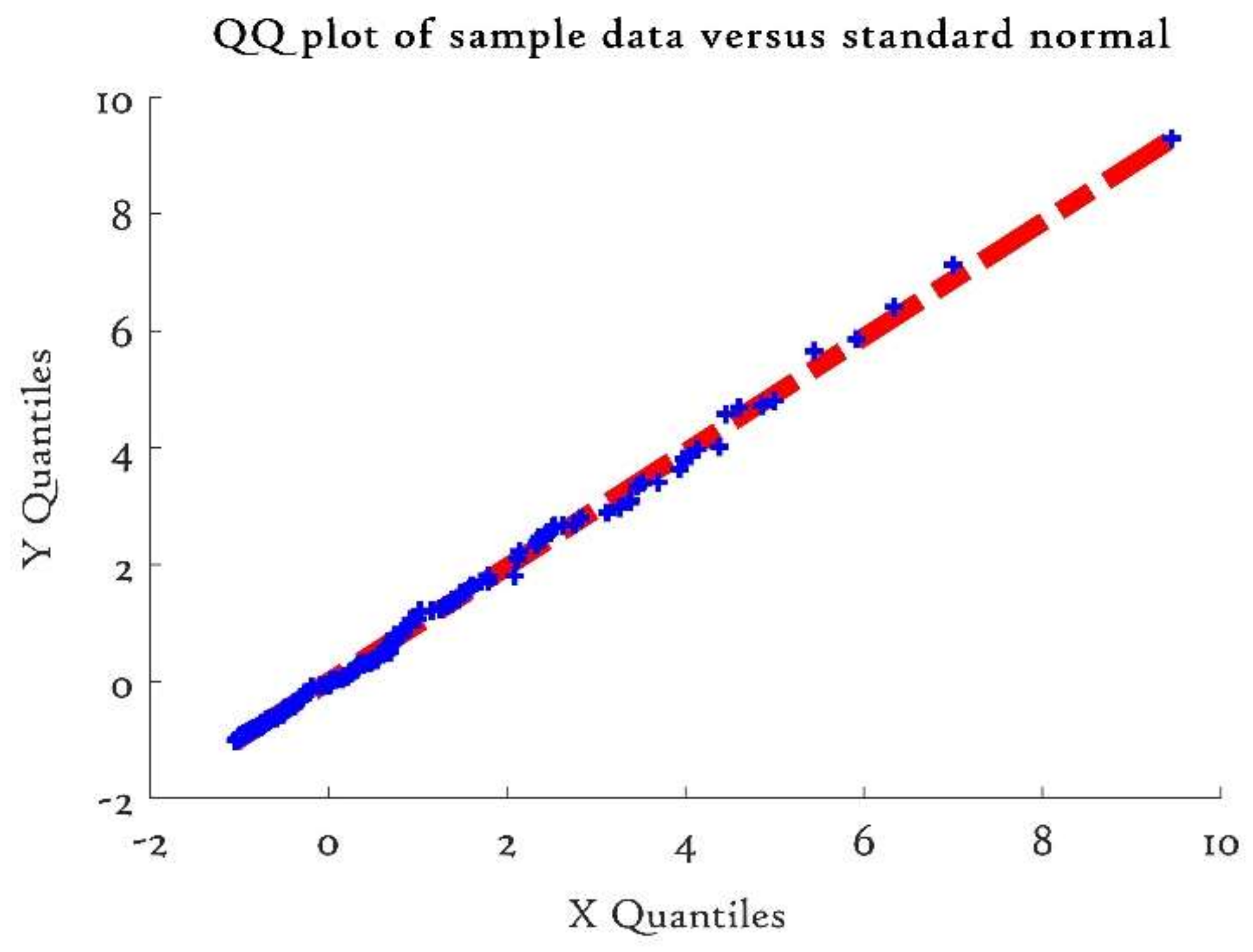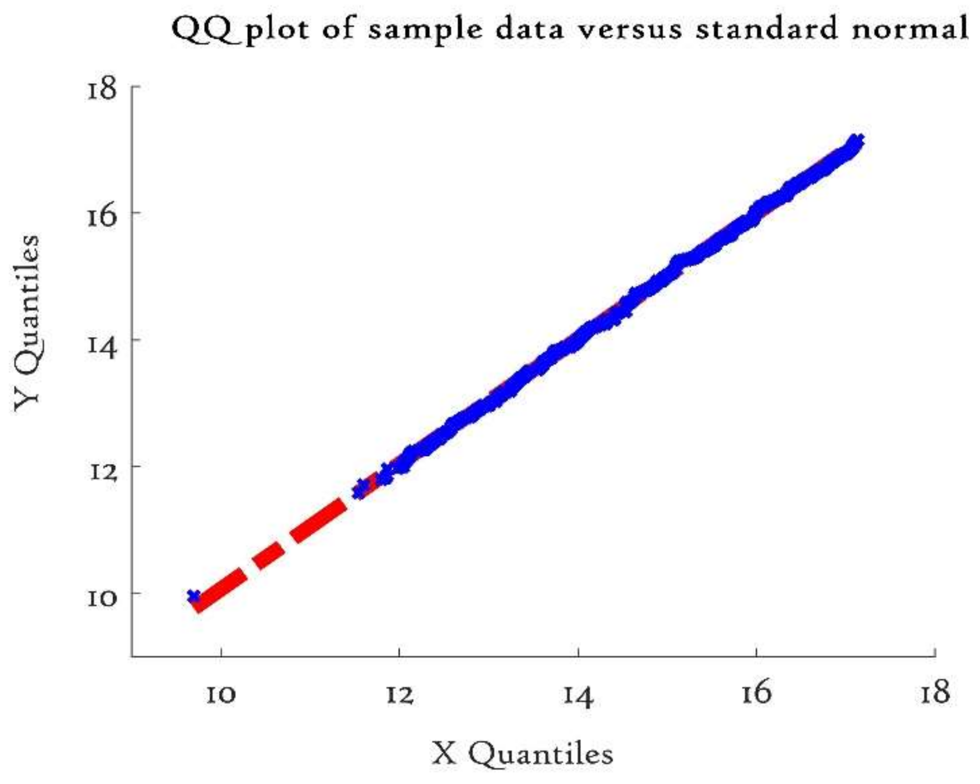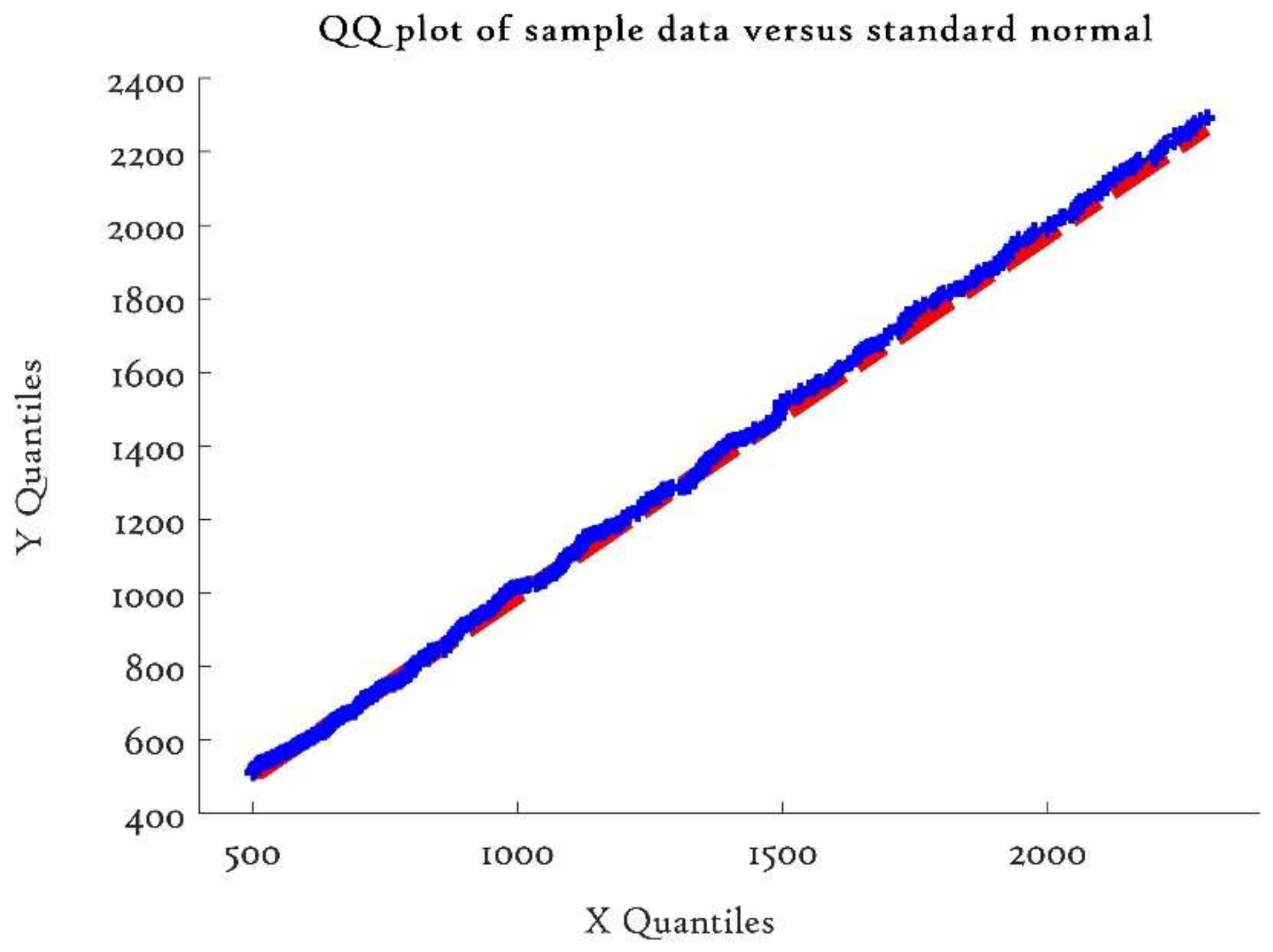Section 4 proposes a Gaussian Process model for building operational curves, including hyper-parameter optimization, and Section 5 presents the comparative analysis where uncertainty, residual distributions using the quantile-quantile (QQ) plot and error metrics analysis are used to evaluate the performance of GP operational curve models. Section 6 provides concluding remarks and future work.

2. Wind Turbine Operational Curves

Condition monitoring (CM) is a tool commonly employed for early detection of anomaly/failures to minimize downtime, maximize productivity and prevent catastrophic stage [3]. Incorporating critical variables (e.g., power, rotor speed, and blade pitch angle) to measure the impact of internal factors is an intelligent way to monitor the performance of the turbine. Continuous monitoring of these variables can be useful in identifying faults and enhanced wind turbine efficiency. Power curves, rotor curves, and blade pitch curves facilitated these variables and described as follows.

2.1. Power Curve

Wind farm operators widely use the Power Curve, considered as one of the fundamental data analysis practices. Accurate modeling of wind turbine power curves ensures precise performance monitoring and plays a significant role in forecasting the wind power generation [9]. The nonlinear relationship between power output and wind speed is depicted by a Power Curve of a Wind Turbine (Figure 1) and is useful in an energy assessment, warranty formulations, and performance monitoring of the turbines. The available active power is a function of wind speed distribution and the total available power in the wind, and its production highly depends on hub height wind speed and rated turbine efficiency and is mathematically expressed as [10],

$$P=0.5 \rho A{C}_p(\mathsf{\lambda },\beta )v^3$$

(1)

where $\rho$ is air density (kg/m₃), A is the swept area (${\mathrm{m}}^2$), $C_p$ is the power coefficient of the wind turbine and $v$ is the hub wind speed (m/sec).

The power coefficient depends on the tip speed ratio $(\lambda )$ and pitch angle $(\beta )$ and thus affects the power output of the wind turbine along with rotor speed. Moreover, the power performance of a wind turbine is highly influenced by other parameters associated with site conditions, for example, wind direction, wind shear, turbulence and others [9,17].

Air density affects the wind power production and hence the accuracy of the power curve and thus need particular attention. Air density is not constant, and it changes with wind farm site, altitude, and ambient temperature. The IEC 61400-12-1 [17] standards have guidelines for accurate power curve measurement of an individual wind turbine. The data used in this study were obtained from pitch regulated wind turbines, and as per the IEC standard [17]; air density correction should be applied using the following equations,

$$\mathsf{\rho }=1.225\left[\frac{288.15}{\mathrm{T}}\right]\left[\frac{\mathrm{B}}{1013.3}\right]$$

(2)

and,

$$V_C=V_M{\left[\frac{\rho }{1.225}\right]}^{\frac{1}{3}}$$

(3)

where $V_C$ and $V_M$ are the corrected and measured wind speed in m/sec, respectively, and the corrected air density is calculated by Equation (2) where B is atmospheric pressure in mbar and T the temperature in Kelvin. It is worth highlighting that the wind site farm parameters, e.g., location, altitude and ambient temperature, affect the air density. In Equation (3), B and T record 10-min average values obtained from SCADA datasets of an operational wind turbine. The calculated value of $\rho$ is then used in Equation (3) to calculate the corrected wind speed ($V_C$). This concept is used in the next section for developing correct and error free performance curves of a wind turbine.

2.2. Bade Pitch Curve

A blade pitch angle curve depicted the correlation between the turbine pitch angle and hub height wind speed and is shown in Figure 2. The pitch angle for three bladed wind turbines is calculated by averaging the angle of three blades. The pitch angle is adjusted by wind turbine operators to capture maximum power production and when the pitch angle is 90°, malfunction occurs due to high wind speed and causes a wind turbine to stall [33]. The presence of a strong wind signifies a negative value of the blade pitch angle and is widely used for power, performance and identifying malfunction of a wind turbine [33].

2.3. Rotor Curves

Rotor curves are broadly classified into two categories, to be specific; rotor speed curve and rotor power curve. The relationship between rotor speed and wind speed is the rotor speed curve and is shown in Figure 3 and is found after a cut in wind speed; rotor speed increases with wind speed. The rotor power curve that describes the relationship between rotor speed and power output of a wind turbine is illustrated in Figure 4. These curves are valuable in the investigation the malfunction caused by means of observing any difference from a typical rotor curve. For example, Singh [27] used a rotor curve to compare torque used for the rotor in comparison to the produced power, and if there is a difference between theoretical and calculated values, this needs to be investigated.

3. SCADA Data for Wind Turbine Performance Curves

These days, most wind farms are equipped with supervisory control and data acquisition (SCADA) systems that records the parameter which is broadly classified into controllable parameters (e.g., Blade pitch angle and generator torque), non-controllable parameters (e.g., wind speed, wind deviation) and performance parameters (e.g., power, generator speed, and gearbox speed). This recorded information contains continuous time observations such as load history and operation of the individual turbine, which can be utilized for overall turbine performance monitoring as well as play a significant role in identifying component failures without extra cost. The SCADA data used in this study are of 10 min (the industry standard) sampling interval and are taken from a robust wind turbine, located in Scotland, UK. In this study, monthly data from one wind turbine comprise more than 100 different signals, ranging from the timestamp, calculated values, set point, measurements of temperature, current, voltage, wind speed, power output, wind direction, etc., and are used for model training and validation purposes. For better understanding, SCADA data are generally divided into operational data, status data and warning data.

Sensor failures and data malfunction cause corrupt SCADA data and errors that make model analysis inaccurate and confusing and hence should not be used in the training stage. To obtain the best results, prior preprocessing of these data points is essential. Moreover, the GP model accuracy depends on the quality of data due to its nonparametric nature; the criteria are outlined in [41], for example, abnormal wind speed, timestamp mismatches, out of range values, negative power values, and turbine power curtailment is preformed to remove misleading data. Despite these adopted methodologies, SCADA data are not entirely free from error but minimize its impact significantly.

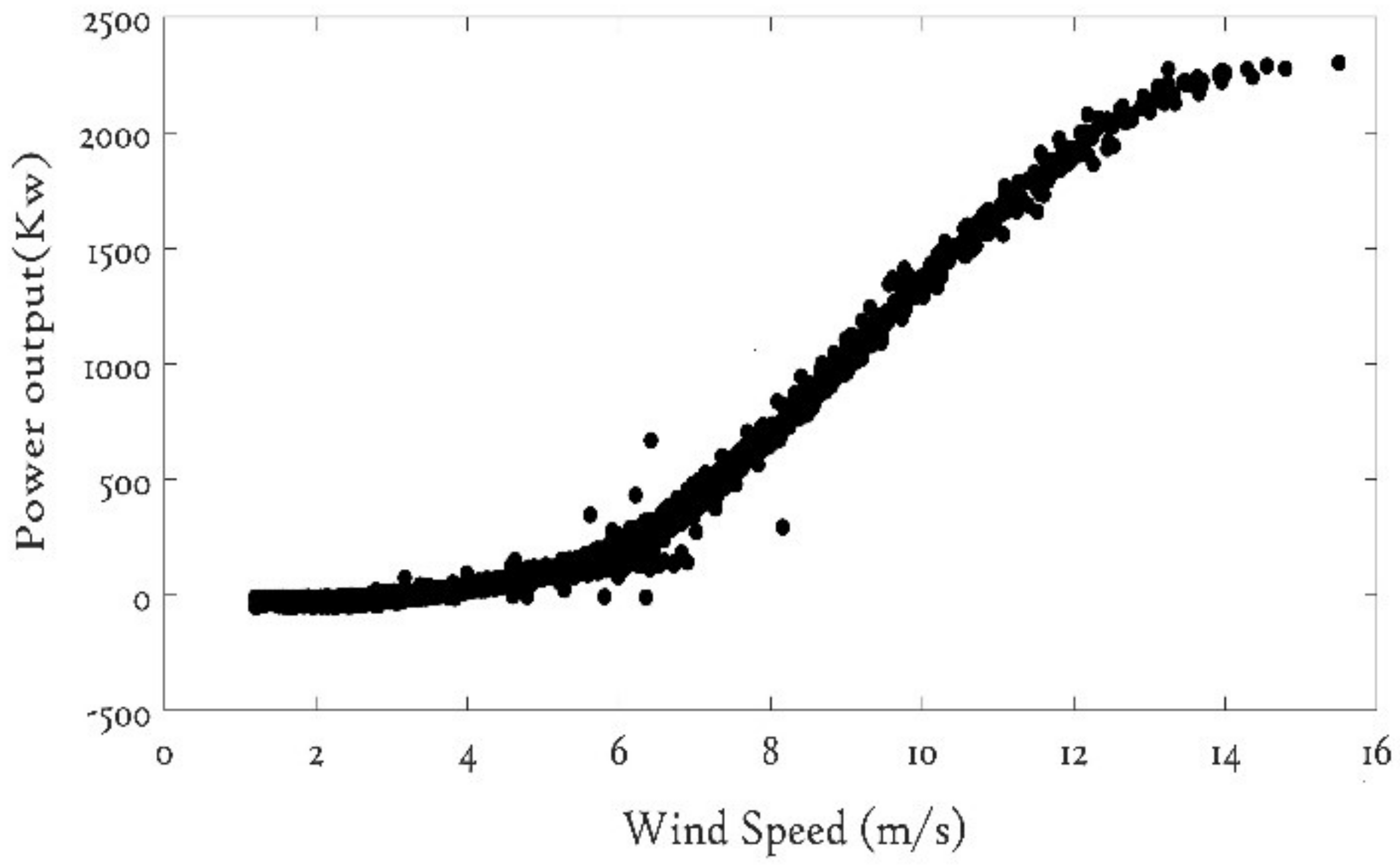
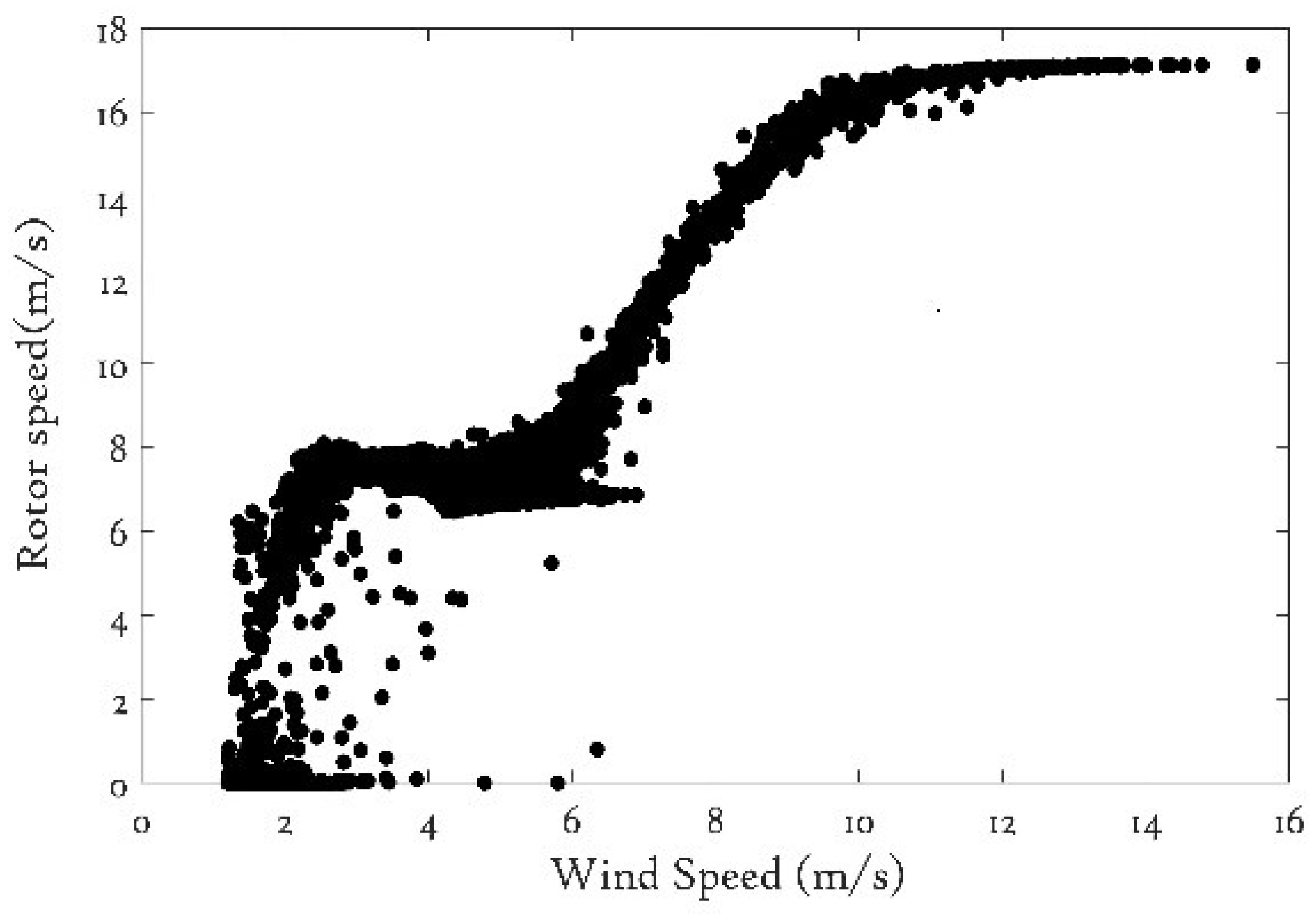
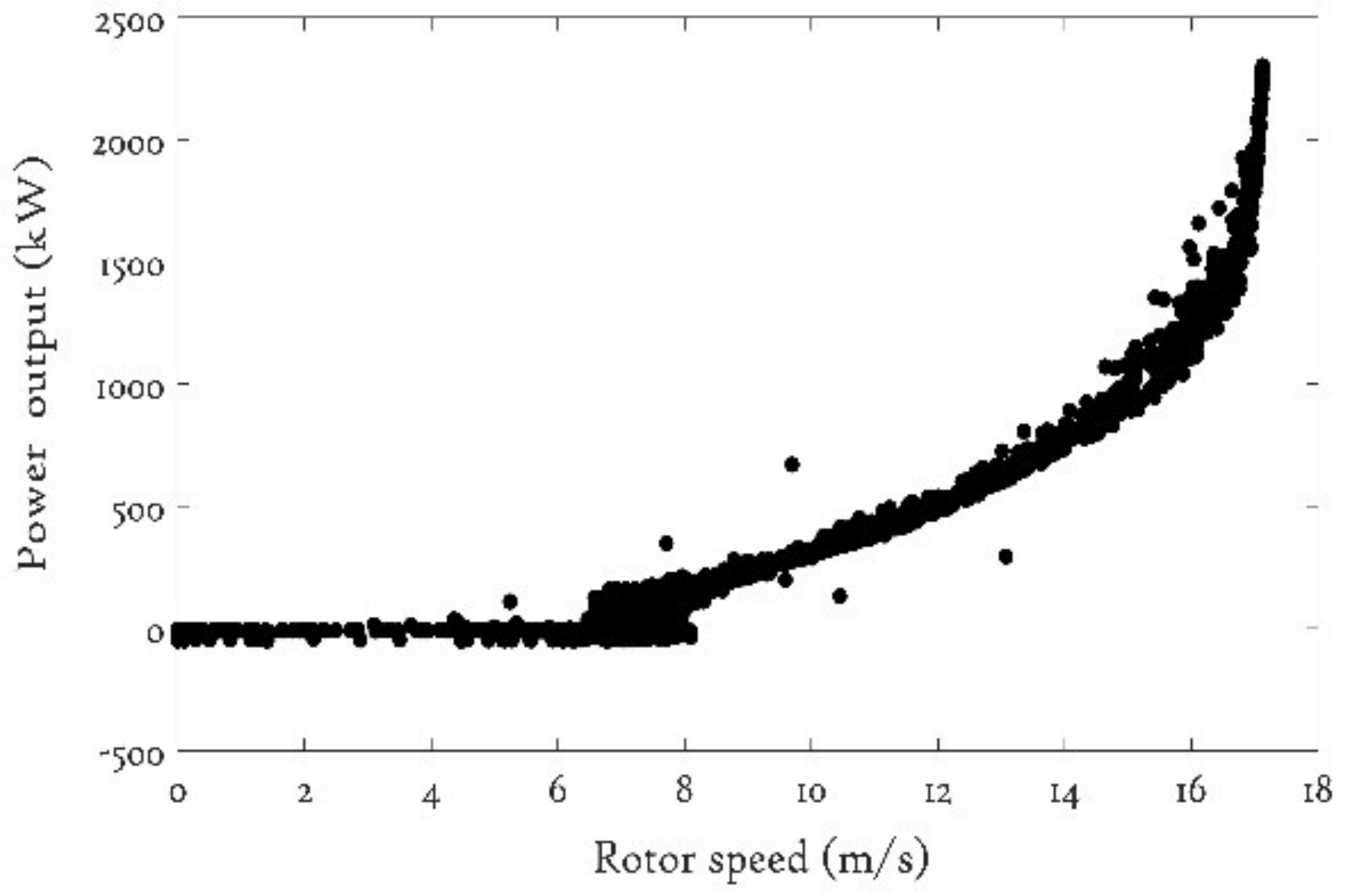
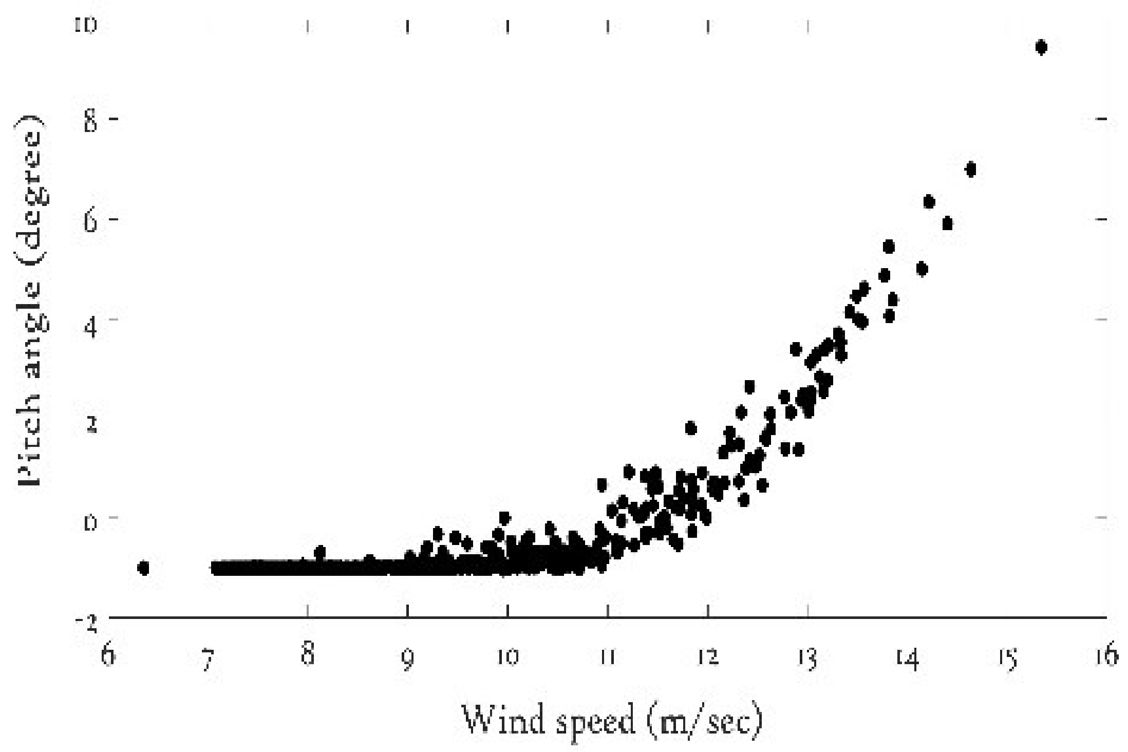
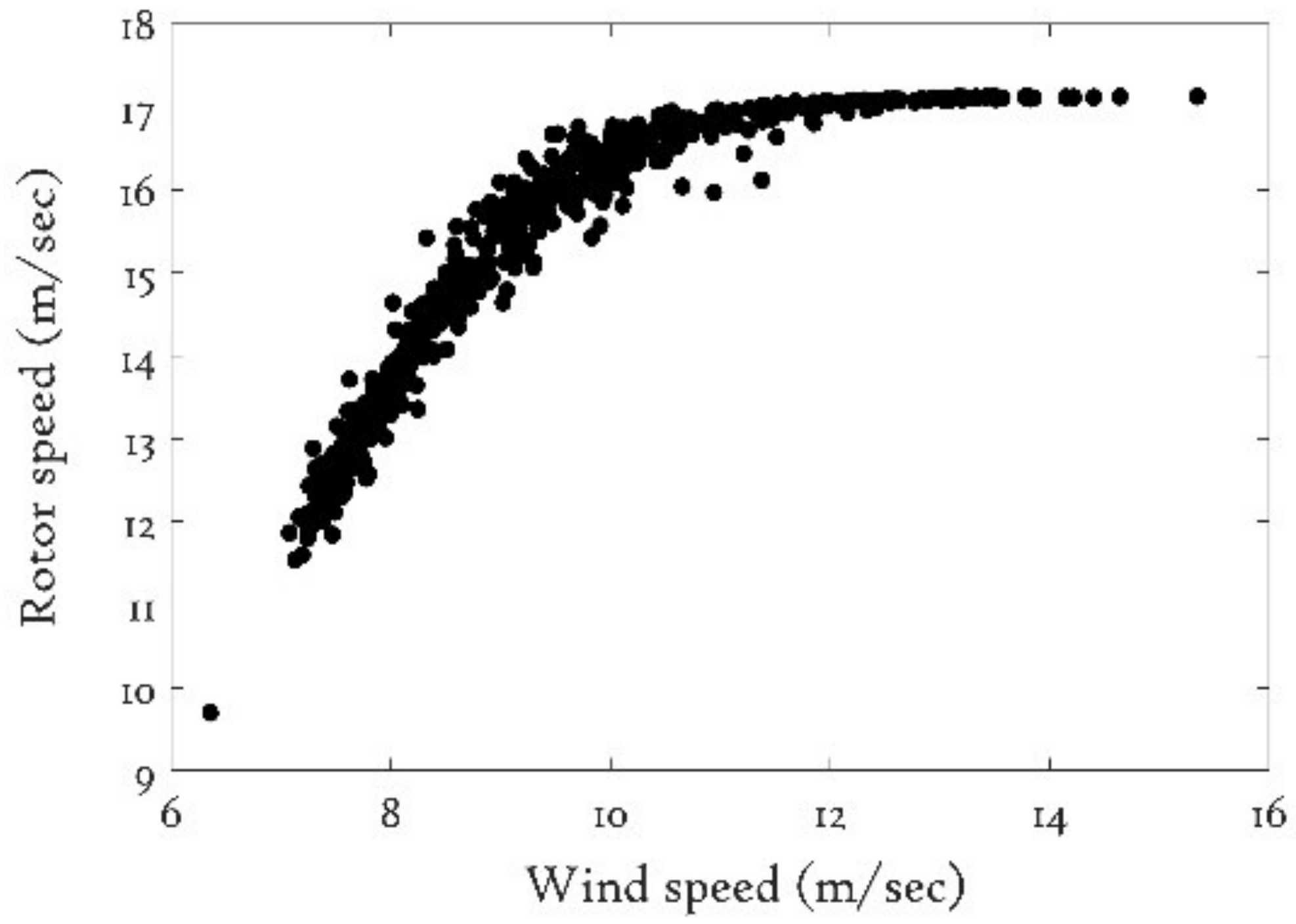
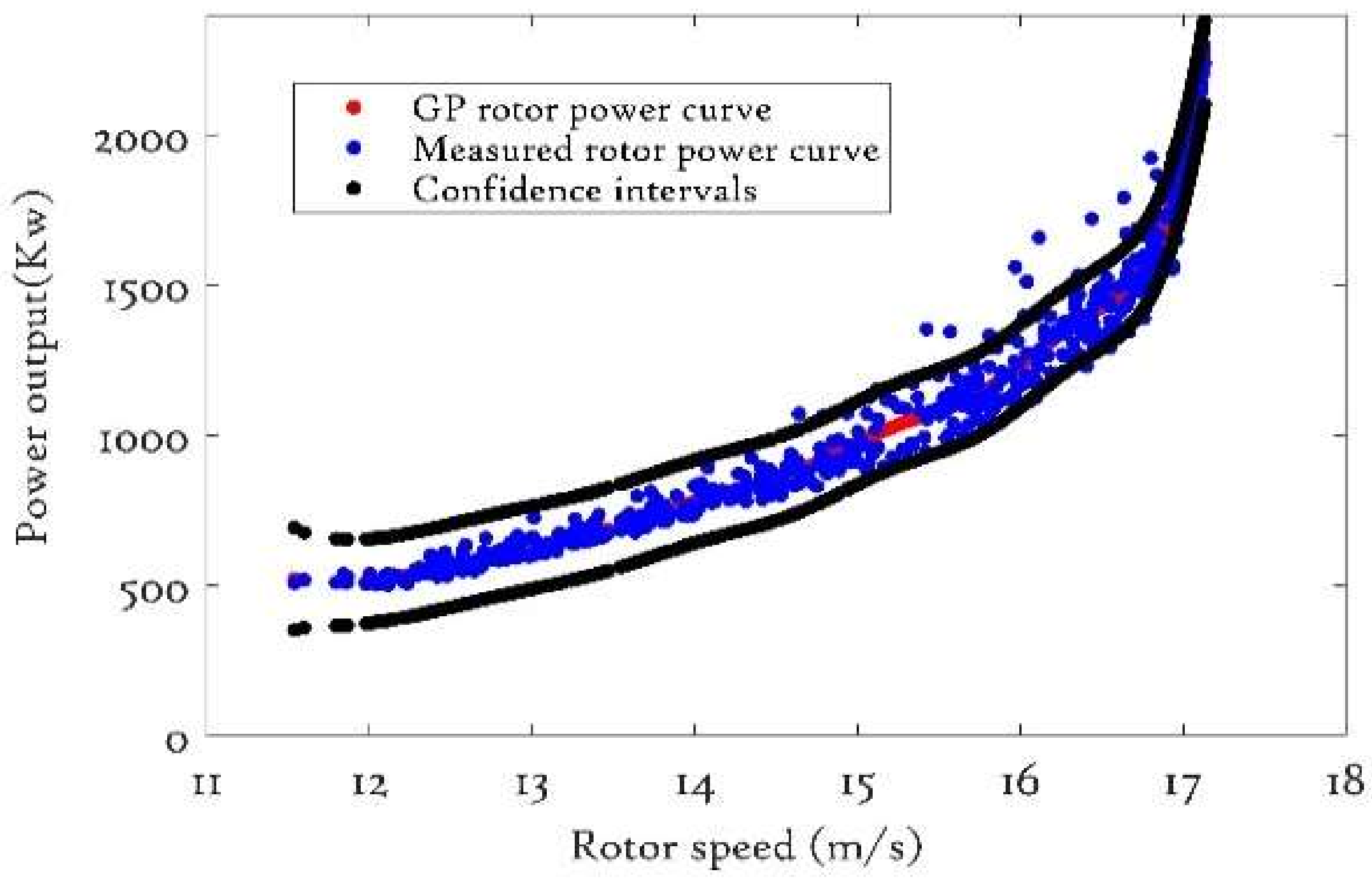
The data used in this study are from 2.3 MW Siemens turbines and contain 4464 data points that begin with the time stamp ‘‘1/7/2012 00:00 a.m.’’ and end at time stamp ‘‘31/7/2012 23:50 p.m.’’ The measured performance/operational curves using these data points are shown in Figure 1, Figure 2, Figure 3 and Figure 4. These measured data points became 626 data points after pre-processing (

Table 1. SCADA dataset description.

Start Timestamp	End Timestamp	Measured Data	Filtered Data
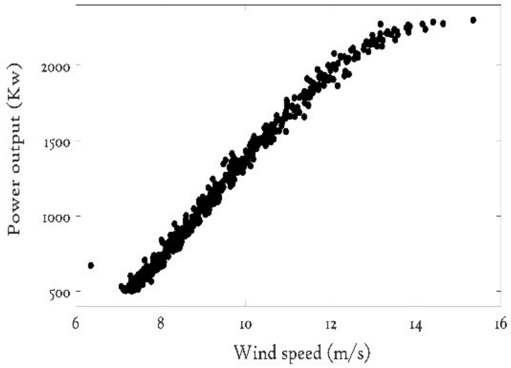
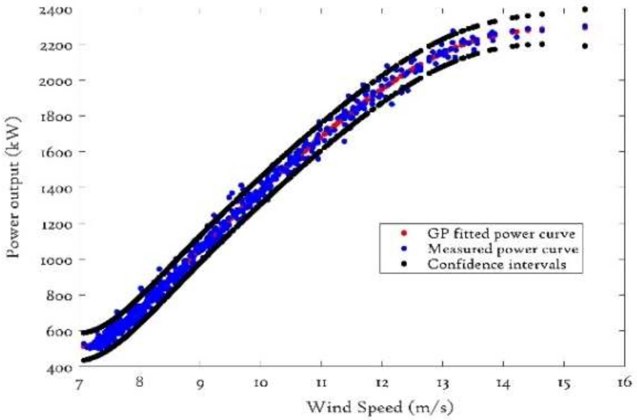
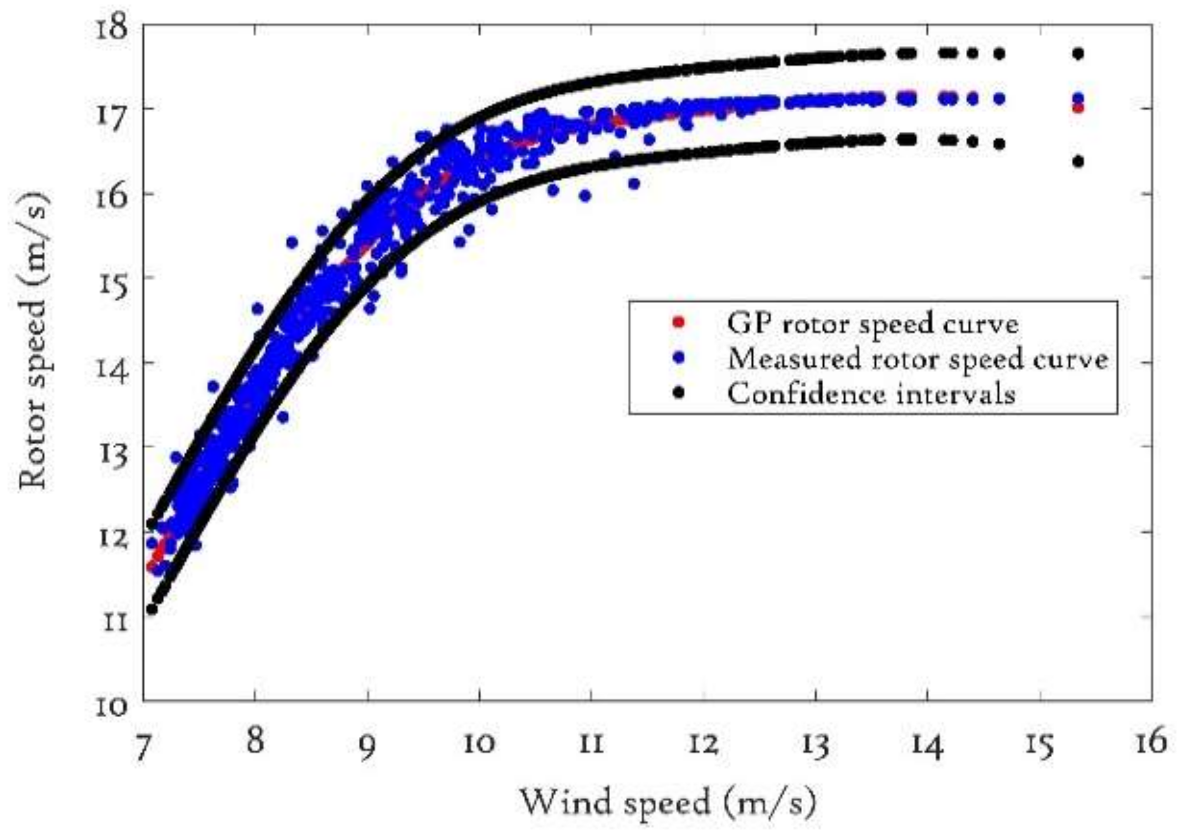
1/7/2012 00:00 a.m.	31/7/2012 23:50 p.m.	4464	626

) and were used to develop operational curves based on Gaussian Process models in upcoming sections. The preprocessed and air density corrected operational curves are shown in Figure 5, Figure 6, Figure 7 and Figure 8.

4. Operational Curve Modeling Using Gaussian Process

A Gaussian Process (GP) is a Bayesian, non-parametric, non-linear machine learning technique mainly used to deal with probabilistic regression and classification problems. In [35], a brief theory of GP is well presented and used in this study as follows.

Gaussian Processes (GPs) are the generalization of a Gaussian distribution over a finite vector space to a function space of infinite dimension [35]. A GP defines a prior over functions, which can be converted into a posterior over functions and intuitively, it can be thought of as defining a distribution over functions [42]. The inference of a GP takes place in the space of functions [35]. A GP, in essence, is the non-parametric generalization of a normal joint distribution for a given potentially infinite set of variables that gives an alternative way to solve nonlinear regression problems and because of its flexibility and ease of modeling, GP is considered ideal choice to solve complex issues associated with wind turbine condition monitoring. A GP is parameterized by a mean function $m(x)$ and covariance function $k(x,x^{\prime })$ and mathematically, for the location x, the GP f(x) expressed as by,

$$f(x)=GP(m(x),k(x,x^{\prime }))$$

(4)

where $k$ is the covariance function that has an associated probability density function:

$$P(x;m,k)=\frac{1}{{(2\mathsf{\pi })}^{\frac{n}{2}}{|\sum |}^{\frac{1}{2}}} \exp \left\{-\frac{1}{2}{(x-m)}^T k^{-1}(x-m)\right\}$$

(5)

where $|k|$ is defined as a determinant of $k$, $n$ is the dimension of random input vector $x$, and µ is mean vector of $x$. The term under the exponent, i.e., $\frac{1}{2}{(x-m)}^T k^{-1}(x-m)$ is an example of a quadratic shape, and the mean function is commonly fixed to zero [35].

The covariance functions or kernels measure the similarity between two data points to calculate the closeness and is the soul of any GP model. GP model behavior is entirely described by its co-variance functions which makes a selection of a suitable covariance function crucial for accurate GP modeling. A detailed presentation of many possible kernels is presented in [35,42], and selection is based on the nature of the data. In this study, squared exponential covariance function is used and for any finite collection of inputs $\{x1,x2,\dots ..,xn\}$, it is mathematically described as:

$$k_{SE} (x,x^{\prime })={\sigma }_f^2\exp (-\frac{{(x-x^{\prime })}^2}{2l^2})$$

(6)

As described already, SCADA data are not immune to measurement error, hence it is desirable to add a noise term to the covariance function to compensate the impact the measurement error and improve the accuracy of the GP model. Hence, Equation (6) can be altered to be:

$$k_{SE} (x,x^{\prime })={\sigma }_f^2\exp (-\frac{{(x-x^{\prime })}^2}{2l^2})+{\sigma }_n^2\delta (x,x\text{'})$$

(7)

where ${\sigma }_f^2$ and $l$ are known as the hyper-parameters. ${\sigma }_f^2$ signifies the signal variance and $l$ is a characteristic length scale which describes how quickly the covariance decreases with the distance between points. ${\mathsf{\sigma }}_n$ is the standard deviation of the noise fluctuation and gives information about model uncertainty. $\delta$ is the Kronecker delta [35].

The basic Gaussian Process regression (GPR) theory is inspired from [35] and is described as follows. The Gaussian Process regression model assumes that for a Gaussian process f observed at coordinates x, the vector of values $f(x)$ is just one sample from a multivariate Gaussian distribution of dimension equal to a number of measured coordinates $|x|$. Therefore, the $f(x)$ under zero-mean distribution function is

$$f(x)~\mathcal{N}(0,k(\theta ,x,x^{\prime }))$$

(8)

where $k(\theta ,x,x^{\prime })$ is the covariance matrix between all possible pairs $(x,x^{\prime })$ for a given set of hyper parameters $\theta$. The squared exponents have hyper parameters; ${\sigma }_f^2$, ${\sigma }_n^2$ and $l$ and need to be optimized for a better result. To do so, maximization of the log marginal likelihood described in [35] is used and is given below,

$$\begin{array}{c}log(p(f(x)|\theta ,x))=-0.5f{(x)}^{T}k{(\theta ,x,x^{\prime })}^{-1}f(x)-0.5log(|k(\theta ,x,x^{\prime })|)-\\ 0.5|x|log(2\pi )\end{array}$$

(9)

The maximization of this marginal likelihood towards θ provides the complete specification of the GP $f(x)$ and improves the model accuracy. Once hyperparameters have been optimized using Equation (9), the estimation of the distribution of $f(x)$ for a given $x^{\ast }$ is straightforward and taking the samples from the estimated distribution,

$$p(y^{\ast }|x^{\ast },f(x),x)=\mathcal{N}(y^{\ast }|A,B)$$

(10)

where A is the posterior mean estimate and is defined as,

$$A=k(\theta ,x^{\ast },x)k{(\theta ,x,x^{\prime })}^{-1}f(x)$$

(11)

Moreover, the posterior variance estimate B is defined as:

$$B=k(\theta ,x^{\ast },x^{\ast })-k(\theta ,x^{\ast },x)k{(\theta ,x,x^{\prime })}^{-1}k{(\theta ,x^{\ast },x)}^T$$

(12)

where $k(\theta ,x^{\ast },x)$ is the covariance between the new data points of estimation x* and all other measured coordinates x for a given hyper parameter vector θ, $k(\theta ,x,x^{\prime })$ and $f(x)$ are defined already and $k(\theta ,x^{\ast },x)$ is the variance at point x* as dominated by θ. It should be noted that that the posterior mean estimate $f(x^{\ast })$ is a linear combination of the observations $f(x)$; in a similar manner the variance of $f(x^{\ast })$ is actually independent of the observations $f(x^{\ast })$.

The covariance matrix, K, gives the variance of each variable along the leading diagonal, and the off-diagonal elements measure the correlations between the different variables mathematically described as follows:

$$K=\left[\begin{array}{ccc}{k}_{11}& \cdots & k_{1n}\\ ⋮& \ddots & ⋮\\ k_{n1}& \cdots & k_n\end{array}\right]\mathrm{where}{k}_{ij}=k(x_i,x_j)$$

$K$ is of size $n\times n$, where $n$ is the number of input parameters considered, and it must be symmetric and positive semidefinite, i.e., ${\sum }_{ij}={\sum }_{ji}$.

Using the filtered and corrected operational curve SCADA datasets (of Figure 5, Figure 6, Figure 7 and Figure 8), estimated operational curves were constructed using GP models (realized in MATLAB), and are shown in Figure 9, Figure 10, Figure 11 and Figure 12; GP closely following the expected variance. However, a large number of data points makes the GP model inaccurate due to its process involved in inverting a matrix of dimension computation of the marginal likelihood and is equal to the number of data points. This asymptotic complexity is called cubic inversion $O{(N)}^3$ where N is the number of data points. If N contains large data sets, then the computation of $N\times N$ matrix becomes problematic and affects the GP model accuracy. 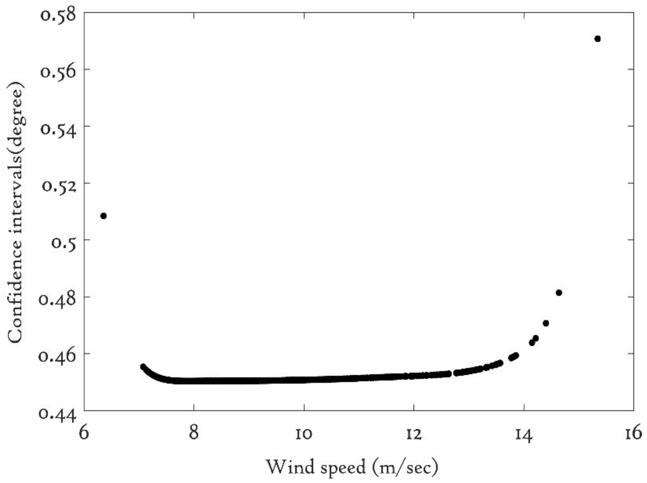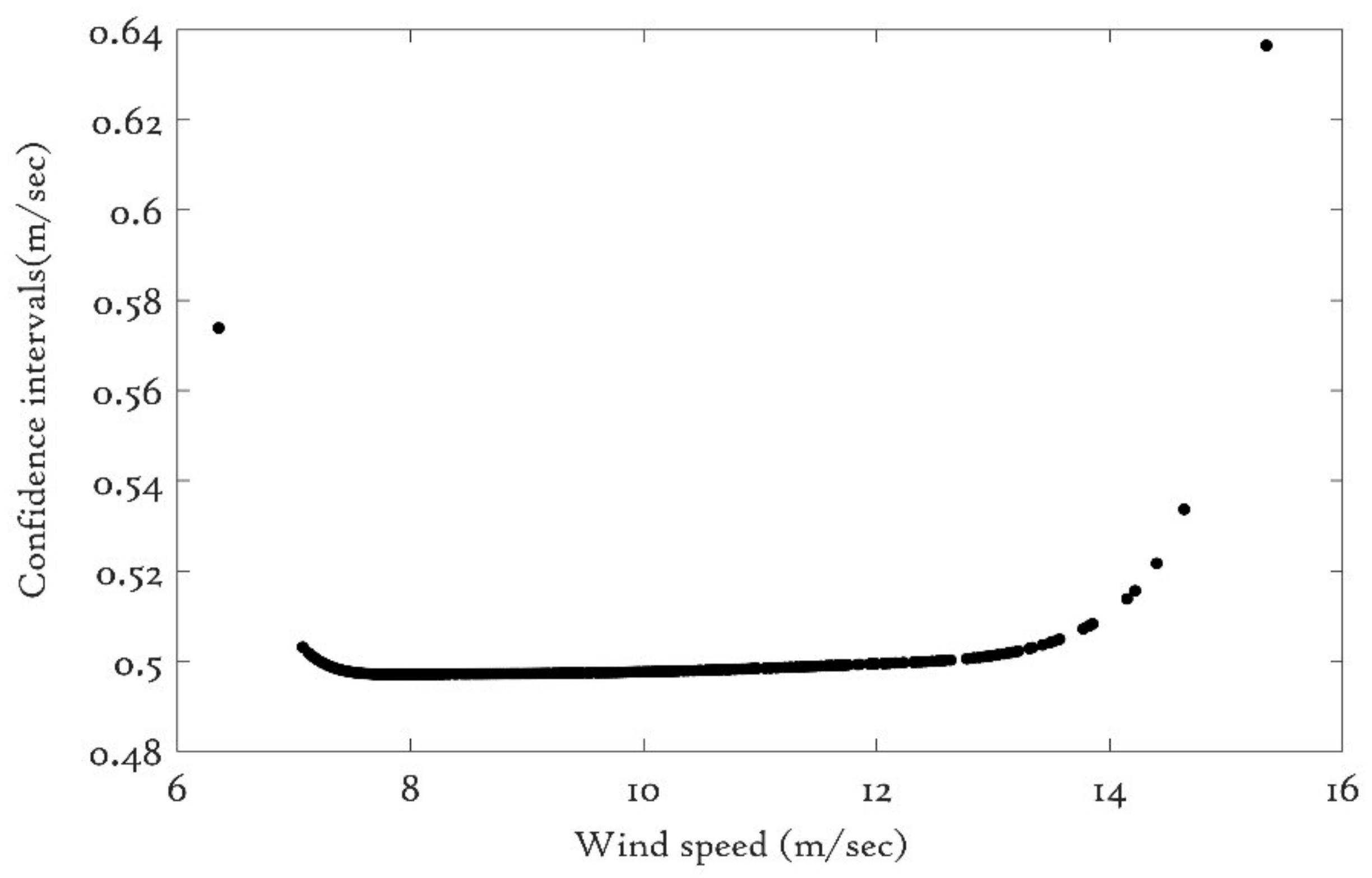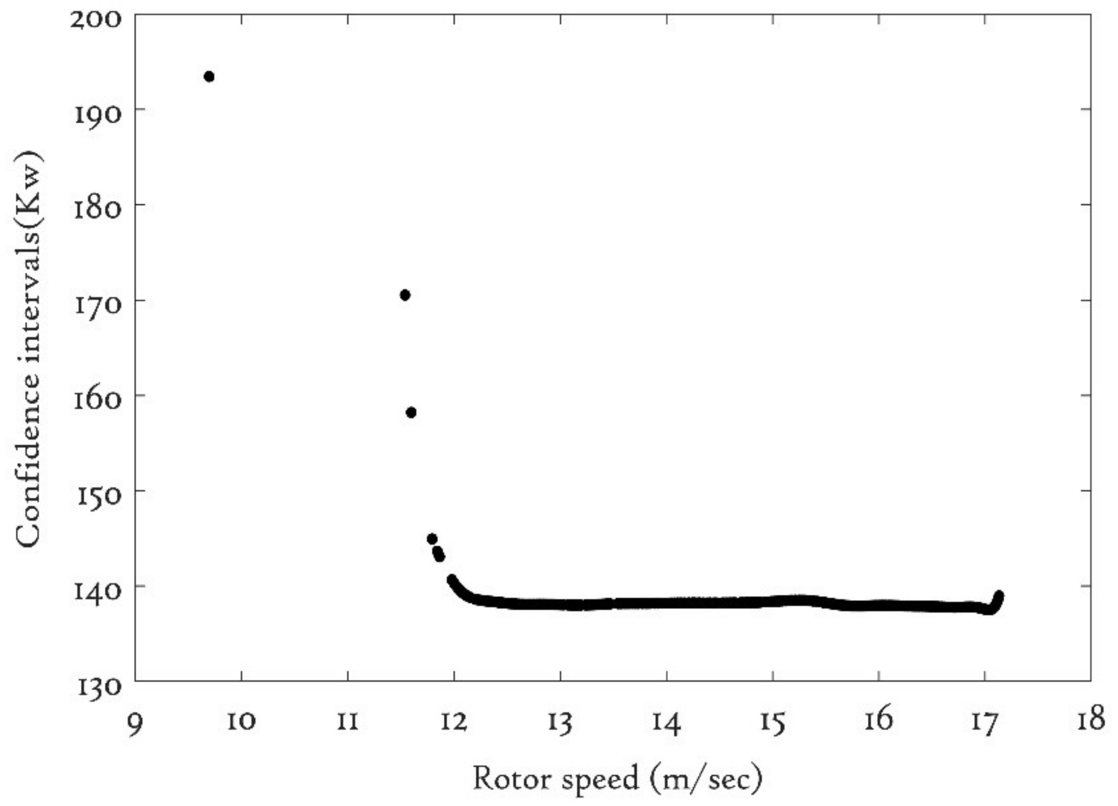Various techniques are proposed to solve this cubic inversion issues [43,44], yet these methods require high processing power and computational cost; however, GP works well with limited data sets. GP models have confidence intervals (CIs) that are valuable for uncertainty examination and are depicted in the next sections.

5. Comparative Analysis of Gaussian Process Operational Curves

In this section, we analyzed in detail the performance of the GP operational curves using the uncertainty analysis and residual distributions analysis, described as follows.

5.1. GP Operational Curve Uncertainty Analysis

SCADA systems have an unprecedented amount of data sets that lead to an urgent need for developing robust and accurate retrieval methods, which ideally should provide uncertainty intervals for the predictions. The uncertainty analysis is helpful for judging the performance of the models. GP models come with confidence intervals through Gaussian probability along with mean estimates which are a good indicator for evaluating the robustness and uncertainty model. The standard deviation is the square root of the variance of the predicted function $B$ (see Equation (12)) and is used to calculate the confidence intervals (chosen to be 95%) of the GP operational curves using Equation (13),

$$CIs=A\pm 2\surd B$$

(13)

In Equation (13), CIs represent the pointwise mean plus and minus two times the standard deviation for given input data (corresponding to the 95% confidence region which represents the significance level of 0.05), for the prior and posterior, respectively.

With the help of confidence intervals, unexpected data reflecting operational faults can be identified. It should be noted that confidence intervals give essential information about the uncertainty surrounding an estimation, but are themselves model-based estimates. In this study, operational curves with estimated 95% confidence intervals are used. The estimated operational curves with confidence intervals are shown in Figure 9, Figure 10, Figure 11 and Figure 12. Confidence intervals as a function of wind speed and rotor speed are plotted for estimating the accuracy of the GP operational curves and are shown in Figure 13, Figure 14, Figure 15 and Figure 16. The estimated GP power curve has less uncertainty as compared to GP rotor speed curve. Since GP is a form of data interpolation, data used in training and estimation impact the uncertainty. For example, the higher uncertainty in Figure 14 and Figure 15 reflects the fact that there are reduced numbers of data points in these areas.

5.2. Residual Distribution Analysis Using QQ Plots

The quantile-quantile or QQ plot is a simple graphical technique used to compare collections of data or theoretical distributions and is used to identify the distribution function. Identifying whether the distribution function is skewed or slightly tailed can be efficiently analyzed with the help of a QQ plot. A theoretical QQ plot examines whether or not a sample $S_1,$….., $S_n$ has come from a distribution with a given distribution function $F(s)$ and is plotted against the expected value for the specified distribution using sample of datasets starting from small to large values [45]. Compared to a histogram, the QQ plot is easy to interpolate. For example, Jean Dickinson [46], indicated that a QQ plot is easier to use than comparing histogram plots in order to judge skewness or more accurately assess whether the distribution tails are thicker or thinner than a normal distribution. Moreover, a QQ plot gives valuable information about graphical properties such as whether shape, location, size, and skewness are similar or different for two distributions and is thus used in this research.

As described above, QQ plots that compare two samples of data can be seen as a non-parametric approach to compare their underlying distributions and are hence used here for GP operational curve distribution analysis. Theoretically, residuals of a GP model should be Gaussian, and the typical QQ plot is a straight line with a unit gradient. QQ plots comparing the residual distribution with a Gaussian distribution for GP operational curves, see Figure 17, Figure 18, Figure 19 and Figure 20, suggest that estimated GP operational curves closely following a Gaussian distribution. QQ plot analysis is useful for identifying essential parameters such as skewnes, associated with GP operational curves. Thus, it is useful in wind turbine condition monitoring. Statistical performance indicators (RMSE and MAE) further validates this; see

Table 2. Statistical error for different GP models from QQ plots.

Sr.no	GP Operational Curves	RMSE	MAE
1	Power curve	2.223	1.423
2	Blade pitch curve	0.021	0.005
3	Rotor power curve	4.624	1.743
4	Rotor speed curve	0.011	0.004

(described in Section 5.3). The calculated values of RMSE and MAE suggest that GP-based rotor speed curve and blade pitch curve have a distribution function very close to the Gaussian distribution as compared to other GP operational curves.

5.3. GP Model Validations Using Error Metrics

Deterministic and probabilistic error metrics were used to evaluate the performance of GP operational curves. A brief review of the available error metrics can be found in [46]. In this study, root mean square (RMSE), mean absolute error (MAE) and coefficient of determination ($R^2$) were used and are described below.

The mean absolute error (MAE) is defined as the difference between the measured and estimated values and is suitable to describe the uniformly distributed errors. The MAE calculated the average error between the measured and the estimated values and is expressed as follows,

$$\mathrm{MAE}=\frac{{\sum }_{i=1}^{n}abs({A_i}^{\prime }-A_i)}{n}$$

(14)

The root mean square error (RMSE) is used to quantify the magnitude of residuals and is mathematically described as

$$\mathrm{RMSE}=\sqrt{\frac{{\sum }_{i=1}^n{(A_i^{\text{'}}-A_i)}^2}{n}}$$

(15)

where $A^{\prime }$ represents the Gaussian Process predicated values for $n$ different predictions, and $A$ represents the observed values. It is worth noting that using RMSE, the errors are unbiased and follow a normal distribution. The coefficient of determination ($R^2$), which signifies how close the data are to the fitted GP regression, is a widely used error matric to evaluate the performance of parametric and nonparametric models [46]. It is calculated as the square of the correlation between estimated output and measured values using: $R^2=1-\frac{SSE}{TSS}$ where SSE is the sum of squared errors and TSS is the total sum of squares. A higher value R² indicates a better coincidence of measured and estimated results. The calculated error metrics for GP operation curves are summarized in

Table 3. Statistical measures for GP operational curve models.

GP Operational Curves	RMSE	R2	MAE
Power curve	38.040	0.994	28.968
Pitch curve	0.228	0.965	0.107
Rotor speed curve	0.251	0.977	0.182
Rotor power curve	69.048	0.981	46.623

and suggest that GP accurately estimates the pattern of measured operational curves of a wind turbine. The RMSE and MAE calculated values suggest that among the operational curves, the GP blade pitch curve has a better prediction accuracy while $R^2$ suggests that the GP power curve distribution function is relatively better than that of other operational curves. Figure 21 is the time series comparison of GP operational curves.

6. Conclusions and Future Work

The relationship between critical parameters, for example, power, wind speed, blade angle and rotor speed can be used in early detection of faults and failures in order to improve the power performance of wind turbines. Gaussian Process models are a data-driven approach which is capable of formulating the relationship between these parameters due its multivariate property and therefore can be helpful in investigating the internal operation of wind turbines. In this paper, wind turbine operational curves using Gaussian Process (GP) models are presented which can be used to assess underperformance of wind turbines and thus improve their condition monitoring. The critical performance variables of turbines are used to develop GP operational curves, and these are power, wind speed, blade pitch angle and rotor speed. GP operational curves (power curve, rotor curve and blade pitch curve) are practical tools to study and visualize the behavior of wind turbines during operational conditions. The statistical performance metrics (Table 3) suggest that GP models are able to estimate the operational curves accurately while QQ plot analysis concludes that GP operational curves distribution functions are close to the Gaussian distribution. The calculated confidence intervals of GP operational curves measure the model uncertainty and can play a significant role in constructing fault detection algorithms. A SCADA dataset was obtained from a robust wind turbine and has been used to model the GP operational curves.

Future work will use GP operational curves to identify the major failures of wind turbines.

References

1. Wind Energy in the UK State of the Industry Report. 2015. Available online: http://c.ymcdn.com/sites/www.renewableuk.com/resource/resmgr/publications/reports/soi_report_summary_2015.pdf (accessed on 5 May 2018).
2. Sheng, S. Prognostics and Health Management of Wind Turbines: Current Status and Future Opportunities; NREL/PR-5000–65605; National Renewable Energy Laboratory: Golden, CT, USA, 2015.
3. Yang, W.X.; Tavner, P.J.; Crabtree, C.J.; Wilkinson, M. Cost effective condition monitoring for wind turbines. IEE Trans. Ind. Electron. 2009, 57, 263–271. [Google Scholar] [CrossRef] [Green Version]
4. Marquez, F.P.G. An Approach to Remote Condition Monitoring Systems Management. In Proceedings of the IET International Conference on Railway Condition Monitoring, Birmingham, UK, 29–30 November 2006; pp. 156–160. [Google Scholar]
5. Marquez, F.P.G.; Roberts, C.; Tobias, A. Railway point mechanisms: Condition monitoring and fault detection. Proceed. Inst. Mech. Eng. Part F J. Rail Rapid Transit 2010, 224, 35–44. [Google Scholar] [CrossRef]
6. Dao, P.; Staszewski, W.; Barszce, T.; Uhl, T. Condition monitoring and fault detection in wind turbines based on cointegration analysis of SCADA data. Renew. Energy 2018, 116, 107–122. [Google Scholar] [CrossRef]
7. Sun, P.; Li, J.; Wang, C.; Lei, X. A generalized model for wind turbine anomaly identification based on SCADA data. Appl. Energy 2016, 168, 550–567. [Google Scholar] [CrossRef] [Green Version]
8. Wang, Y.; Ma, H.; Wang, D.; Wang, G.; Wu, J.; Bian, J.; Liu, J. A new method for wind speed forecasting based on copula theory. Environ. Res. 2018, 160, 365–371. [Google Scholar] [CrossRef] [PubMed]
9. Ouyanga, T.; Kusiak, A.; Heb, Y. Modeling wind-turbine power curve: A data partitioning and mining approach. Renew. Energy 2017, 102, 1–8. [Google Scholar] [CrossRef]
10. Taslimi-Renani, E.; Modiri-Delshad, M.; Elias, M.F.M.; Rahim, N.A. Development of an enhanced parametric model for wind turbine power Curve. Appl. Energy 2016, 177, 544–552. [Google Scholar] [CrossRef]
11. Panahi, D.; Deilami, S.; Masoum, M.A.S. Evaluation of Parametric and Non-Parametric Methods for Power Curve Modelling of Wind Turbines. In Proceedings of the 9th International Conference on Electrical and Electronics Engineering (ELECO), Bursa, Turkey, 26–28 November 2015; pp. 996–1000. [Google Scholar]
12. Pelletier, F.; Masson, C.; Tahan, A. Wind turbine power curve modelling using artificial neural network. Renew. Energy 2016, 89, 207–214. [Google Scholar] [CrossRef]
13. Jurgen, H.; Mohammad, R.; Martin, B.; Niels, P.; Esmaeil, N. Bayesian state prediction of wind turbine bearing failure. Renew. Energy 2018, 116, 164–172. [Google Scholar]
14. Van der Meer, D.W.; Shepero, M.; Svensson, A.; Widén, J.; Munkhammar, J. Probabilistic forecasting of electricity consumption, photovoltaic power generation and net demand of an individual building using Gaussian Processes. Appl. Energy 2018, 213, 195–207. [Google Scholar] [CrossRef]
15. Lydia, M.; Kumar, S.S.; Selvakumar, A.I.; Prem Kumar, G.E. A comprehensive review on wind turbine power curve modeling techniques. Renew. Sustain. Energy Rev. 2014, 30, 452–460. [Google Scholar] [CrossRef]
16. Burton, T.; Jenkins, N.; Sharpe, D.; Bossanyi, E. Wind Energy Handbook, 2nd ed.; John Wiley & Sons: Chichester, UK, 2001. [Google Scholar]
17. International Standard IEC61400-12-1. Wind Turbines—Part 12-1: Power Performance Measurements of Electricity Producing Wind Turbines; IEC 61400-12-1; British Standard: London, UK, 2006. [Google Scholar]
18. Pandit, R.K.; Infield, D. Comparison of binned and Gaussian Process based wind turbine power curve for condition monitoring purposes. J. Maint. Eng. 2017, 2, 314–325. [Google Scholar]
19. Gill, S.; Stephen, B.; Galloway, S. Wind turbine condition assessment through power curve copula modeling. IEEE Trans. Sustain. Energy 2012, 3, 94–101. [Google Scholar] [CrossRef]
20. Thapar, V.; Agnihotri, G.; Sethi, V.K. Critical analysis of methods for mathematical modelling of wind turbines. Renew. Energy 2011, 36, 3166–3177. [Google Scholar] [CrossRef]
21. Wind Power in the United States: Technology, Economic, and Policy Issues. Available online: http://www.fas.org/sgp/crs/misc/RL34546.pdf (accessed on 5 April 2018).
22. Wiratama, I.K.; Nuarsa, I.M. Investigation of factors affecting power curve wind turbine blade. ARPN J Eng. Appl. Sci. 2016, 11, 5. [Google Scholar]
23. Sudhamshu, A.R.; Pandey, M.C.; Sunil, N.; Satish, N.S.; Mugundhan, V.; Velamati, R.K. Numerical study of effect of pitch angle on performance characteristics of a HAWT. Eng. Sci. Technol. Int. J. 2016, 19, 632–641. [Google Scholar]
24. Oueslati, M.M.; Dahmouni, A.W.; Nasrallah, S.B. Effects of sudden change in pitch angle on oscillating wind turbine airfoil performances. Eng. Anal. Bound. Elem. 2017, 81, 21–34. [Google Scholar] [CrossRef]
25. Zhang, J.; Cheng, M.; Chen, Z.; Fu, X. Pitch Angle Control for Variable Speed Wind Turbines. In Proceedings of the Third International Conference on Electric Utility Deregulation and Restructuring and Power Technologies, Nanjing, China, 6–9 April 2008; pp. 2691–2696. [Google Scholar]
26. Li, C.; Xiao, Y.; Xu, Y.; Peng, Y.; Hu, G.; Zhu, S. Optimization of blade pitch in H-rotor vertical axis wind turbines through computational fluid dynamics simulations. Appl. Energy 2018, 212, 1107–1125. [Google Scholar] [CrossRef]
27. Singh, P. Analytical Techniques of SCADA Data to Assess Operational Wind Turbine Performance. Master’s Thesis, University of Strathclyde, Glasgow, UK, 2013. [Google Scholar]
28. Kusiak, A.; Verma, A. A Data-Driven Approach for Monitoring Blade Pitch Faults in Wind Turbines. IEEE Trans. Sustain. Energy 2011, 2, 87–96. [Google Scholar] [CrossRef]
29. Wang, Z.; Zhuang, M. Leading-edge serrations for performance improvement on a vertical-axis wind turbine at low tip-speed-ratios. Appl. Energy 2017, 208, 1184–1197. [Google Scholar] [CrossRef]
30. Chen, W.; Chen, C.; Huang, C.; Hwang, C. Power output analysis and optimization of two straight-bladed vertical-axis wind turbines. Appl. Energy 2017, 185, 223–232. [Google Scholar] [CrossRef]
31. Rezaeiha, A.; Kalkman, I.; Blocken, B. Effect of pitch angle on power performance and aerodynamics of a vertical axis wind turbine. Appl. Energy 2017, 197, 132–150. [Google Scholar] [CrossRef]
32. Ma, N.; Lei, H.; Han, Z.; Zhou, D.; Bao, Y.; Zhang, K.; Zhou, L.; Chen, C. Airfoil optimization to improve power performance of a high-solidity vertical axis wind turbine at a moderate tip speed ratio. Energy 2018, 150, 236–252. [Google Scholar] [CrossRef]
33. Kusiak, A.; Verma, A. Monitoring Wind Farms with Performance Curves. IEEE Trans. Sustain. Energy 2013, 4, 192–199. [Google Scholar] [CrossRef]
34. Li, H.; Shi, K.L.; McLaren, P.G. Neural network based sensorless maximum wind energy capture with compensated power coefficient. IEEE Trans. Ind. Appl. 2005, 41, 1548–1556. [Google Scholar] [CrossRef]
35. Rasmussen, C.E.; Williams, C.K.I. Gaussian Processes for Machine Learning; The MIT Press: London, UK, 2006; ISBN 026218253X. [Google Scholar]
36. Yan, J.; Li, K.; Bai, E.W. Prediction Error Adjusted Gaussian Process for Short-Term Wind Power Forecasting. In Proceedings of the 2013 IEEE International Workshop on Intelligent Energy Systems (IWIES), Vienna, Austria, 14 November 2013; pp. 173–178. [Google Scholar]
37. Sheng, H.; Member, S.; Xiao, J.; Cheng, Y.; Member, S.; Ni, Q. Short-term solar power forecasting based on weighted Gaussian process regression. IEEE Trans. Ind. Electron. 2018, 65, 1–10. [Google Scholar] [CrossRef]
38. Mori, H.; Nakano, K. Development of Advanced Gaussian Process for LMP Forecasting. In Proceedings of the 18th International Conference on Intelligent System Application to Power Systems (ISAP), Porto, Portugal, 11–16 September 2015; pp. 1–6. [Google Scholar]
39. Papatheou, E.; Dervilis, N.; Maguire, A.E.; Campos, C.; Antoniadou, I.; Worden, K. Performance monitoring of a wind turbine using extreme function theory. Renew Energy 2017, 113, 1490–1502. [Google Scholar] [CrossRef]
40. Park, J.; Kwon, S.-D.; Law, K.H. A Data-Driven Approach for Cooperative Wind Farm Control. In Proceedings of the American Control Conference (ACC), Boston, MA, USA, 6–8 July 2016; pp. 525–530. [Google Scholar]
41. Schlechtingen, M.; Santos, I.F. Comparative analysis of neural network and regression based condition monitoring approaches for wind turbine fault detection. Mech. Syst. Signal Process. 2011, 25, 1849–1875. [Google Scholar] [CrossRef] [Green Version]
42. Murphy, K.P. Machine Learning: A Probabilistic Perspective, 1st ed.; Adaptive Computation and Machine Learning Series; The MIT Press: London, UK, 2018. [Google Scholar]
43. Hartikainen, J.; Särkkä, S. Kalman Filtering and Smoothing Solutions to Temporal Gaussian Process Regression Models. In Proceedings of the IEEE International Workshop on Machine Learning for Signal Processing, Kittila, Finland, 29 August–1 September 2010; pp. 379–384. [Google Scholar]
44. Sarkka, S.; Solin, A.; Hartikainen, J. Spatiotemporal learning via infinite-dimensional Bayesian filtering and smoothing. IEEE Signal Process. Mag. 2013, 30, 51–61. [Google Scholar] [CrossRef]
45. Wilk, M.B.; Gnanadesikan, R. Probability Plotting Methods for the Analysis of Data. Biometrika 1968, 55, 1–17. [Google Scholar] [CrossRef] [PubMed]
46. Gibbons, J.D.; Chakraborti, S. Nonparametric Statistical Inference, 4th ed.; Revised and Expanded; CRC Press: Boca Raton, FL, USA, 2014. [Google Scholar]
Figure 1. Measured Power Curve.
Energies 11 01631 g001
Figure 2. Measured Pitch angle curve.
Energies 11 01631 g002
Figure 3. Measured Rotor speed curve.
Energies 11 01631 g003
Figure 4. Measured rotor power curve.
Energies 11 01631 g004
Figure 5. Filtered power curve.
Energies 11 01631 g005
Figure 6. Filtered blade pitch curve.
Energies 11 01631 g006
Figure 7. Filtered rotor speed curve.
Energies 11 01631 g007
Figure 8. Filtered rotor power curve.
Energies 11 01631 g008
Figure 9. GP power curve with CIs.
Energies 11 01631 g009
Figure 10. GP blade pitch curve with CIs.
Energies 11 01631 g010
Figure 11. GP rotor speed curve with CIs.
Energies 11 01631 g011
Figure 12. GP rotor power curve with CIs.
Energies 11 01631 g012
Figure 13. GP power curve uncertainty.
Energies 11 01631 g013
Figure 14. GP blade curve uncertainty.
Energies 11 01631 g014
Figure 15. GP rotor speed curve uncertainty.
Energies 11 01631 g015
Figure 16. GP rotor power curve uncertainty.
Energies 11 01631 g016
Figure 17. QQ plot for GP power curve.
Energies 11 01631 g017
Figure 18. QQ plot for GP blade pitch curve.
Energies 11 01631 g018
Figure 19. QQ plot for GP rotor speed curve.
Energies 11 01631 g019
Figure 20. QQ plot for GP rotor power curve.
Energies 11 01631 g020
Figure 21. Comparative studies of measured and estimated operational curves in time series.
Energies 11 01631 g021