Abstract
Along with the high growth rate of economy and fast increasing air pollution, clean energy, such as the natural gas, has played an important role in preventing the environment from discharge of greenhouse gases and harmful substances in China. It is very important to accurately forecast the demand of natural gas in China is for the government to formulate energy policies. This paper firstly proposes a combined forecasting model, name GM-S-SIGM-GA model, to forecast the demand of natural gas in China from 2011 to 2017, by constructing the grey model (GM(1,1)) and the self-adapting intelligent grey model (SIGM), respectively; then, it employs a genetic algorithm to determine the combined weight coefficients between these two models. Finally, using the tendency index (the annual changes of the share of natural gas consumption from the total energy consumption), which completely reveal the annual natural gas consumption share among the market, to successfully adjust the fluctuated changes for each data period. The natural gas demand data from 2002 to 2010 in China are used to model the proposed GM-S-SIGM-GA model, and the data from 2011 to 2017 are used to evaluate the forecasting accuracy. The experimental results demonstrate that the proposed GM-S-SIGM-GA model is superior to other single forecasting models in terms of the mean absolute percentage error (MAPE; 4.48%), the root mean square error (RMSE; 11.59), and the mean absolute error (MAE; 8.41), respectively, and the forecasting performances also receive the statistical significance under 97.5% and 95% confident levels, respectively.
1. Introduction
1.1. Motivation
Along with the high growth rate of economy and fast increasing air pollution, clean energy such as natural gas has played an important role to prevent the environment from discharge of greenhouse gases and harmful substances. Natural gas is well known as a clean (burns cleaner), cheap (with high heating power than other fossil fuel), and low-carbon fossil fuel, it is the most realistic option for clean energy supply [1]. Particularly, as shown in the 13th Five-Year Plan of China, the development of natural gas industry has been an important national policy, in addition, due to environmental management and rapid increase in natural gas consumption that cause the imbalance between supply and demand [2]. On the other hand, the electricity utility companies are also motived to receive accurate natural gas consumption for their integrated demand response program switching the energy resources (from the electricity to the natural gas) during the peak hours [3,4]. Electricity utility companies should collaborate together to achieve sustainability in terms of providing more realistic forecasting models of interdependent natural gas demand networks [5]. Therefore, it is very important to accurately forecast the demand of natural gas in China for the government and energy companies to formulate energy policies.
1.2. Relevant Literature Reviews
Natural gas demand is not only related to population, energy consumption, and industrial and economic development, but also related to national energy policy, which have increased the complexity of natural gas demand forecasting work. In the past few decades, many natural gas demand forecasting models have been proposed to forecast natural gas consumption. These forecasting models can be classified into three main classes [6]: statistical models, intelligent models, and grey forecasting models. The other one is applications of artificial intelligent technology. The statistical models use historical data to find out the relationships among several time periods or variables, which contains the autoregressive integrated moving average (ARIMA) models [7,8], regression models [9,10,11], logistic based models [12,13], and Bayesian estimation models [14,15]. However, due to theoretical definitions, these statistical models could only deal well with linear relationships among natural gas demand and relevant factors. In addition, these models require sufficient historical data to determine suitable their parameters. Therefore, these models could only receive unsatisfied forecasting performance [6].
With powerful nonlinear reliance capability, the intelligent models have been employed to receive higher performances in natural gas demand forecasting, such as artificial neural networks (ANNs) [16,17,18,19], hybrid intelligent (evolutionary/heuristic algorithm, wavelet transform, and fuzzy theory) models [20,21,22,23], and support vector regression models [24,25,26,27]. Similarly, these intelligent models require very large amounts of data for training to determine well their embedded parameters to obtain satisfied forecasting accuracy [28]. Therefore, to overcome the drawbacks of these models, hybridizing or combining these models with each other to construct new or novel forecasting models has become the research hot point in the recent years, for example, hybridizing or combining with each other [17,18,21,22,27], and with evolutionary algorithms [20,21,25]. However, these intelligent models still have the theoretical shortcomings, such as time consumption, embedded parameters determination, and premature problems. Therefore, it is a feasible improvement to assign different weights according to different forecasting models.
On the other hand, proposed by Deng [29] in 1982, the grey forecasting model is superior to deal with small data set and poor information [6], and has been widely applied in many forecasting research fields. In addition, as known that based on the national policy, the consumption data of natural gas in China is available since 2001 [1], thus, the grey forecasting model is popular employed in the recent studies for Chinese natural gas demand forecasting or other energy demand forecasting with small sample size. Zeng and Li [1] propose a self-adapting intelligent grey prediction model to overcome the inherent drawbacks of fixed structure and poor adaptability of the conventional grey models, to automatically optimize model parameters according to the real data characteristics of modeling sequence. The results show that their proposed model has the best simulative and forecasting accuracy. Ma and Liu [2] propose a novel time-delayed polynomial grey model (TDPGM(1,1)), by combining with the polynomial model and the grey system theory, to forecast the natural gas consumption of China from 2014 to 2020. The numerical results have indicated that the proposed TDPGM(1,1) is more efficient to forecast the natural gas consumption compared to the other existing grey forecasting models, such as the polynomial model, the discrete grey model (DGM(1,1)), and the autoregressive grey model (ARGM(1,1)). Wu et al. [26] propose a least squares support vector machine (GRA-LSSVM) model based on grey related analysis, by considering small data size, nonlinearity, randomness, and fuzzy influence factors simultaneously. In which, the so-called grey related analysis is used to extract feature variables to reduce complexity of redundant input variables. In addition, the weighted adaptive second-order particle swarm optimization algorithm (WASecPSO) is also designed to optimize the parameters. The experimental results demonstrate that the proposed model optimized by WASecPSO algorithm has better generalization ability and higher forecasting accuracy than PSO algorithm and SecPSO algorithm optimized model. Wang et al. [30] propose a small-sample effective rolling GM(1,1) model to forecast China’s exponential natural gas consumption with different lengths of data sets and to determine the peak production, the peak year and the future production trends based on several different ultimate recoverable reserves (URR) scenarios. The empirical result illustrates that the performance of the proposed small-sample effective rolling GM(1,1) model using more data was not always better than that with less data for forecasting the gas consumption trend with exponential growth. Shaikh et al. [31] propose two optimized nonlinear grey models, the grey Verhulst model (GVM), and the nonlinear grey Bernoulli model (NGBM) to forecast China’s natural gas consumption. The experimental results show that two proposed GVM(1,1) and the NGBM(1,1) both have captured the nonlinear growth pattern of natural gas consumption very well for the period 2002–2013. Both models also have received statistical significance in terms of forecasting accuracy. Liu et al. [32] proposes a combined forecasting model by combining grey model and neural network back propagation model, namely GNF-IO model, to forecast the primary energy consumption volumes of coal, crude oil, natural gas, renewable, and nuclear in Spain’s 36 sub-sectors from 2010 to 2015 according to three different GDP growth scenarios. The experimental results demonstrate that the forecasting accuracy of the proposed model is significantly better than any the single grey model or other forecast combined models. The grey model is also applied to other energy consumption forecasting, Hamzacebi and Es [33] propose an optimization grey model (OGM(1,1)), by using both direct (usage of the past real observations) and iterative (rolling mechanism) manners, to forecast the total electric energy demand of Turkey in 2013 to 2025 years. The results show the superiority of the proposed OGM(1,1) compared with other models. Ma and Liu [34] propose the kernel based nonlinear multivariate grey model (KGM(1,n)), to estimate the input series by the kernel function, to describe the nonlinear relationship between the input and output series. The forecasting results of the oilfield, the condensate gas, and coal gas emission show that the proposed model is much more efficient than other existing linear multivariate grey models. All these mentioned papers demonstrate that the grey models are powerful to forecast the natural gas consumption and other kinds of energy in many countries.
1.3. Contributions
As mentioned in Zeng and Li [1], due to poor adaptability of grey models, they use a linear function as a control mechanism to automatically optimize the parameters of their proposed self-adapting intelligent grey model (SIGM) to adapt to the real data characteristics of the data sequence. However, during the modeling processes of SIGM, it could be suffered from the overcorrection problems. As mentioned by Mehrtash et al. [35] that the constraint coefficients of an optimization problem significantly affect the solution procedure for finding the optimal results, especially when iterative algorithms are implemented. Therefore, in this paper, based on the GM(1,1) and the SIGM, we have applied genetic algorithm (GA) to calculate the weights of these two forecasting models. In addition, due to the grey system mechanisms, it deals well with a small dataset, however, for modeling large datasets, the forecasting accuracy would be decreased rapidly. In general, this situation is often expected while the data system suffers from important regulated changes (often from policy side), and it would be demonstrated the changed characteristics in the early period, such as the annual changes of the share of natural gas consumption from total energy consumption. To overcome this problem, we have tried to extract feature indices as the adjustment factors and to modify the forecasting model, eventually, to propose a new combined forecasting model, namely, the GM-S-SIGM-GA model. The experimental results illustrate that the proposed GM-S-SIGM-GA model receives the significant superiority to other single forecasting models. The major contributions are as follows:
- (1)
- A novel combined natural gas consumption forecasting model is proposed, which is based on the combination of GM(1,1), SIGM, and the changes of the annual share of natural gas consumption.
- (2)
- A GA is successfully used to determine the suitable combined weight coefficients between GM(1,1) and SIGM, and receives accurate forecasting performances; the change tendency of the annual share of natural gas consumption has been combined to excellently capture the regulation of the energy policy changing operational mechanism every four years.
- (3)
- The forecasting results demonstrate that the proposed GM-S-SIGM-GA model has received highest forecasting accuracy in terms of MAPE (4.48%), RMSE (11.59), and MAE (8.41), respectively; in the meanwhile, it also receives the significant test under 97.5% and 95% confident levels, respectively.
1.4. The Organization of This Paper
The remainder of this article is organized as follows. The basic formulation of the GM, SIGM, and the modeling details of the proposed GM-S-SIGM-GA model are demonstrated in Section 2. The numerical natural gas consumption/demand data from China, the forecasting results, and the forecasting accuracy comparisons among the proposed model and other alternative models are demonstrated in Section 3. Finally, Section 4 concludes this paper.
2. The Methods
2.1. The Grey Model (GM(1,1))
The grey model is one kind of dynamic model based on a time series. The original time series is accumulated to transfer to a new series with more obvious regularity. Then, the new series is modeled to decrease gradually m times to receive the forecasting values. Generally, m is taken as 1 to conduct the accumulation operation, namely the GM(1,1), which is the most popular and important grey model, the first “1” represents the “first order”, and the second “1” means the “univariate”. The modeling process could be briefed as follows: Let be the original time series, where , ; is the accumulating generation operator of with the first-order as shown in Equation (1):
where , . Then, the so-called mean sequence of , , is generated by consecutive neighbors, , is derived as Equation (2):
where could be defined as Equation (3) [2]:
where is taken as 0.5 in this paper. Therefore, the grey differential equation of GM(1,1) is defined as Equation (4) [2]:
where a is the coefficient of development, and b is the amount of grey action.
The first-order univariate differential equation is employed to fit the generated sequence, ; then, the whitenization equation, GM(1,1) for short, is shown as Equation (5):
The GM(1,1) could be further transformed as Equation (6):
where , , .
Thus, these two parameters, a and b, could be estimated by the ordinary least square (OLS) method to minimize Equation (7):
and the estimators of a and b are received as Equation (8):
Then, the solution of the whitenization equation, GM(1,1), is received as Equation (9) as in [2]:
then, the restore values of could be calculated by Equation (10):
Eventually, the forecasting values of GM(1,1) could be obtained as Equation (11):
in which is the simulation of the original series; is the forecasting values of the future tendency.
2.2. The Self-Adapting Intelligent Grey Model (SIGM)
Based on the GM(1,1), considering a constant, c, the expanded form of GM(1,1), namely the SIGM, is defined as Equation (12) [1]:
Then, simultaneously considering Equations (3), (10) and (12), the result could be deduced as Equation (13):
Equation (13) could be arranged to obtain meaningful equation as Equation (14):
Let , , and , then, Equation (14) could be replaced with Equation (15):
To estimate these three parameters, , , and in Equation (15), the OLS method is used to minimize the simulation errors, as defined as Equation (16) [1]:
is minimized with respect to parameters, , , and to obtain Equation (17):
According to Cramer’s rule, the estimators of , , and could be obtained as , , and . Then, the estimators of parameters, a, b, and c, could be determined as Equation (18):
Then, the solution of the SIGM (i.e., Equation (14)) could be determined as Equation (19):
Eventually, by using Equation (10), the forecasting values of SIGM could be obtained as Equation (20):
where , in which is also the simulation of the original series; also represents the forecasting values of the future tendency.
2.3. Calculating the Weight Coefficients of the Combined Model (GM(1,1) with SIGM) by a Genetic Algorithm
The proposed combined forecasting model is linearly composed of m different grey models by the combined weight coefficients, in which the combined weight coefficients are determined by a genetic algorithm. The linearly combined forecasting model, , is defined as Equation (21):
The forecasting residual, , of the combined forecasting model is shown as Equation (22):
where are the combined weight coefficients for m single forecasting models, respectively; are the forecasting values for the ith single forecasting model. To keep the unbiasedness of the combined forecasting model, the combined weight coefficients should meet the constraint as shown in Equation (23):
Then, the square sum of the forecasting residual (SSR), , is shown as Equation (24):
The modeling processes of applying genetic algorithms to determine the suitable combined weights, , are briefed as follows, and the relevant flowchart is shown in Figure 1. Additionally, notice that, in this paper, two grey models (GM(1,1) and SIGM) are considered.
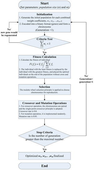
Figure 1.
The flowchart of determining combined weight coefficients by a genetic algorithm.
- Step 1
- Initialization. Generate the initial population for each combined weight coefficient, , with population size (n = 30). Then, these combined weight coefficients, , are encoded into a binary format, and are represented by a chromosome composed of “genes” of binary numbers. Each chromosome has (m − 1) genes, and each gene has 8 bits, i.e., the chromosome contains 8 × (m − 1) bits. would be calculated by .
- Step 2
- Criteria Test. Some of the population generated in Step 1 could not meet the constraint (based on Equation (23), right now, only (m − 1) combined weight coefficients are considered, thus, the constraint should be as ). To keep all individuals in the population to meet the constraints, all the chromosomes in the population are decoded into a decimal format to receive the associated real values. If the new constraint could not be met, the new gene would be regenerated for that chromosome until the constraint is met.
- Step 3
- Fitness Calculation. Due to looking for minimum forecasting residuals (the objective function), individuals with small values of the objective function always have greater fitness. Therefore, define the sum of accumulated countdown (SAC) of all individuals’ objective function values as Equation (25):where is the objective function value of the ith single forecasting model.Then, calculate the fitness of individual, , by Equation (26):At the same time, the individual with the least fitness is replaced by the individual with the greatest fitness, and placed the optimal individuals at the end of the population without cross and mutation operations.
- Step 4
- Selection. The roulette wheel selection principle is applied to choose chromosomes for reproduction, and individuals are selected for further operations.
- Step 5
- Crossover and Mutation Operations. For crossover operation, the chromosomes are paired randomly, and the proposed scheme adopts the single-point-crossover principle. Segments of paired chromosomes between two determined break-points are swapped. For mutation operation, it is implemented randomly. In this paper, the rates of crossover and mutation operations are set as 0.8 and 0.05 [36,37], respectively.
- Step 6
- Stop Criteria. If the number of generations is greater than a given scale, then, the best chromosome is determined, and the combined weight coefficients, , are also finalized; otherwise, go back to Step 1 and continue searching the next iteration.
2.4. The Total Procedure of the GM-S-SIGM-GA Model
The total procedure of the proposed GM-S-SIGM-GA model is illustrated in Figure 2. The red circle noted in Figure 2 demonstrates that the constant value effect makes the GM(1,1) robust, and the noted blue circle represents a linear function, which is simple and adaptive. However, there is a problem of adaptive over-fitting. Long-term forecasting will experience large deviations when the overall energy policy is unchanged. It needs to be corrected by using the GM(1,1)’s robustness, therefore, the use of a combined model is appropriate. In view of the intrinsic shortcomings of the GM(1,1), long-term forecasting must be corrected with the lag effect of energy policies to comprehensively reveal the regulation of natural gas consumption changes. Considering that the trigonometric function has the characteristics of frequency spectrum and phase lag, we decide to employ the concept of the trigonometric function to calculate the annual share of the natural gas consumption from the total energy consumption. The detailed procedure of the proposed GM-S-SIGM-GA model is briefed as follows:
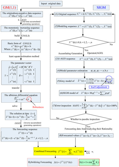
Figure 2.
The full flowchart of GM-S-SIGM-GA model.
- Step 1
- GM(1,1) and SIGM are modeled simultaneously. The training data of the collected annual natural gas dataset (from 2002 to 2010) are used to construct these two models and generate the simulation results. Please refer to Section 2.1 and Section 2.2 to learn more details about the modeling processes of these two models.
- Step 2
- GA is then employed to determine the combined weight coefficients, w. For these two modeled grey-based models, GM(1,1) and SIGM, construct the combined model, namely, the GM-SIGM-GA model, and apply the GA’s operations (selection, crossover, and mutation) to determine the most suitable combined weight coefficients. Please refer to Section 2.2 to learn more detail about the modeling process of the GM-SIGM-GA model.
- Step 3
- The annual share changing ratio is applied to adjust the effects of energy policy change every fixed period. The changes of annual shares of the natural gas consumption from the total energy consumption is taken into account to finish the final part of the proposed model, namely, the GM-S-SIGM-GA model. Please refer Section 3.3.2 to learn more details about the special adjustment mechanism.
3. Numerical Examples of the Proposed Model
3.1. Materials (Dataset of Numerical Examples)
To illustrate the superiority of the GM-SIGM-GA model, this paper employs annual natural gas consumption (billion m3) in China, from 2002 to 2017 [38], as shown in Table 1. The used annual natural gas consumption data contains, in total, 16 annual consumption values, in which the real data from 2002 to 2010, i.e., only nine data samples, are used for modeling; the real data from 2011 to 2017 are kept to verify the forecasting performance (accuracy).

Table 1.
Annual natural gas consumption in China from 2002 to 2017 (billion m3).
3.2. Forecasting Accuracy Indexes and Forecasting Accuracy Significance Tests
For forecasting accuracy measurement, three forecasting accuracy evaluation indices are used to compare the forecasting performances for each model: (1) the mean absolute percentage error (MAPE); (2) the root mean square error (RMSE); and (3) the mean absolute error (MAE). These three indices could be calculated by Equations (27)–(29), respectively:
where N is the total number of data; is the actual electric load value at point i; and is the forecasted electric load value at point i.
In addition, recommended by Lewis [39] and also employed in Ma and Liu [2], the benchmark of accuracy evaluation based on the index values of MAPE, as listed in Table 2, is also used in this paper for forecasting accuracy evaluation.
Table 2.
Benchmark of forecasting accuracy evaluation by Lewis [39].
On the other hand, to demonstrate the significant superiority of the proposed GM-SIGM-GA model, as suggested by Diebold and Mariano’s [40], Wilcoxon signed-rank test [41] is employed in this paper.
The Wilcoxon signed-rank test is often applied for small data sample sizes to compare the significant differences between two pairs of datasets (i.e., with the same size). Let be the ith pair difference of the ith pair-forecasting error, the differences would be recognized as “+” or “−” based on their values. If the value is positive, i.e., the value of first model is larger than the second one, then, mark it as “”, else, mark it as “”. Of course, if , this jth pair would be removed, then, the sample size would also be reduced. The statistic, W, of the Wilcoxon signed-rank test is illustrated as Equation (30):
Then, the decision rules of the Wilcoxon signed-rank test are as follows: If W is smaller than, or equal, to the criterion of Wilcoxon distribution under its associate degrees of freedom, then, the null hypothesis, i.e., assume that the performances of these two compared models are equal, could not be accepted. It also implies either the proposed model is significantly superior to the other model or not. If the comparing size is larger than the critical size, the Wilcoxon distribution would approximate to the normal distribution, then, the relevant statistic and associate p-value would be shown accordingly.
3.3. Forecasting Results and Improvement Analysis
3.3.1. Forecasting Results
Three models, the GM(1,1) from Wu et al. [42], the SIGM from Zeng and Li [1], and the proposed GM-SIGM-GA model, have been modeled by MATLAB software (MATLAB R2018a, under the Windows 10 version 1803 operating system, with a 3.2 GHz six-core CPU, 8 GB DRAM, and a single-chip processor as the GPU) to receive their parameters, respectively. The parameters of the GM(1,1) are determined as = 0.1556, = 28.7407; the parameters of the SIGM are verified as = 0.1241, = 2.7871, and = 21.1795. Then, based on these obtained parameters, and the actual natural gas consumption values of China in 2002–2010, the simulation values of the GM(1,1) and the SIGM are put into the GM-SIGM-GA model to calculate the combined weight coefficients, and . Figure 3 demonstrates the searching process of the combined weight coefficients, and by employing GA. In Figure 3, each colorful point implies each iteration in the GA optimization searching process. The optimal solution is indicated as and , respectively. The GA optimization process ensure the minimal forecasting error of the GM-SIGM-GA model.
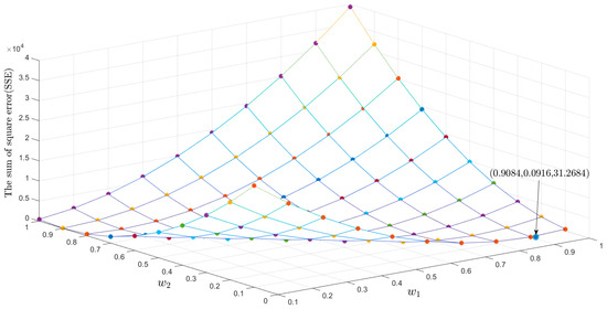
Figure 3.
The searching process of the combined weight coefficients, and by employing GA.
Based on the optimized combined weight coefficients, and , the simulation results of the GM-SIGM-GA model are obtained. The simulation results of the other two models, GM(1,1) and SIGM, and three accuracy indices of these three models from 2002 to 2010 are demonstrated in Table 3. It clearly indicates that the three models attain almost the same forecasting performances. Meanwhile, based on Lewis’s accuracy evaluation table (i.e., Table 2), the three models could all be recognized as “highly accurate” level. Furthermore, Table 4 illustrates the forecasting results and three accuracy indices of these three models from 2011 to 2017. It is obviously to learn about that, from 2011 to 2014 (i.e., the forecasting period length is within four years), the proposed model has superior forecasting performances among these three models, i.e., the MAPE value of the GM-SIGM-GA model is the best one from 2011 to 2014. However, as the forecasting period length is longer than four years, i.e., the national energy policy may have been reviewed and renewed, the GM-SIGM-GA model could only outperform the SIGM, but it could not guarantee to be the best one, i.e., the MAPE value of the GM(1,1) is superior to the MAPE value of the GM-SIGM-GA model from 2011 to 2017. By the way, based on Lewis’s table, the GM-SIGM-GA in forecasting stage could be still recognized as “highly accurate” level, it can obviously improve the forecasting inaccuracy from the SIGM.
Table 3.
The simulation results and three accuracy indices of the GM(1,1), the SIGM, and GM-SIGM-GA model.
Table 4.
The forecasting results and three accuracy indices of the GM(1,1), the SIGM, and GM-SIGM-GA model.
The simulation curves and the forecasting curves for these three models, including the GM(1,1), the SIGM, and the GM-SIGM-GA model and actual values are shown as in Figure 4a; the forecasting errors (MAPE values) for each model are shown in Figure 4b. Figure 4 also completely demonstrates the superiority of the proposed GM-SIGM-GA model.
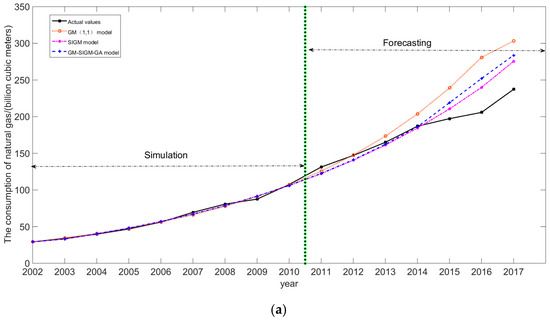
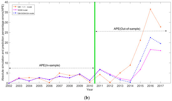
Figure 4.
(a) The simulation and forecasting results of GM(1,1), SIGM, and GM-SIGM-GA models. (b) The forecasting errors (MAPE) of GM(1,1), SIGM, and GM-SIGM-GA models.
3.3.2. Improvement Analysis
As mentioned in Section 3.3.1, it is obvious to learn about that while the forecasting period length is longer than four years, and the superior forecasting performances of the proposed GM-SIGM-GA model is declining. This is a common phenomenon when handling small sample datasets and limited information. It could be caused by the national energy policy being reviewed or renewed, and caused by the changes of the relevant operational mechanism. Therefore, the proposed GM-SIGM-GA model could not capture the regulation of the changed operational mechanism or the renewed energy policy well, even if it is intelligently combined with a genetic algorithm.
However, these changes of the influencing factors could not mutate suddenly, there should be some characteristic changes in the earlier time period. In order to simultaneously consider and extract these characteristics or features, this paper applies the share function of the natural gas consumption from the total energy consumption per year as the correction factor between the GM(1,1) and the SIGM, and proposes a coupling model with the original proposed GM-SIGM-GA model, namely GM-S-SIGM-GA model.
The changes () of annual shares of the natural gas consumption from the total energy consumption in China (from 2002 to 2016) are demonstrated in Figure 5. It is obvious that the annual share is increased from 2003 to 2006, and fluctuated heavily during 2011 to 2014, i.e., the change cycle length is 4, as mentioned above. This implies that the annual share of natural gas consumption should be a major part of China’s energy regulation, as it would be affected by other factors, such as energy price and pollution control efforts. Therefore, we propose the coefficient of adjustment, S, and define as Equation (31):
where , it implies the change ratio of two annual shares; ; .
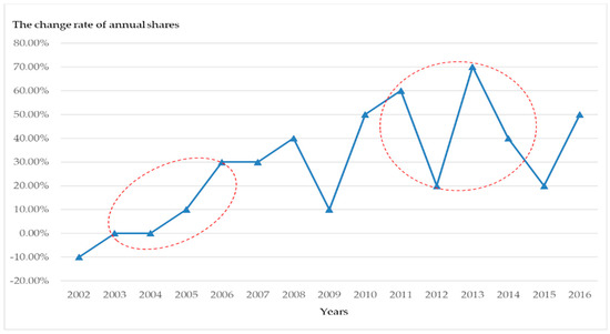
Figure 5.
The change tendency () of the annual shares of the natural gas consumption from the total energy consumption in China from 2002 to 2016.
Therefore, the proposed GM-S-SIGM-GA model is modified by S (Equation (31)) with (Equation (21)), as shown in Equation (32):
The calculation processes of the new proposed GM-S-SIGM-GA model are demonstrated completely in Table 5. It clearly indicates that the GM-S-SIGM-GA model can not only take advantage of these two models, GM(1,1) and SIGM, but cane also employ, quite well, the regulation of the change tendency of the annual shares of the natural gas consumption from the total energy consumption in China, and successfully couple these two models to play their roles excellently. Figure 6a illustrates the simulation curves and the forecasting curves for these models, including GM(1,1), SIGM, GM-SIGM-GA, and GM-S-SIGM-GA models and actual values; the forecasting errors (APE values per year) for each model are shown in Figure 6b. Figure 6 also illustrates the superiority of the GM-S-SIGM-GA model among these GM-SIGM-based models.
Table 5.
The calculation processes of the GM-S-SIGM-GA model.
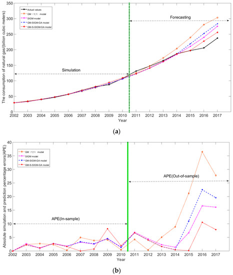
Figure 6.
(a) The simulation and forecasting results of GM(1,1), SIGM, GM-SIGM-GA, and GM-S-SIGM-GA models. (b) The forecasting errors (APE) of GM(1,1), SIGM, GM-SIGM-GA, and GM-S-SIGM-GA models.
To further compare the forecasting results of the proposed GM-S-SIGM-GA model with other grey-based models, two grey-based models, namely, the discrete grey model (briefed as DGM(1,1) [43]) and the event difference grey model (briefed as EDGM [44]), are employed. Table 6 summarizes the forecasting results of the GM-S-SIGM-GA, GM-SIGM-GA, GM(1,1), SIGM, DGM(1,1), and EDGM models. Figure 7a demonstrates the additional comparisons in terms of the simulation curves and the forecasting curves, with two other grey-based models, including the (1,1), EDGM, GM-SIGM-GA, and GM-S-SIGM-GA models and actual values; the forecasting errors (APE values per year) for each model are also shown in Figure 7b. Figure 7 completely illustrates the superiority of the GM-S-SIGM-GA model for all grey-based representative models.
Table 6.
The forecasting results of the GM(1,1), SIGM, GM-SIGM-GA, GM-S-SIGM-GA, DGM(1,1), and EDGM models.
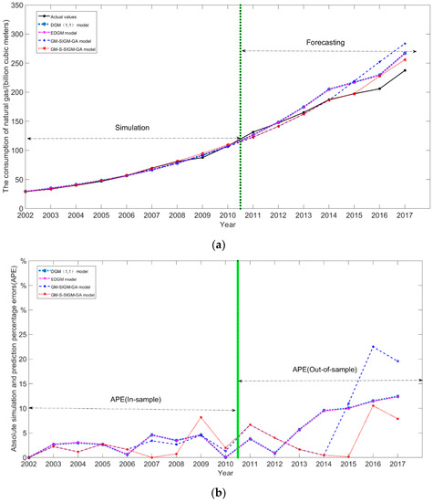
Figure 7.
(a) The simulation and forecasting results of DGM(1,1), SIGM, GM-SIGM-GA, and GM-S-SIGM-GA models. (b) The forecasting errors (APE) of DGM(1,1), EDGM, GM-SIGM-GA, and GM-S-SIGM-GA models.
Finally, to ensure the significant improvements of forecasting accuracy for the proposed GM-S-SIGM-GA model, the Wilcoxon signed-rank test is conducted, where the Wilcoxon signed-rank test is implemented under two significant levels, α = 0.025 and α = 0.05, by a two-tail test. The test results are illustrated in Table 7, showing that the proposed GM-S-SIGM-GA model has statistical significance compared to other models.
Table 7.
Results of Wilcoxon signed-rank test.
3.4. Discussions
From Table 6, it is clear to see that the proposed GM-S-SIGM-GA model receives the highest forecasting accuracy then other compared models, such as GM(1,1) [42], SIGM [1the DGM (1,1) [43], and EDGM [44] models. Firstly, the GM-SIGM-GA model is not always superior to GM(1,1) and SIGM, even when it has employed GA to intelligently determine the most suitable combined weight coefficients. However, the changes of the relevant operational mechanism from the reviewed/renewed energy policy are hardly learned or captured by the GA due to too small a data size in China’s current natural gas market. Therefore, the GM-SIGM-GA model could guarantee, with some difficulty, the superior forecasting performances.
Secondly, the proposed annual share changing tendency mechanism of the natural gas consumption from the total energy consumption could overcome the shortcoming from energy policy changes. Comparing with the GM-SIGM-GA model, the forecasting accuracy of the proposed GM-S-SIGM-GA model has been improved 4.92% (=9.40% − 4.48%). Furthermore, from Figure 6a,b, the forecasting curve of the proposed GM-S-SIGM-GA model is the closest to the actual natural gas consumption and the smallest forecasting error since the national energy policy was renewed in 2011. This comparison results reveal the superiority of the proposed annual share changing tendency mechanism, and it fills the existing gap of the grey-based models that are unable to capture the changes of the renewed/reviewed energy policy. The superior forecasting results could also provide meaningful guidelines for national energy policy-makers and electricity utility companies, to learn about the possible growth tendency of natural gas consumption by calculating the annual share changes mentioned in Equation (31), and prepare the relevant respondent actions to ensure the clean energy supply strongly support its beneficiaries, i.e., all economical activities in China.
Finally, some limitations of this paper should also be indicated. Due to the national policy, the consumption data of natural gas in China has been available since 2001 [1], thus, it limits this research to explore more interesting results, such as the differences between the short-term and the long-term, and the cyclic or seasonal tendency changes of natural gas consumption.
4. Conclusions
Along with the high growth rate of the economy in China, clean energy, like natural gas, has played an important role in national environmental management policy, thus, to accurately forecast the demand of natural gas is also an essential issue in China. This paper proposes a novel combined grey-based annual natural gas consumption forecasting model, by combining the GM(1,1) and the SIGM with genetic algorithm and the annual share changing tendency mechanism of the natural gas consumption from the total energy consumption, namely GM-S-SIGM-GA model. The experimental results indicate that the proposed GM-S-SIGM-GA model significantly outperforms to other grey-based forecasting models.
This paper firstly analyzes the embedded drawbacks of the GM(1,1) and the SIGM, and employs GA to propose the combined model, namely GM-SIGM-GA model, to determine well the suitable values of the combined weight coefficients. From Table 3, it slightly receives the highest forecasting accuracy in terms of MAPE (2.19%), RMSE (1.86), and MAE (1.48) in the simulation stage (from 2002 to 2010).
Secondly, this paper proposed annual share changing tendency mechanism with GM-SIGM-GA model, namely GM-S-SIGM-GA model, to overcome the national energy policy changes every four years. From Table 4, the proposed GM-S-SIGM-GA model outperforms other compared grey-based models, and receives the highest forecasting accuracy in terms of MAPE (4.48%), RMSE (11.59), and MAE (8.41). In addition, the forecasting performances of the proposed GM-S-SIGM-GA model also receive the statistical significance under 97.5% and 95% confident levels, respectively.
This paper demonstrates the superiorities of the GA and the annual share changing tendency mechanism. They could also be widely applied in the relevant forecasting problems. Thus, the two future research directions should be noticed. For the combined forecasting model, a great deal of potential evolutionary algorithms could be explored for their feasibility to replace GA to look for more satisfying results. On the other hand, since energy policy is often reviewed or renewed in a short-term period, the mechanism and the regulation will also be changed with time. Therefore, it requires some useful adjusting factors to modify. Looking for more powerful explanation factors to comprehensively reveal the impact mechanisms of energy policy changes will be the future research direction, such as the annual share changes or seasonal changing tendency mechanism.
Author Contributions
G.-F.F. collected the data and conceived the experiments; A.W. performed and analyzed the experiments; and W.-C.H. conceived, designed the experiments, and wrote the paper.
Funding
This research was funded by Science and Technology of Henan Province of China (no. 182400410419), The Foundation for Fostering the National Foundation of Pingdingshan University (no. PXY-PYJJ-2016006); Jiangsu Distinguished Professor Project (no. 9213618401), Jiangsu Normal University, Jiangsu Provincial Department of Education, China.
Acknowledgments
Guo-Feng Fan thanks the support from the project grants: Science and Technology of Henan Province of China (no. 182400410419), and The Foundation for Fostering the National Foundation of Pingdingshan University (no. PXY-PYJJ-2016006); Wei-Chiang Hong thanks the support from Jiangsu Distinguished Professor Project (no. 9213618401), Jiangsu Normal University, Jiangsu Provincial Department of Education, China.
Conflicts of Interest
The authors declare no conflict of interest.
Nomenclature
| the original time series | |
| the element of | |
| the first order accumulating generation operator of | |
| the element of | |
| the mean sequence of | |
| the element of | |
| a | the coefficient of development |
| b | the amount of grey action |
| u | the vector of a and b |
| c | the constant to expand from GM(1,1) to SIGM |
| the first parameter of the estimator of SIGM | |
| the second parameter of the estimator of SIGM | |
| the last parameter of the estimator of SIGM | |
| the combined weight coefficients | |
| the forecasting residual | |
| the objective function value of the ith single forecasting model | |
| the fitness of individual | |
| the changes of annual shares of the natural gas consumption from the total energy consumption | |
| S | the coefficient of adjustment (annual share changes) |
| the change ratio of two annual shares of the natural gas consumption from the total energy consumption | |
| the ith pair difference of the ith pair-forecasting error | |
| the value of is positive | |
| the value of is negative | |
| W | the statistic of the Wilcoxon signed-rank test |
References
- Zeng, B.; Li, C. Forecasting the natural gas demand in China using a self-adapting intelligent grey model. Energy 2016, 112, 810–825. [Google Scholar] [CrossRef]
- Ma, X.; Liu, Z. Application of a novel time-delayed polynomial grey model to predict the natural gas consumption in China. J. Comput. Appl. Math. 2017, 324, 17–24. [Google Scholar] [CrossRef]
- Bahrami, S.; Sheikhi, A. From demand response in smart grid toward integrated demand response in smart energy hub. IEEE Trans. Smart Grid 2016, 7, 650–658. [Google Scholar] [CrossRef]
- Sheikhi, A.; Rayati, M.; Bahrami, S.; Ranjbar, A.M.; Sattari, S. A cloud computing framework on demand side management game in smart energy hubs. Int. J. Electr. Power Energy Syst. 2015, 64, 1007–1016. [Google Scholar] [CrossRef]
- Amini, M.H.; Boroojeni, K.G.; Iyengar, S.S.; Blaabjerg, F.; Pardalos, P.M.; Madni, A.M. A panorama of future interdependent networks: From intelligent infrastructures to smart cities. In Sustainable Interdependent Networks; Amini, M., Boroojeni, K., Iyengar, S., Pardalos, P., Blaabjerg, F., Madni, A., Eds.; Springer: Cham, Switzerland; New York, NY, USA, 2018; Volume 145, pp. 1–10. ISBN 978-3-319-74411-7. [Google Scholar]
- Ding, S.; Hipel, K.W.; Dang, Y. Forecasting China’s electricity consumption using a new grey prediction model. Energy 2018, 149, 314–328. [Google Scholar] [CrossRef]
- Ervural, B.C.; Beyca, O.F.; Zaim, S. Model estimation of ARMA using genetic algorithms: A case study of forecasting natural gas consumption. Procedia Soc. Behav. Sci. 2016, 235, 537–545. [Google Scholar] [CrossRef]
- Yuan, C.Q.; Liu, S.F.; Fang, Z.G. Comparison of China’s primary energy consumption forecasting by using ARIMA (the autoregressive integrated moving average) model and GM (1, 1) model. Energy 2016, 100, 384–390. [Google Scholar] [CrossRef]
- Wadud, Z.; Himadri, S.; Dey, H.S.; Kabir, M.A.; Khan, S.I. Modeling and forecasting natural gas demand in Bangladesh. Energy Policy 2011, 39, 7372–7380. [Google Scholar] [CrossRef]
- Özmen, A.; Yılmaz, Y.; Weber, G.-W. Natural gas consumption forecast with MARS and CMARS models for residential users. Energy Econ. 2018, 70, 357–381. [Google Scholar] [CrossRef]
- Bianco, V.; Scarpa, F.; Tagliafico, L.A. Scenario analysis of nonresidential natural gas consumption in Italy. Appl. Energy 2014, 113, 392–403. [Google Scholar] [CrossRef]
- Forouzanfar, M.; Doustmohammadi, A.; Menhaj, M.B.; Hasanzadeh, S. Modeling and estimation of the natural gas consumption for residential and commercial sectors in Iran. Appl. Energy 2010, 87, 268–274. [Google Scholar] [CrossRef]
- Shaikh, F.; Ji, Q. Forecasting natural gas demand in China: Logistic modelling analysis. Int. J. Electr. Power Energy Syst. 2016, 77, 25–32. [Google Scholar] [CrossRef]
- Zhang, W.; Yang, J. Forecasting natural gas consumption in China by Bayesian model averaging. Energy Rep. 2015, 1, 216–220. [Google Scholar] [CrossRef]
- Yuan, X.-C.; Sun, X.; Zhao, W.; Mi, Z.; Wang, B.; Wei, Y.-M. Forecasting China’s regional energy demand by 2030: A Bayesian approach. Resour. Conserv. Recycl. 2017, 127, 85–95. [Google Scholar] [CrossRef]
- Szoplik, J. Forecasting of natural gas consumption with artificial neural networks. Energy 2015, 85, 208–220. [Google Scholar] [CrossRef]
- Azadeh, A.; Asadzadeh, S.M.; Saberi, M.; Nadimi, V.; Tajvidi, A.; Sheikalishahi, M. A Neuro-fuzzy-stochastic frontier analysis approach for long-term natural gas consumption forecasting and behavior analysis: The cases of Bahrain, Saudi Arabia, Syria, and UAE. Appl. Energy 2011, 88, 3850–3859. [Google Scholar] [CrossRef]
- Kaynar, O.; Yilmaz, I.; Demirkoparan, F. Forecasting of natural gas consumption with neural network and neuro fuzzy system. Energy Educ. Sci. Technol. Part A Energy Sci. Res. 2011, 26, 221–238. [Google Scholar]
- Potočnik, P.; Soldo, B.; Šimunović, G.; Šarić, T.; Jeromen, A.; Govekar, E. Comparison of static and adaptive models for short-term residential natural gas forecasting in Croatia. Appl. Energy 2014, 129, 94–103. [Google Scholar] [CrossRef]
- Karadede, Y.; Ozdemir, G.; Aydemir, E. Breeder hybrid algorithm approach for natural gas demand forecasting model. Energy 2017, 141, 1269–1284. [Google Scholar] [CrossRef]
- Panapakidis, I.P.; Dagoumas, A.S. Day-ahead natural gas demand forecasting based on the combination of wavelet transform and ANFIS/genetic algorithm/neural network model. Energy 2017, 118, 231–245. [Google Scholar] [CrossRef]
- Rodger, J.A. A fuzzy nearest neighbor neural network statistical model for predicting demand for natural gas and energy cost savings in public buildings. Expert Syst. Appl. 2014, 41, 1813–1829. [Google Scholar] [CrossRef]
- Azadeh, A.; Asadzadeh, S.M.; Ghanbari, A. An adaptive network-based fuzzy inference system for short-term natural gas demand estimation: Uncertain and complex environments. Energy Policy 2010, 38, 1529–1536. [Google Scholar] [CrossRef]
- Bai, Y.; Li, C. Daily natural gas consumption forecasting based on a structure-calibrated support vector regression approach. Energy Build. 2016, 127, 571–579. [Google Scholar] [CrossRef]
- Zhu, L.; Li, M.S.; Wu, Q.H.; Jiang, L. Short-term natural gas demand prediction based on support vector regression with false neighbours filtered. Energy 2015, 80, 428–436. [Google Scholar] [CrossRef]
- Wu, Y.-H.; Shen, H. Grey-related least squares support vector machine optimization model and its application in predicting natural gas consumption demand. J. Comput. Appl. Math. 2018, 338, 212–220. [Google Scholar] [CrossRef]
- Fan, G.; Peng, L.-L.; Hong, W.-C.; Sun, F. Electric load forecasting by the SVR model with differential empirical mode decomposition and auto regression. Neurocomputing 2016, 173, 958–970. [Google Scholar] [CrossRef]
- Kaytez, F.; Taplamacioglu, M.C.; Cam, E.; Hardalac, F. Forecasting electricity consumption: A comparison of regression analysis, neural networks and least squares support vector machines. Int. J. Electr. Power Energy Syst. 2015, 67, 431–438. [Google Scholar] [CrossRef]
- Deng, J.L. Control problems of grey systems. Syst. Control Lett. 1982, 1, 288–294. [Google Scholar]
- Wang, J.; Jiang, H.; Zhou, Q.; Wu, J.; Qin, S. China’s natural gas production and consumption analysis based on the multicycle Hubbert model and rolling Grey model. Renew. Sustain. Energy Rev. 2016, 53, 1149–1167. [Google Scholar] [CrossRef]
- Shaikh, F.; Ji, Q.; Shaikh, P.H.; Mirjat, N.H.; Uqaili, M.A. Forecasting China’s natural gas demand based on optimised nonlinear grey models. Energy 2017, 140, 941–951. [Google Scholar] [CrossRef]
- Liu, X.; Moreno, B.; García, A.S. A grey neural network and input-output combined forecasting model. Primary energy consumption forecasts in Spanish economic sectors. Energy 2016, 115, 1042–1054. [Google Scholar] [CrossRef]
- Hamzacebi, C.; Es, H.A. Forecasting the annual electricity consumption of Turkey using an optimized grey model. Energy 2014, 70, 165–171. [Google Scholar] [CrossRef]
- Ma, X.; Liu, Z. The kernel-based nonlinear multivariate grey model. Appl. Math. Model. 2018, 56, 217–238. [Google Scholar] [CrossRef]
- Mehrtash, M.; Kargarian, A.; Mohammadi, A. Partition-based bus renumbering effect on interior point-based OPF solution. In Proceedings of the 2018 IEEE Texas Power and Energy Conference (TPEC), College Station, TX, USA, 8–9 February 2018; IEEE: College Station, TX, USA, 2018. [Google Scholar]
- Fan, G.-F.; Peng, L.-L.; Zhao, X.; Hong, W.-C. Applications of hybrid EMD with PSO and GA for an SVR-based load forecasting model. Energies 2017, 10, 1713. [Google Scholar] [CrossRef]
- Pai, P.-F.; Hong, W.-C. A recurrent support vector regression model in rainfall forecasting. Hydrol. Process. 2007, 21, 819–827. [Google Scholar] [CrossRef]
- The Annual Natural Gas Consumption in China. Available online: https://www.china5e.com/ (accessed on 10 May 2018).
- Lewis, C.D. Industrial and Business Forecasting Method; Butter-Worth-Heinemann: London, UK, 1982. [Google Scholar]
- Diebold, F.X.; Mariano, R.S. Comparing predictive accuracy. J. Bus. Econ. Stat. 1995, 13, 134–144. [Google Scholar]
- Wilcoxon, F. Individual comparisons by ranking methods. Biom. Bull. 1945, 1, 80–83. [Google Scholar] [CrossRef]
- Wu, L.F.; Liu, S.F.; Liu, D.L. Modeling and forecasting CO2 emissions in the BRICS (Brazil, Russia, India, China, and South Africa) countries using a novel multi-variable grey model. Energy 2015, 79, 489–495. [Google Scholar] [CrossRef]
- Xie, N.M.; Liu, S.F. Discrete grey forecasting model and its optimization. Appl. Math. Model. 2008, 33, 1173–1186. [Google Scholar] [CrossRef]
- Liu, S.F.; Yang, Y.J.; Wu, L.F. Grey Systems Theory and Applications, 7th ed.; Science Press: Beijing, China, 2014; ISBN 9787030409126. (In Chinese) [Google Scholar]


© 2018 by the authors. Licensee MDPI, Basel, Switzerland. This article is an open access article distributed under the terms and conditions of the Creative Commons Attribution (CC BY) license (http://creativecommons.org/licenses/by/4.0/).