Evaluation of the Spot Shape on the Target for Flat Heliostats

Abstract

The aim of this study is to evaluate the changes of the spot shape on the target in dependence of the variations of size and faceting of a flat heliostat or an array of heliostats. The flat heliostat, or a flat heliostat array, is a layout common for Concentation Solar Power (CSP) plants. The spot shape is evaluated by means of a numerical integration of an appropriate function; in order to confirm the results, both an analysis based on the Lagrange invariance and some simulations are performed. The first one validates the power density value in the central part of the spot, while the simulations assess the spot shape, which in its central part differs less than 3% from the calculated result. The utilized numerical method does not require specialized software or complex calculation models; it determines an accurate spot shape but cannot take into account shading and blocking phenomena.

1. Introduction

During the last years, many theoretical and experimental researches were carried out in order to increase the efficiency and the ratio benefits/costs of solar plants. Many efforts were made in order to improve optical layouts, thermal exchange systems and materials (a not very recent but comprehensive analysis is given in [1]), but researchers turned their attention also to increasing the density of the heliostat field [2,3] or to studying the dynamic of the receiver [4,5]. The correct sizing of the receiver was investigated in many scientific articles (e.g., [5]), as well as the flux distribution on the receiver [6,7]. A key point of these studies was the correct sizing of mirrors and target, also referring to multi-faceted plane mirrors that represent a useful alternative to spherical or parabolic mirrors, which are more expensive and difficult to manufacture. The shape of the spot on the target is a fundamental parameter because it strongly influences the size of the target, which has to be a trade-off between the requirements for radiation collection and energy losses [8]. The aim of the present work is to determine the spot shape on the target in a heliostat field by means of an easy but efficient mathematical analysis. The examined system is a central tower with flat or faceted heliostats, which is a common layout of commercial Concentration Solar Power (CSP) plants. The proposed methodology permits the correct sizing of the mirroring elements also taking into account the concentration limit achievable in the actual layout.

In this framework, a key element of the design phase is represented by the determination of the spot shape on the target that can be assessed in two different ways: by a raytracing (generally using a Monte-Carlo method) or by the development of a suitable analytic function [9].

The first way led to the creation of some dedicated software tools such as STRAL [10] or SolTrace [11]. In order to obtain useful results they have to trace a large number of rays, so a large processing power is requested; despite the increased performance of the computers, the raytracing requires relatively long time.

The problem of the determination of an analytical function that describes the spot shape on the receiver was studied by many authors, which very often proposed complex methods of convolution of solar divergence and errors. Among them, Elsayed and Fathalah in [12] tried to evaluate the flux density function on the receiver, but they utilized the average radiation concentration as input parameter and the angle between the adjacent sides of the principal image of the heliostat (that is the image generated only by collimated sun rays) as control parameter, which are very difficult data to evaluate. Lipps and Wanzel in [13] performed a very careful analysis for a flat polygonal heliostat, taking into account also shading and blocking phenomena. However, the beam enlargement is expressed by a polynomial approximation instead of a standard deviation value, and in general, the expression of the data is quite convoluted, requiring the calculation of the image of each single heliostat based on mirror boundaries definition. Collado et al. in [14] supplied an analytic description of the beam, but only for spherical-shaped heliostats (the convolution function in this case convolves three functions: sun shape, errors and concentration) with the receiver at suitable distance to produce the minimum circle of confusion; in this paper there is also a table with a succinct description of the characteristics of some previous works.

In this field, large efforts were devoted to develop efficient software for the evaluation of the heliostats fields. An early example was DELSOL, developed from 1979 at Sandia Laboratoires. The upgraded version, DELSOL3, is described in [15], but now it seems no longer updated [16]; this software utilizes an analytical Hermite polynomial expansion/convolution-of-moments and includes an economic analysis too. HELIOS has the same scope of DELSOL, but is more accurate and slow; in [17] is stated: “HELIOS is used where a detailed description of the heliostat is available and an extremely accurate evaluation of flux density is desired”. Both these software tools are built to evaluate the performance of a whole heliostats field, while the aim of the proposed work is to choose the correct size of heliostats in an early stage of design. Others software tools for the study of the flux distribution generated by a spherical heliostat, assuming a circular symmetry, are UNIZAR and HFLCAL, analyzed by Collado in 2010 [18]. In particular, an interesting application is the program HFLCAL, presented by P. Schwarbözl et al. at the SolarPaces 2009 conference [19], where the authors utilize a mathematical method of analysis very similar to the one shown in the present work. The difference is that HFLCAL, like UNIZAR, considers spherical faceted mirrors (with spherical curvature both on the facets and on the envelope). These assumptions lead to formulas that are to all appearances similar to the ones in the following sections of this paper, but actually they are quite different. In fact, considering the spot, in HFLCAL it always has a shape that is basically Gaussian and modified by the astigmatism.

The method utilized in this work concerns flat heliostats, which are very often employed in CSP plants with a central tower to decrease the costs [20]. The suggested approach is much simpler than the previous ones (it requires only a standard worksheet like Excel and few VBA (Visual Basic for Applications) program lines, but no dedicated software codes) and permits one to perform a useful analysis on the characteristics of the spot and on how the heliostat parameters influence them. The key elements are the approximation of the angular shape of the beam reflected by a point on the heliostat surface to a bi-dimensional Gaussian distribution (centered on the direction of the specular reflection) and its equivalence with the irradiance space distribution generated by the same beam on the target plane. Hence, the irradiance on a point of the target is calculated as the sum of the contributions from all the points of the heliostat (the atmospheric attenuation is neglected). The final results include the maximum power concentration on the spot center achievable with a faceted heliostat, the variation of the spot shape depending on the heliostat distance and the minimum size of the facets (under which no advantages arise). In order to confirm the results achieved by the mathematical analysis, a set of simulated models have been developed using a non-sequential optical computer-aided design (CAD, by Lambda Research TracePro). The use of a non-sequential optical CAD permits to evaluate the irradiance distribution on the target potentially taking into account all the physical phenomena involved (reflection, refraction, scattering …). In fact, while a sequential optical CAD, where the order in which the rays hit the surfaces is defined by the user, is dedicated to the evaluation of aberrations, in a non-sequential optical CAD the rays hit the surfaces depending on their optical path, so it is focused on the calculation of radiometric and photometric quantities as irradiance maps on the target. The non-sequential optical CADs were developed originally for illumination engineering; in [21] a short description of their characteristics is provided. Moreover, the application of Lagrange invariance confirms the results obtained from the calculation and the simulations.

2. Mathematical Analysis

This section provides a concise and precise description of the mathematical analysis. Firstly, the study considers a rectangular-shaped flat heliostat with the target on the axis. The beam angular distribution essentially depends on solar divergence, heliostat pointing errors and mirrors surface features (slope errors, gloss). The solar divergence has its peculiar shape, that can be roughly assimilated to an uniform distribution with semi-aperture 4.7 mrad [22], as well as the heliostat pointing errors ([23], mean value = 3 mrad). Regarding the mirrors surface features, the angular shape of the reflected beam is Gaussian, with standard deviation (std. dev.) σ = 5 mrad [24]. In effect, Rabl in [25] demonstrated that the error cone due to the reflection on a mirror surface is elliptical, but Guo and Wang in [26] realized an equivalence between circular and elliptical Gaussian distribution. Moreover, it has to be considered that the sun position varies during the day and the seasons, then the axes directions of the elliptical Gaussian distribution on the receiver plane greatly vary. Consequently, the assumption of a Gaussian circular distribution is more adequate to the aim of this study, which is the correct sizing of heliostats or heliostat facets in a solar plant that works on a large range of sun positions. Researchers demonstrated that in many cases the convolution between the enlargements, both intrinsic of solar light and due to the errors, can be considered as a Gaussian distribution when the first cause is less important than the second one [27]. Then, in this case it is worth to approximate the previous uniform distributions to Gaussian ones with std. dev. σ = a/√3, where a is the half width of the uniform distributions [28]. Thus, from a practical point of view the beam enlargement of the beam reflected by the heliostat field can be treated as Gaussian with std. dev. σ = 5.9 mrad [29].

If I(θ) is the intensity distribution with respect to the reflection direction and σ_θ is its standard deviation, for a single point on the heliostat surface this relation is valid [30]:

$$I\left(\theta \right)= I_{0}exp\left(-\frac{{\theta }^2}{2{\sigma }_{\theta }{}^2}\right)$$

(1)

where:

-

I₀ is the peak intensity value;

-

θ is the angle between the normal to the heliostat surface and the direction of the specular reflection;

-

σ_θ is the standard deviation of the angular distribution taking into account all the causes of beam enlargement.

It is preferable to rewrite that formula in terms of irradiance E(x, y) on the generic target point P = (x, y). Utilizing the expression E = I/d² (where d is the heliostat-target distance [31]) and expressing the angle θ of Equation (1) as a function of (x, y):

$$E\left(x,y\right)=E_{0}exp\left(-\frac{{\left(arctg\left(\frac{\sqrt{x^{2 }+ y^2}}{d}\right)\right)}^2}{2{\left(arctg\left(\frac{{\sigma }_{x,y}}{d}\right)\right)}^2}\right) \cong E_{0}exp\left(-\frac{\frac{x^2 + y^2}{d^2}}{\frac{2{\sigma }_{x,y}{}^2}{d^2}}\right)= E_{0}exp\left(-\frac{x^2 + y^2}{2{\sigma }_{x,y}{}^2}\right)$$

(2)

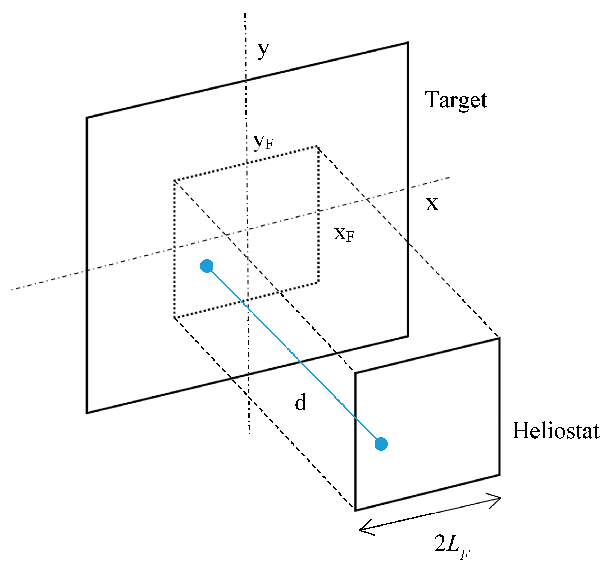
Due to the fact that a single point is considered, obviously σ_x = σ_y = σ_x,y = (σ_θ·d), where d is the distance between the heliostat and the target, indicated in Figure 1. Equation (2) is equivalent to the Equation (7) in [26] when the center of the reference system coincides with the point of maximum irradiance E₀.

The next step is to consider an extended squared heliostat; the situation is more complicated, because the convolution between a square (the heliostat surface) and the Gaussian distribution has to be taken into account. In this case, due to the integration on the surface, E_SUN (the solar irradiance on the heliostat) must substitute the E₀ constant (irradiance on the center of the target), with the suitable normalization; the actual normalization corresponds to a bi-dimensional Gaussian distribution with zero correlation between the two variables x_F and y_F [9]. For a square heliostat with side 2L_F:

$$E\left(x,y\right)= \frac{E_{SUN}}{2\pi {\sigma }_{xy}{}^2}{{\displaystyle \int }}_{-L_F}^{L_F}{{\displaystyle \int }}_{-L_F}^{L_F}exp\left(-\frac{{\left(x-x_F\right)}^2}{2{\sigma }_{x,y}{}^2}\right)exp\left(-\frac{{\left(y-y_F\right)}^2}{2{\sigma }_{x,y}{}^2}\right)d{x}_{F}d{y}_F$$

(3)

Equation (3) is similar to the Equation for a Gaussian enlargement on the target utilized by the software HFCAL (see the Equation (7) in [18]), but the total flux from the focusing heliostat in Equation (3) is replaced by the sun irradiance E_SUN with an integration of the exponential terms on the heliostat surface. From an optical point of view, it means that the irradiance on the target point (x, y) is obtained as the sum of the contributions from all the points of the flat heliostat.

Substituting:

$$t_x= \frac{x-x_F}{\sqrt{2}{\sigma }_{x,y}}$$

$$t_y= \frac{y-y_F}{\sqrt{2}{\sigma }_{x,y}}$$

The final Equation is:

$$E\left(x,y\right)= \frac{E_{SUN}}{\pi }\underset{\frac{x+L_F}{\sqrt{2}\sigma }}{\overset{\frac{x-L_F}{\sqrt{2}\sigma }}{{\displaystyle \int }}}\underset{\frac{y+L_F}{\sqrt{2}\sigma }}{\overset{\frac{y-L_F}{\sqrt{2}\sigma }}{{\displaystyle \int }}}{e}^{-t_x{}^2}{e}^{-t_y{}^2}d{t}_{x}d{t}_y$$

(4)

It is the bi-dimensional Error Function (erf) Equation (integral of Gaussian function) that does not admit analytical solution. However, it is very easy to perform a numerical integration.

3. Numerical Integration and Simulation Results

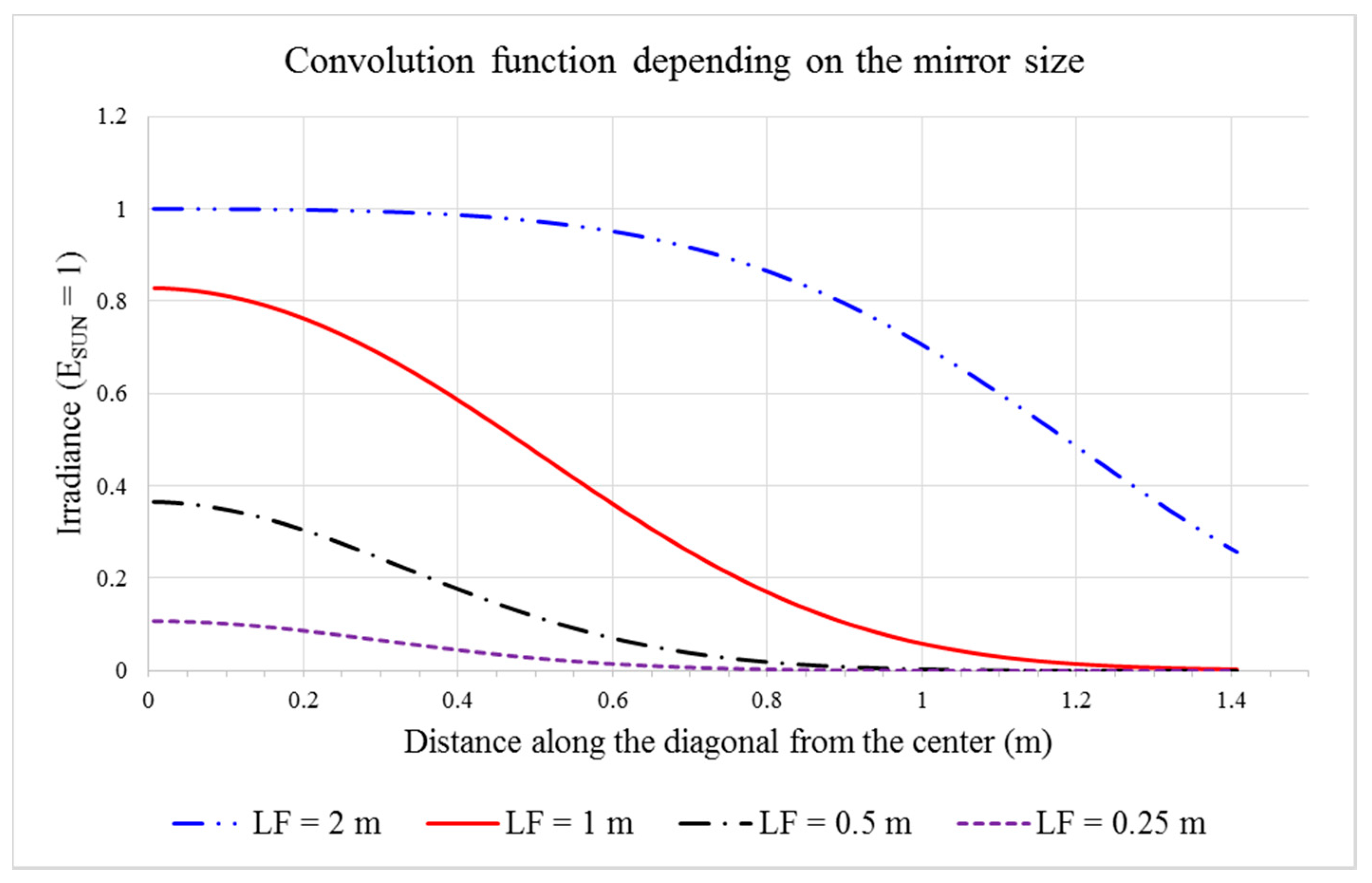
The irradiance E(x, y) on the target can be obtained by numerical integration of Equation (4). In Figure 2 the behavior of this function along the diagonal (for x = y) is shown for different values of L_F. The irradiance values are calculated for a square heliostat with side 2L_F, considering four different sizes (L_F) for the heliostat. The heliostat-target distance is 50 m, σ_x,y = 0.264 (total angular divergence = 5.9 mrad) with the E_SUN constant set to 1. Obviously in Figure 2 the curves for different values of L_F refer to different ordinate values in the center of the target, because for example the mirror with L_F = 0.25 m has area 16 times smaller than the mirror with L_F = 1 m.

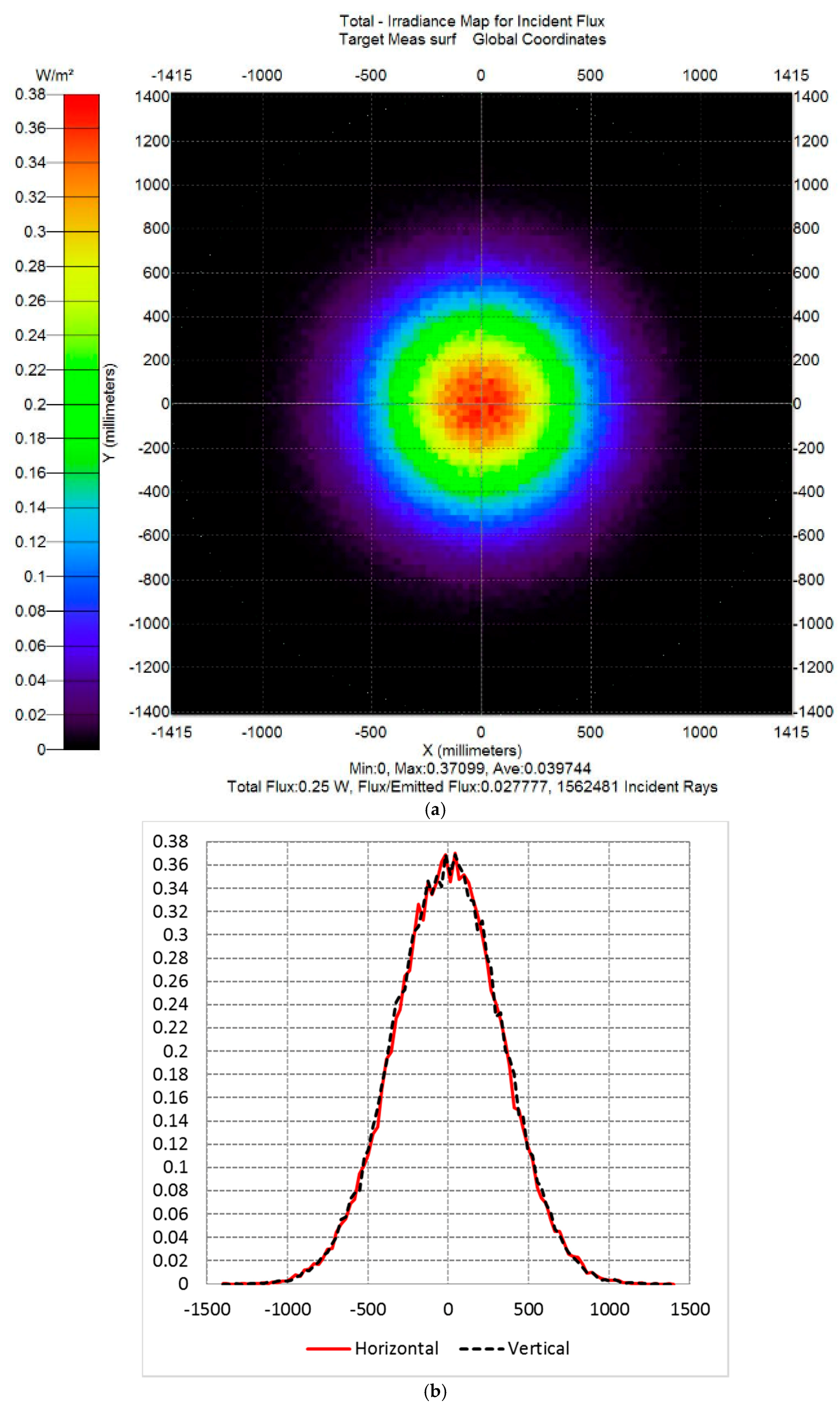
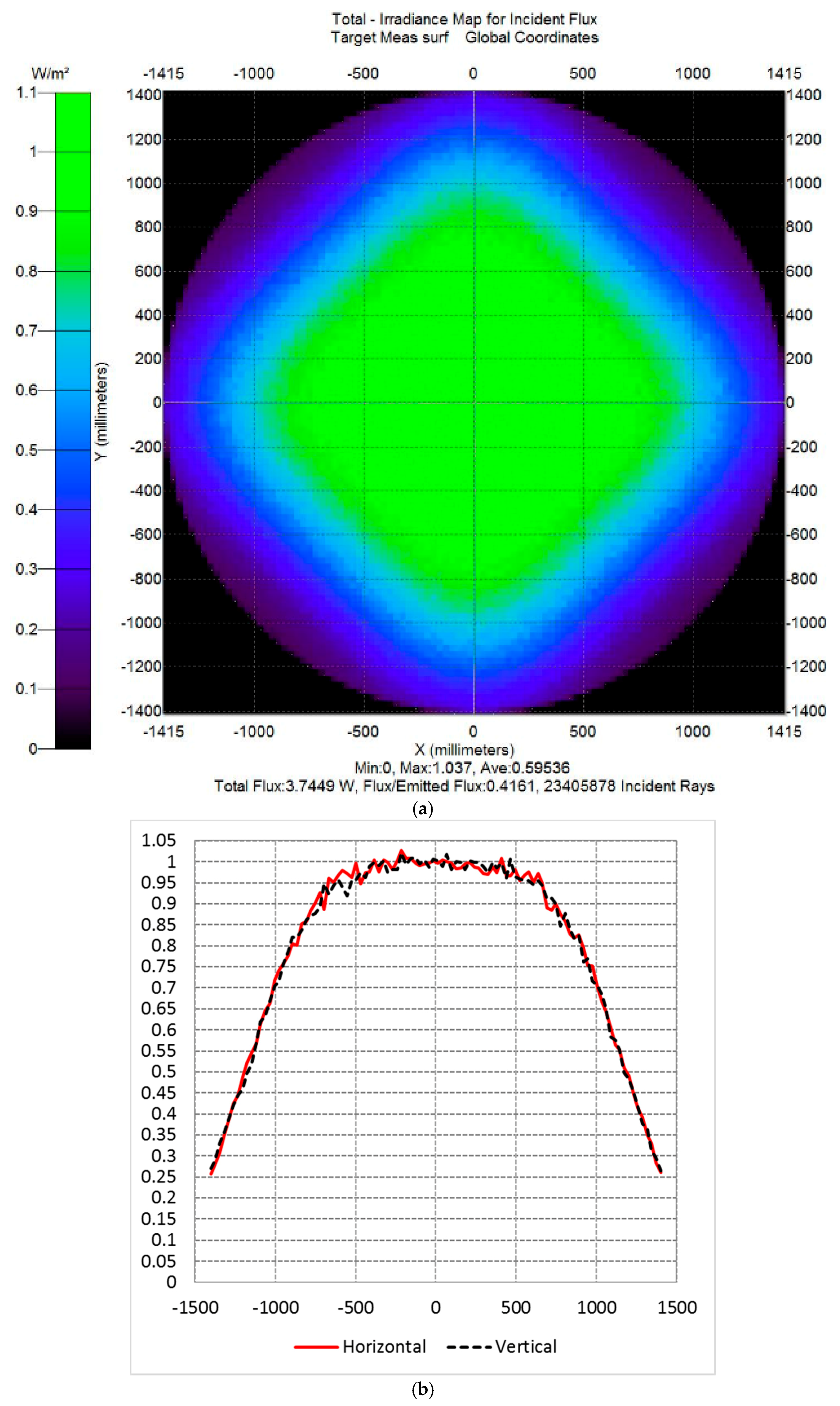
Some simulations were performed by means of TracePro (TracePro 2018 Expert Release 18.2, Lambda Research Corporation, Littleton, MA, USA), a software dedicated to lighting simulation. In the following text, “calculated results” or “calculated profiles” refer to the values obtained by the numerical integration of Equation (4), “simulated results” or “simulated shape” refer to the values obtained by TracePro raytracing. 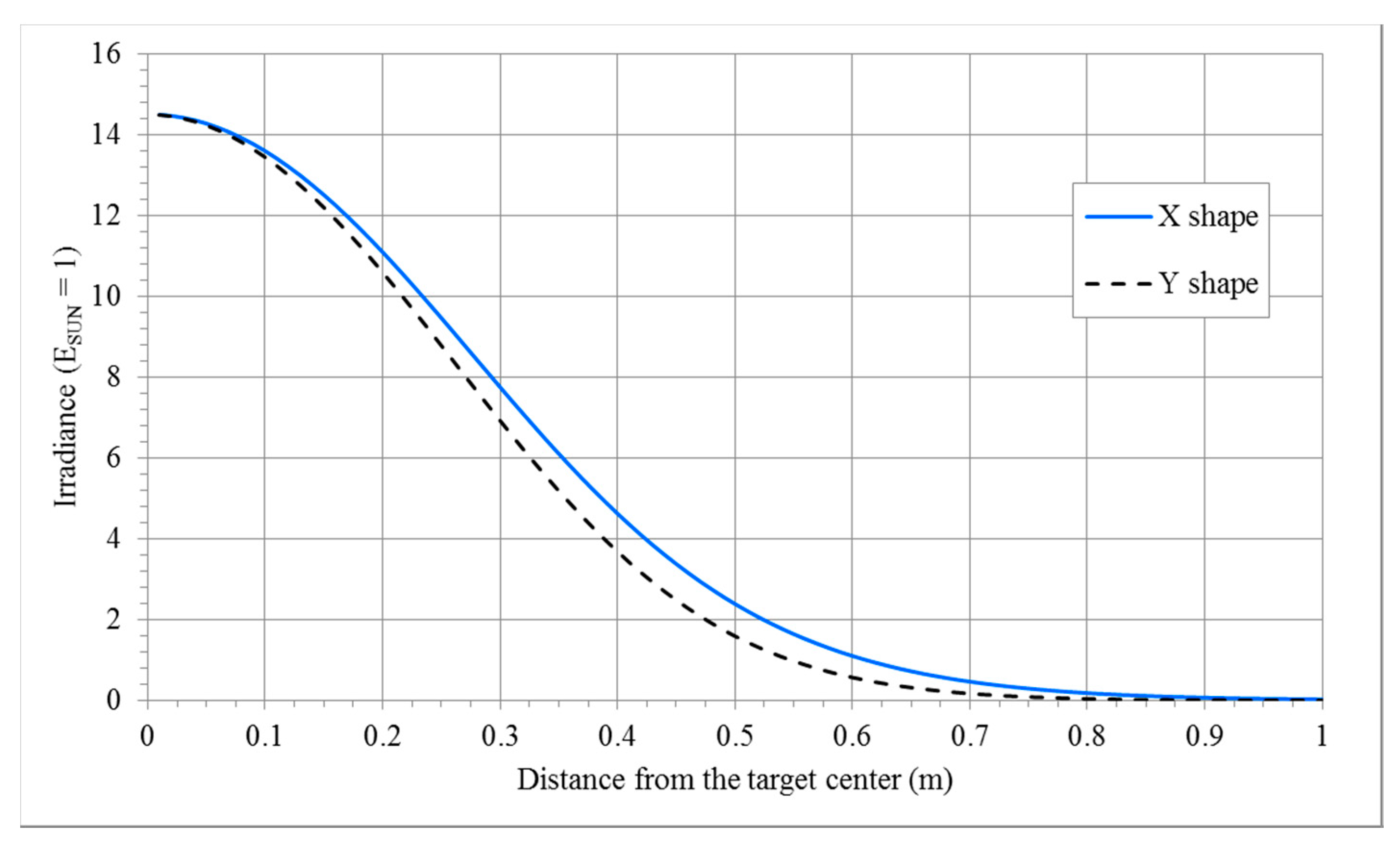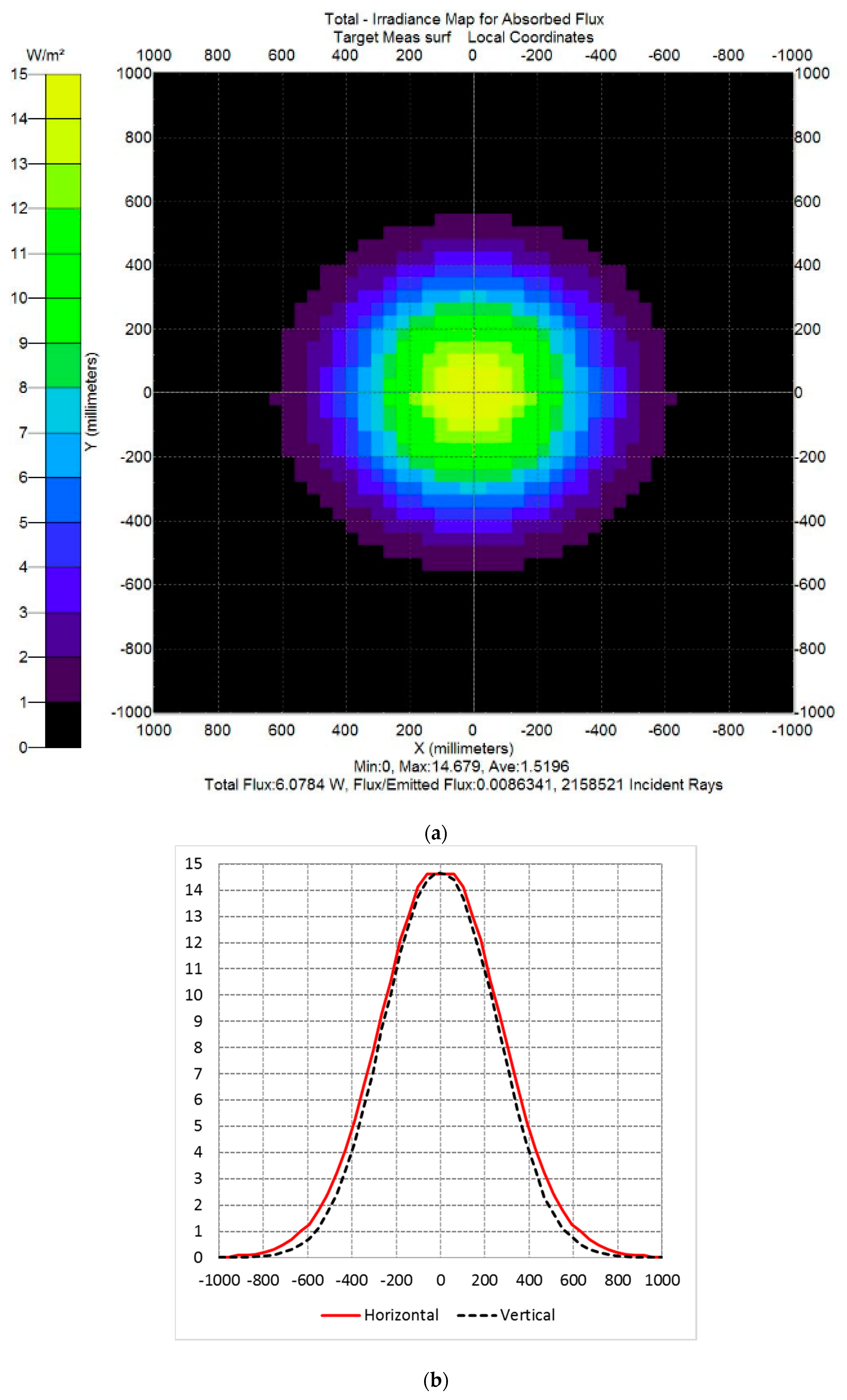The irradiance maps and profiles are presented in Figure 3 and Figure 4 for two of the examined cases. These two simulations were carried out keeping the other parameters as in the previous numerical calculation.

The target irradiance map a and the corresponding vertical/horizontal profiles b are plotted in Figure 3 for mirror side L_F = 0.5 m and in Figure 4 for L_F = 2 m.

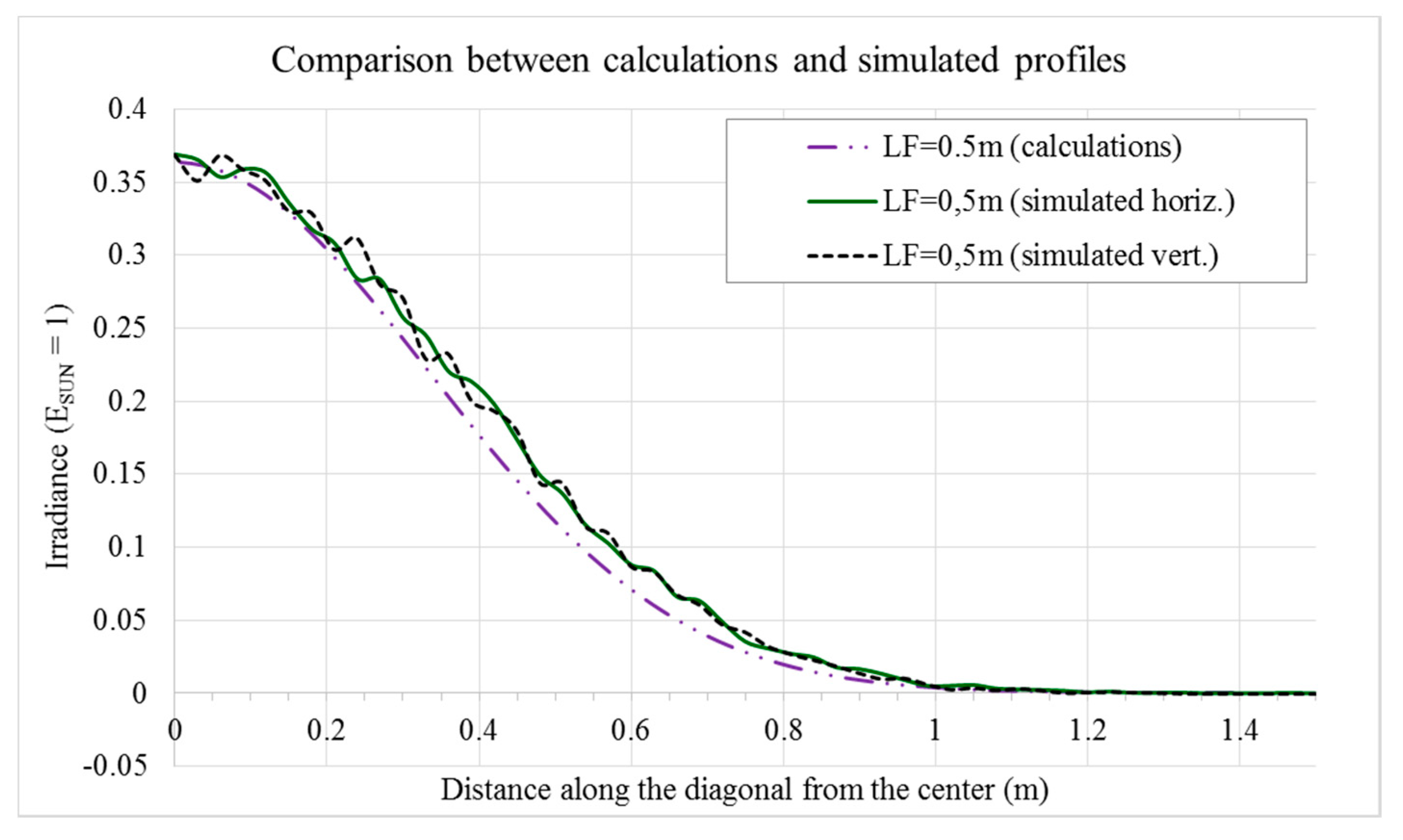
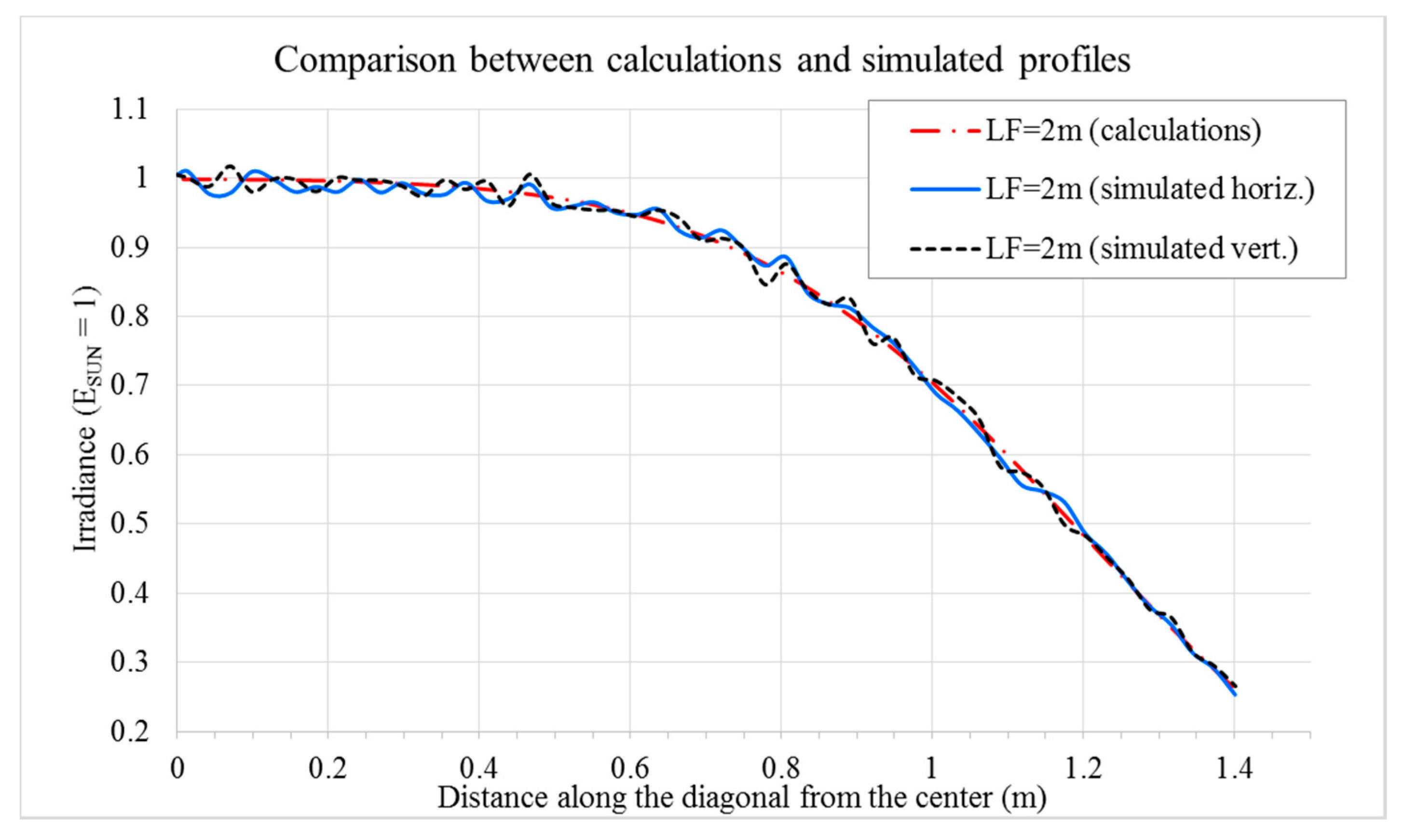
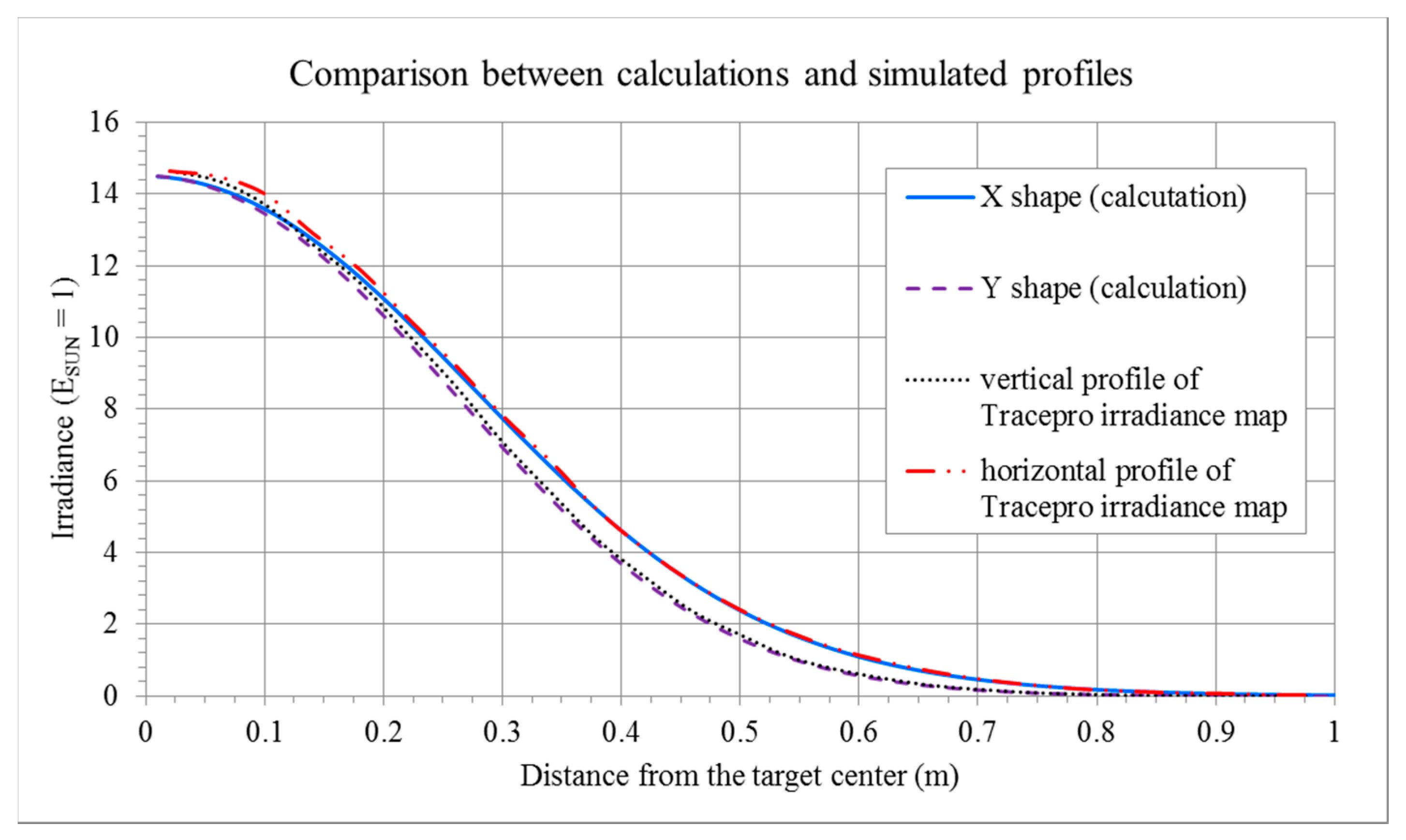
There is good agreement between the theoretical calculation results and the irradiance map profiles obtained from the TracePro simulations. Some examples of comparison are presented in Figure 5 and Figure 6, for L_F = 0.5 m (Figure 5) and for L_F = 2 m (Figure 6).

Please note the different shape of the spot on the receiver, due to the effect of the divergence.

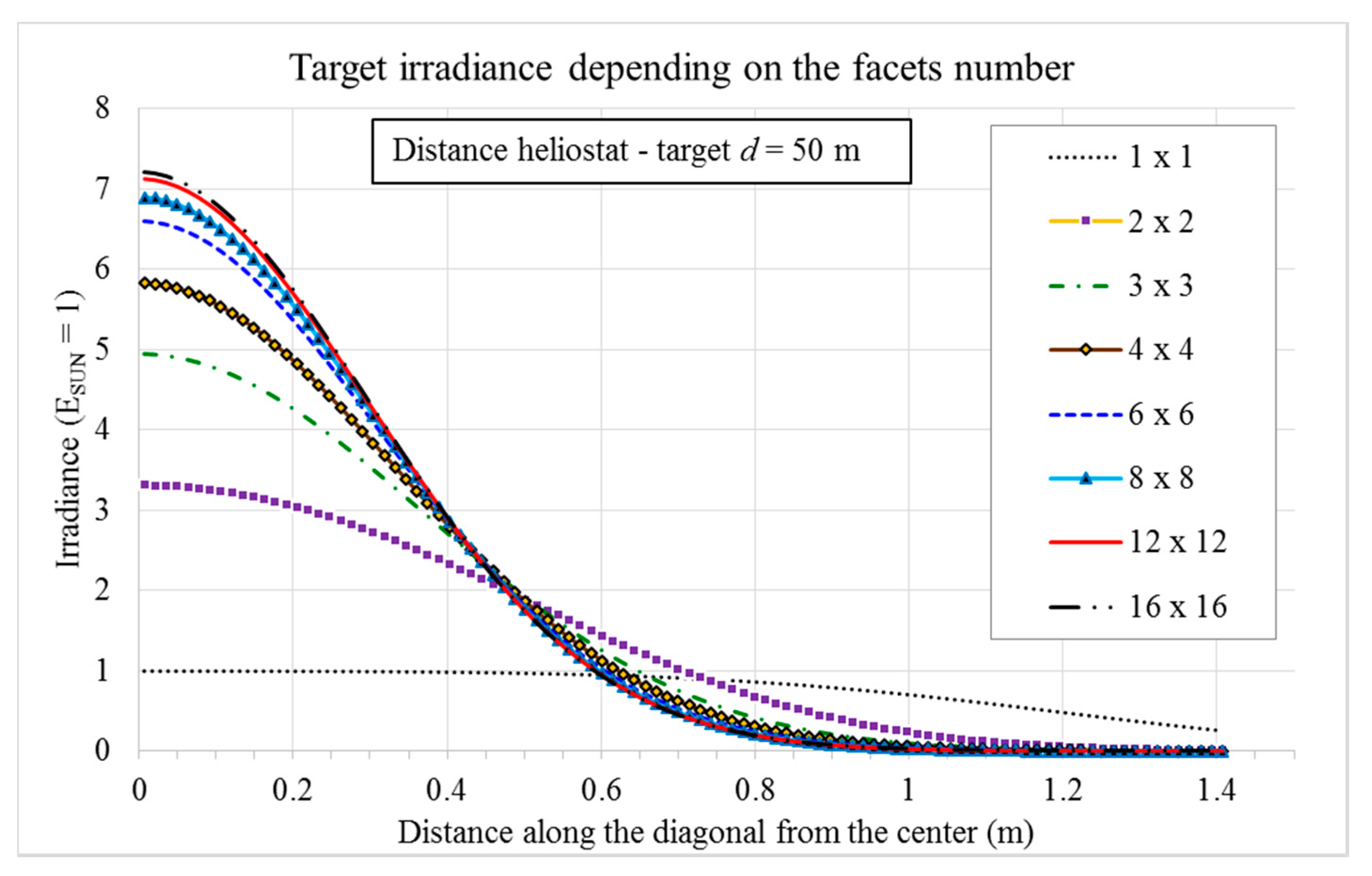
What happens with faceted mirrors is shown in Figure 7: the heliostat (formed by many mirrors) has still the same size (side 2L_F = 2 m), but the facets number changes from 1 to 256. It is supposed that all the facets lay of a spherical envelope and are oriented in order to reflect its central ray toward the center of the receiver (the little angle difference is neglected). The irradiance along the target diagonal is plotted in Figure 7 for increasing number of facets per side, from 1 up to 16 (256 facets in total).

The case of the single-facet heliostat seems different from the other curves; actually, it is in accordance with them. In fact the 1 × 1 curve is equal to the irradiance variation along the diagonal of the heliostat modified by the flux enlargement. Correctly, its maximum irradiance is E_SUN because a flat heliostat does not focus the beam. The increase of the facets number (canted towards the target) makes the faceted heliostat more and more similar to a spherical mirror focused on the target (it represents a limit case).

Please note that the areas under the curves of Figure 7 are not equal because each plotted curve is the shape of the function along a line (the diagonal), and it does not represent the energy collection on the plane.

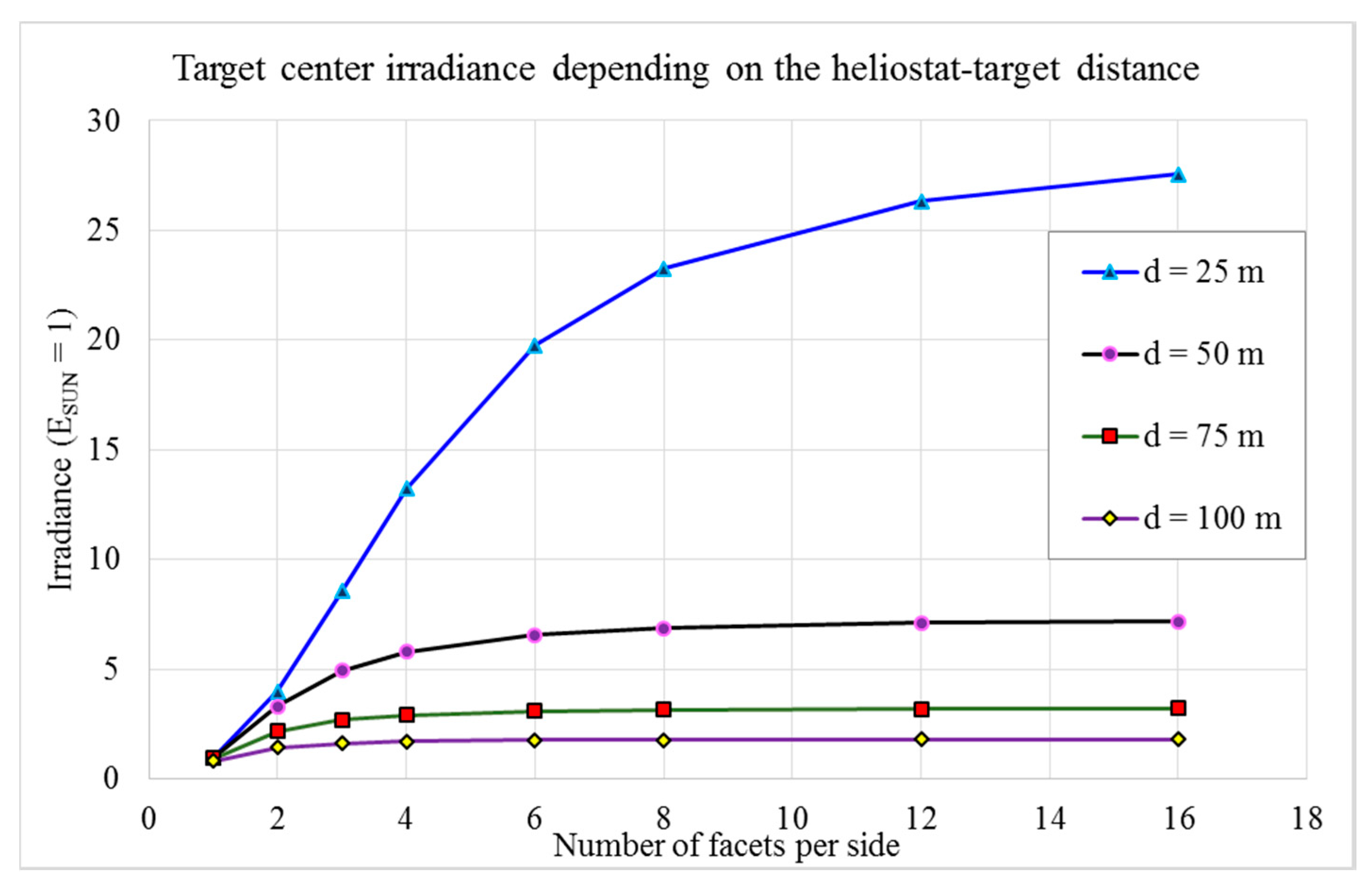
It is interesting to note that the concentration in x = 0 seems to have a maximum. This is confirmed by Figure 8, which shows the irradiance in the target center, at x = 0, depending on the values of the heliostat-target distance. In order to see how convenient could be to compose the heliostat surface with numerous facets, the irradiance is plotted versus the number of facets per side.

The result is quite intuitive: as far is the target from the heliostat, as useless is to divide the heliostat in many facets.

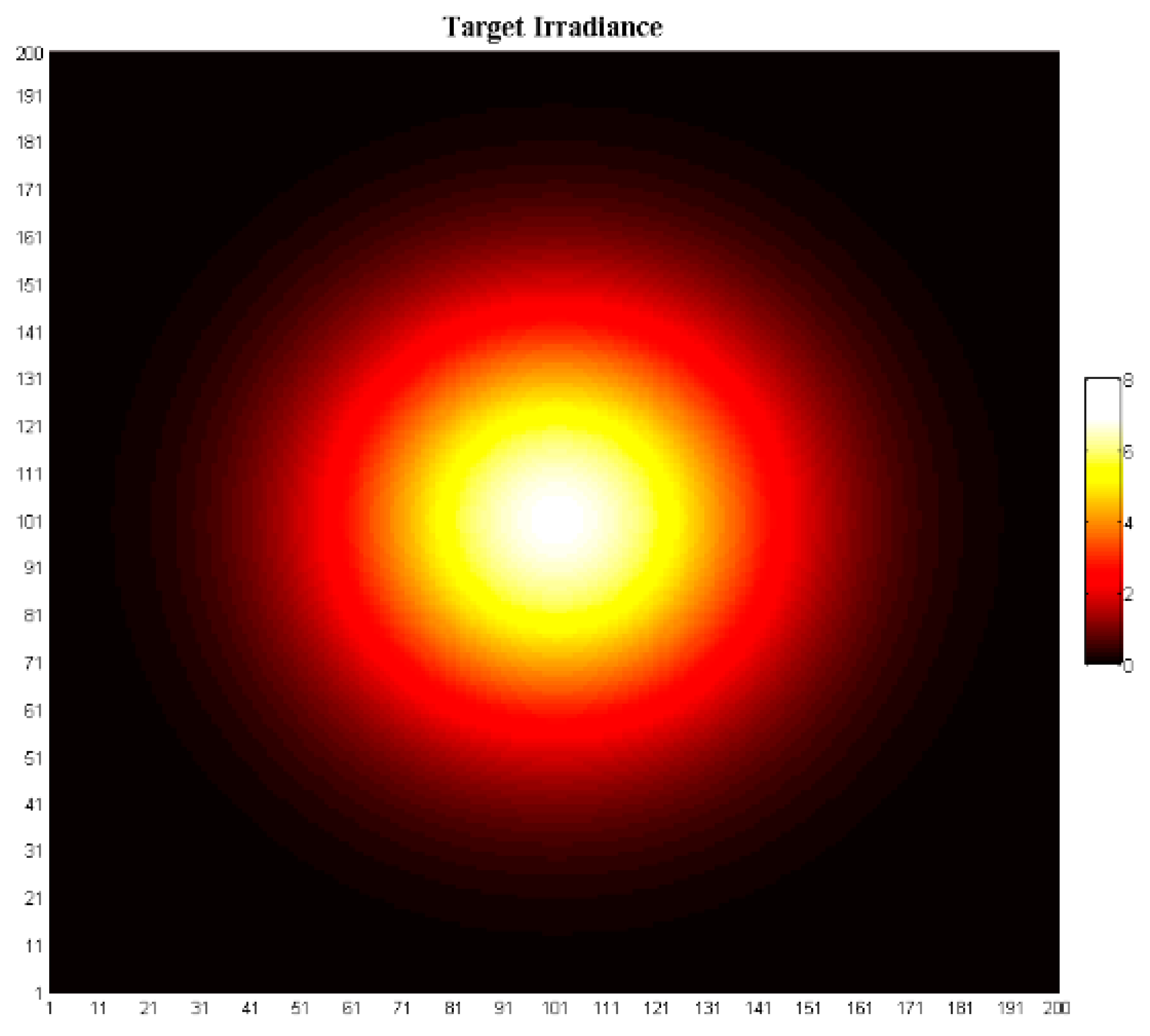
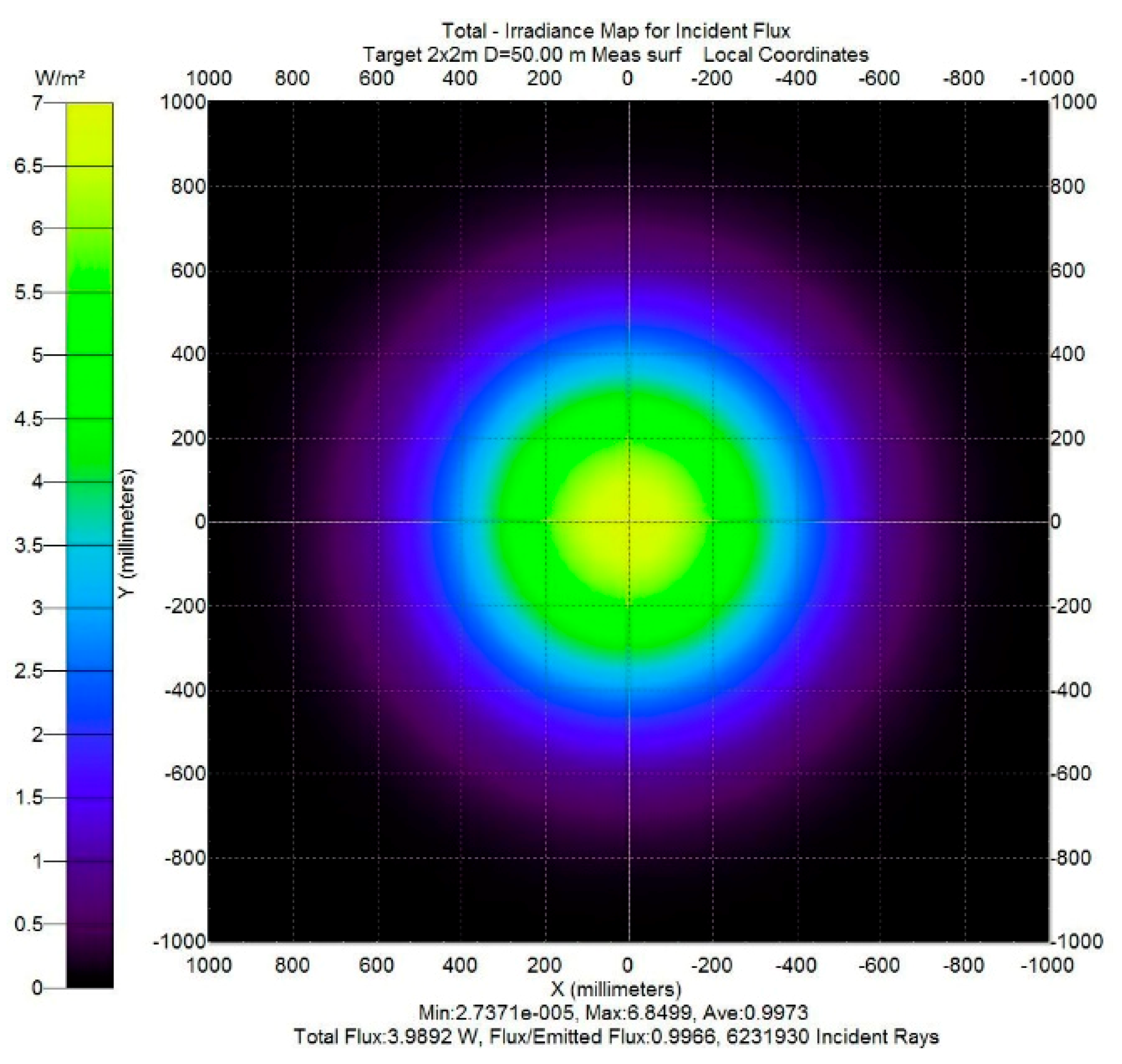
The map of the target is shown in Figure 9 for heliostat size 2 × 2 m (2L_F = 2 m) with 8 × 8 facets, target size 2 × 2 m, and heliostat-target distance d = 50 m. The result is expressed as concentration (with respect to the solar irradiance on the heliostat = 1). For comparison, in Figure 10 there is the result obtained from the simulation for the same configuration.

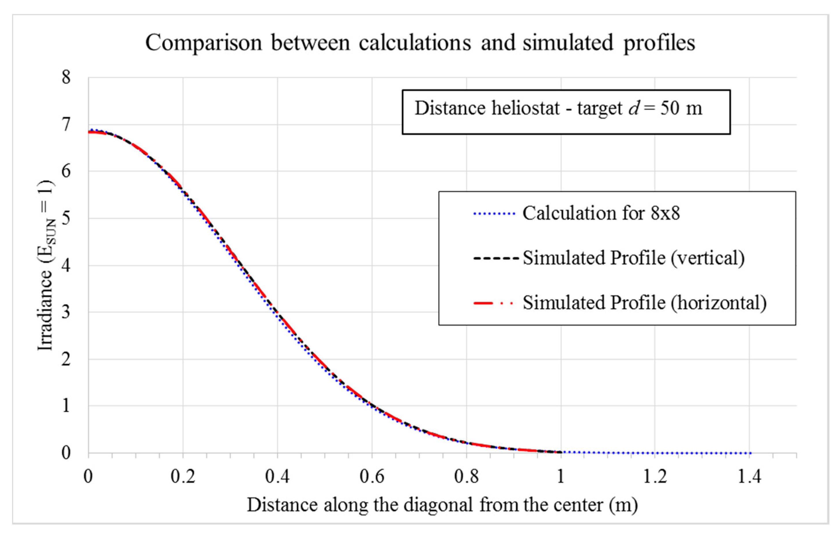
All the results obtained from the TracePro simulations are in accordance with the theoretical calculation. Figure 11 reports the comparison between the calculated profile and the two profiles of the simulated irradiance map. The calculated profile is diagonal on the target and the two simulated profiles (horizontal and vertical on the target) are diagonals with respect to the heliostat.

Considering the data of Figure 8 and the related calculation methods, it is possible to estimate that for the heliostat-target distance of 50 m the limit concentration on the target center, when the facets number → ∞ (i.e., L_F → 0), is 7.313. This result coincides with the maximum concentration value obtained by means of a simulation with a parabolic mirror (the limit for a faceted mirror when L_F → 0): the averaged concentration on a target of 20 × 20 mm is 7.316. The software utilizes a Monte Carlo method to generate the ray tracing, then the accordance with the previous result is very good.

Another additional confirmation of this result derives from the Lagrange invariant (for paraxial configuration, see [32] (pp. 18–19)). Since only the rays with direction near the central axis of the solar beam can be concentrated in the center of the target, the size of this zone can be calculated starting from the divergence with respect to the central axis of the solar beam. Considering a divergence of 0.01913 × σ (the Gaussian std. dev.), the related solid angle is 4.0 × 10⁻⁸ sr. The product of this value by the area of the mirror (4 m²) must be equal to the product of the angle subtended by the target toward the mirror area (0.001599 sr) multiplied by the area of the target central zone. Consequently the central zone of the target has an area of 1.0 × 10⁻⁴ m². Then, the part of the solar beam that has divergence less than or equal to 0.01 × σ is evaluated and the irradiation on the central zone of the target is calculated: the final result is a concentration value of 7.312, very near to the previous value. The difference between the value calculated by means of the integral on the target (7.313) and the theoretical value evaluated by the Lagrange invariance (7.312) depends on some very little approximations in the integral calculation, e.g., the modifications of the irradiance values due to the facet angles are not considered.

Considering Equation (4), it is easy to realize that in the point (x, y) = (0, 0) the irradiance value depends only on the ratio d/(2L_F) (because σ_XY ~ σ_θ·d, where σ_θ is constant). Thus, it is useful to evaluate the irradiance on the center of the target E(0, 0) in dependence of the facets number and of the ratio d/(2L_F), where d is the heliostat-target distance and 2L_F the side length of the squared heliostat. The results are shown in

Table 1. Irradiance on the center of the target (E_SUN = 1), where d is the heliostat-target distance and 2L_F is the length of the heliostat side; the limit is calculated by means of the Lagrange invariance.

Facets No. Per Side	Ratio d/2LF
	5	10	15	20	25	30	40	50	75	100
1	1.00	1.00	1.00	1.00	0.999	0.991	0.933	0.828	0.553	0.364
2	4.00	4.00	3.96	3.73	3.31	2.84	2.02	1.46	0.739	0.431
3	9.00	8.92	7.96	6.38	4.95	3.86	2.43	1.65	0.783	0.445
4	16.0	14.9	11.4	8.08	5.82	4.34	2.61	1.72	0.799	0.45
6	35.7	25.5	15.4	9.73	6.59	4.74	2.74	1.78	0.811	0.455
8	59.7	32.3	17.3	10.4	6.89	4.89	2.79	1.80	0.815	0.46
12	102	38.9	18.9	11.0	7.12	5.01	2.83	1.82	0.818	0.456
16	129	41.7	19.5	11.2	7.21	5.05	2.84	1.82	0.82	0.457
20	146	43.1	19.8	11.3	7.25	5.07	2.85	1.82	0.82	0.457
24	156	43.9	20.0	11.3	7.27	5.08	2.85	1.83	0.82	0.457
limit	181	45.6	20.3	11.4	7.31	5.10	2.86	1.83	0.821	0.457

; the last row is the limit value of concentration, evaluated by means of the Lagrange invariance.

4. Mirror Field

As example a field of mirrors with five rows and five columns (with row distance = 4 m and column distance variable) and a receiver at 20 m height can be considered. The horizontal distance between the central heliostat (3rd row/3rd column) and the target projection on the ground is 20 m, the std. dev. = 5.9 mrad; moreover, the target is inclined toward the central heliostat. For the sake of simplicity, the sun elevation is 45 deg and the azimuth is 0 (it corresponds to noon, because the field is located north of the tower). The calculation takes into account the cosine factor due to the inclination of the beams with respect to the heliostats other that the central one.

The data were obtained by means of a simple VBA procedure in an Excel datasheet, considering the x-direction and y-direction behaviors of the target irradiance for a set of single heliostats with side 2 m (L_F = 1 m). The calculation was repeated for another set of 25-faceted mirror heliostats with the same size but with different distance between the columns. Figure 12 shows the behavior for column distance 3 m, Figure 13 for column distance 10 m.

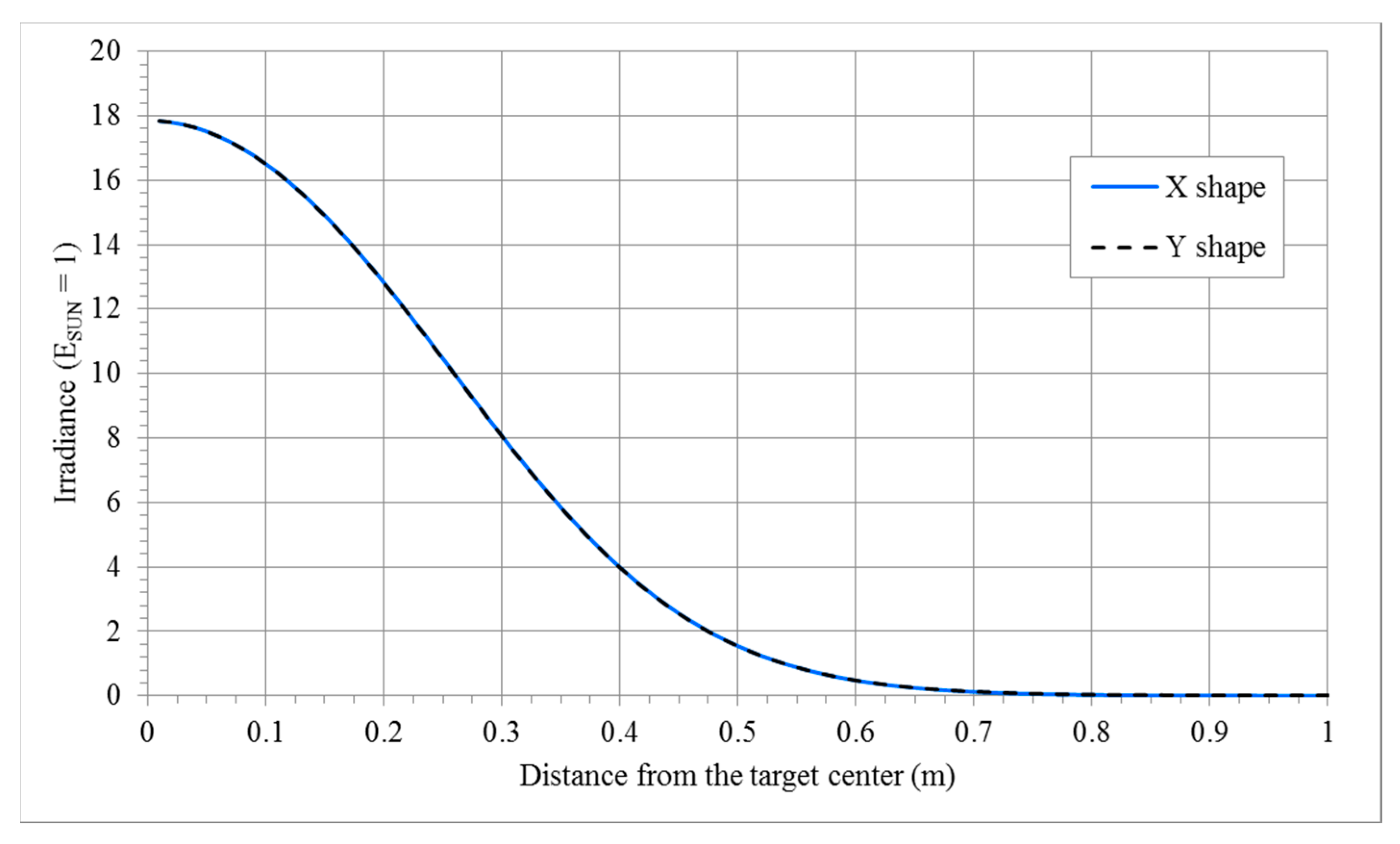
For the configuration of Figure 12 the spot is a circle (the behavior in x and y direction is the same, then only the y curve is represented on the graph), while in the case of Figure 13 the different behavior in the x direction with respect to the y direction becomes clear and the spot shape becomes an oval.

The same behavior is obtained for the simulated field: for comparison, Figure 14 displays the results obtained from TracePro with the parameters of Figure 13. The values are averaged over four raytracings, using 2.5 × 10⁸ rays per raytracing; each raytracing, based on the MonteCarlo method, starts with a different random seed. The central profiles of the simulated irradiance map are compared with the calculated profiles in Figure 15.

As shown, the accordance between TracePro simulation and calculated spot shape (in x and y directions) is very good, the difference between calculated and simulated profile is less than 2.5% up to 0.25 m from the target center and less than 5% up to 0.5 m from the target center. The reported difference is similar to the variation among the results of the four raytracings with different random seeds. Therefore, the proposed method is applicable for the evaluation of the entire heliostat fields too.

5. Discussion

The analysis, founded on the TracePro simulation, presents some results that have to be pointed out. Concerning the method, basically it is a simplified convolution analysis that does not take into account blocking and shadowing effects, but allows to obtain results in good accordance with the simulations. In particular, it should be noted that there are not many studies on flat heliostats, due to the fact that the most important analysis software (as HFLCAL for example) manages focusing mirrors. 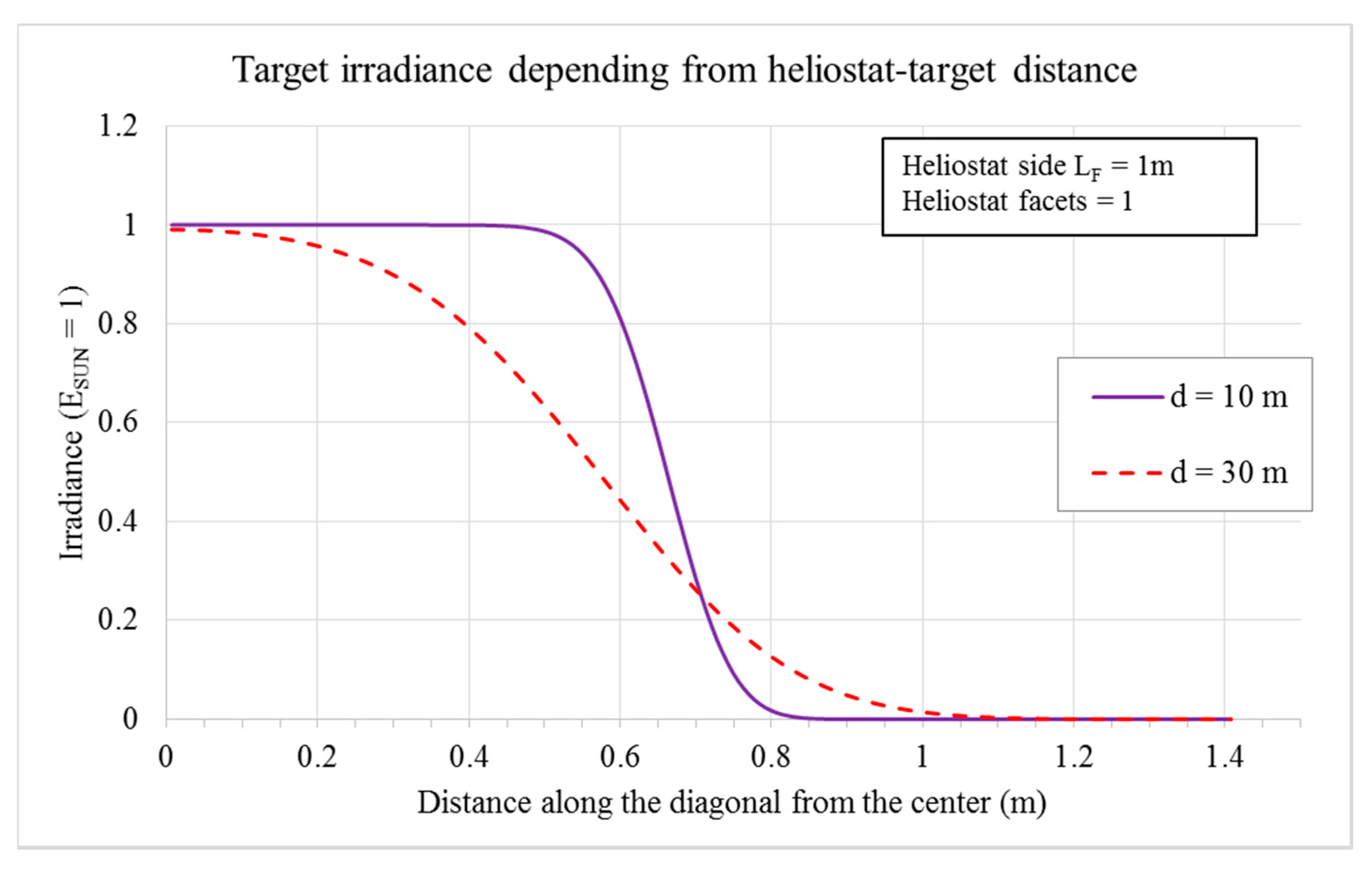An example of study about the flat heliostats is [12], where Elsayed et al. presented experimental results (for a laboratory set-up); in the conclusion, they noticed that the range over which the irradiance is constant is reduced when the mirror is moved further away from the receiver or the mirror size decreases (point 4, page 409). In the present work, the same conclusion derives from a confrontation of Figure 3 and Figure 4 and from the following Figure 16, which reports the irradiance variation on the spot for two different distances from the target. Figure 16 plots simulated irradiance profiles for single-facet heliostats with side 2L_F = 1 m at distance 10 m and 30 m.

Clearly, in Figure 16 the maximum irradiance value on the target is E_SUN (the heliostat is not focusing); this value can be increased if the heliostat is faceted, but the concentration has a maximum that depends on the heliostat-target distance (Figure 8). The issue was examined by Landman et al. in [33]: for canted flat facets, they define the image dimension as the sum of the projected size of the single facet and a term that takes into account the solar enlargement (Equation (3) page 129); correctly, the cited Equation shows that the image dimension has a minimum when the facet size tends to zero (it is the solar enlargement by the distance). However, due to the fact that there is the contribution of a single facet only, it is not immediately apparent that superimposing the spots from many facets there is a limit to the center irradiance on the target. In the present work it is shown that the concentration maximum is related, in addition to the presence of aberrations (for faceted heliostats that corresponds to an approximate canting), to a theoretical limit, as demonstrated by means of the Lagrange invariant in Section 3. The fact that with a faceted heliostat it is possible to reach an irradiance value on the center of the receiver similar to the irradiance generated by a parabolic heliostat is highlighted also by Riveros-Rosas et al. in [34], where a specific layout of a solar furnace is studied.

Surely, the method and results presented in this work constitute a rough evaluation of the irradiance on the target, because neither the blocking and shadowing effects, nor the asymmetry of the reflection beam from the heliostat are taken into consideration. Moreover, the canting was considered always perfect, that is economically plausible only for special applications (as some furnaces or scientific devices). Theoretically, it is possible also to modify the software in order to take into account imperfect canting, atmospheric absorption and blocking or shadowing, but it would constitute a significant complication (in particular concerning the last two phenomena), undermining the aim of this study. Nevertheless, in the early design phase it is important to have a fast evaluation of the best heliostat facet size both for structural and economic considerations; this is the scenario where the present work is applicable.

6. Conclusions

The aim of the present study is to supply methods, important parameters and results concerning the power density distribution of the spot generated on the receiver from a flat heliostat or a flat heliostats array. These methods and data are particularly useful in the design phase of a solar field to guide the optical designer in the development of the field configuration.

The layout with a flat heliostat, or a flat heliostats array, is very often utilized in CSP (Concentration Solar Power) plants with central tower. This mirror configuration can be associated, as a first approximation, to a Gaussian beam enlargement, which emerges as the convolution of the solar beam and the pointing errors due to components and assembly tolerances. It permits to elaborate a suitable function that describes the variation of the irradiance on the target.

In this work, the variation of the spot depending on the heliostat size or the facets size of a faceted heliostat is evaluated by means of both the numerical integration of that function and a non-sequential raytracing software, Lambda Research TracePro. The effect of various parameters are analyzed: side of the facets (2L_F from 0.5 m to 4 m), heliostat-target distance (d from 25 to 100 m), facets number (from 1 × 1 to 16 × 16). A test of the method on an array of heliostats demonstrates its applicability for a rough evaluation of the performance of a solar plant too.

The results obtained from the numerical integration are in good agreement with the corresponding TracePro simulations. The validity of the method is confirmed by an application of the Lagrange invariant to the Gaussian beam.

An example of the utility of this analysis is represented by Table 1, which synthesizes the concentration obtainable in a heliostat field changing the number of facets and varying the ratio between the heliostat-target distance and the facets side. The opportunity of having such an overview of the performance (as irradiance on the target center) of numerous possible configurations for the faceted heliostat field can address the designer in the selection of the most suitable field for a specific application. In particular, these results allow estimating the utilization of flat mirrors instead of concentrating mirrors or the minimum useful faceted size for a faceted heliostat, depending on the heliostat-target distance. Moreover, it is important to remark that there is a lower limit of the mirror size depending on the distance from the receiver: under this value, there is no increase of the concentration on the target.

These results are readily available for the designer of a solar field when a fast analysis of the project is requested. The proposed method is applicable to flat heliostats, to faceted plane heliostats, and also to arrays of flat heliostats. The method can be easily modified to take into account the different positions of the sun and to more accurately describe the behavior of a faceted heliostat.