Impact of Risk Aversion on the Operation of Hydroelectric Reservoirs in the Presence of Renewable Energy Sources

Abstract
:1. Introduction
- The presented model is more general than the previous work [16] as it takes into account a more realistic representation of the generation system. Thus, instead of a very stylized representation of the hydro system and a single thermal generator, this model uses a more detailed representation of the reservoirs during the whole planning horizon and it includes multiple thermal plants that can belong to different agents. In addition, instead of using utility functions to model risk aversion, the model implements the conditional value at risk (CVaR) [19] due to its suitability to be embedded within optimization models.
- Regarding [17], the presented model does not require to build in advance the extreme points of the polyhedron that define the risk set of each agent, and it takes into account the net-head dependency. In addition, the implemented model in the example-case section is not just a two-stage scenario tree, but a multi-stage scenario tree with 12 time periods (months) that can be used to analyze the impact of the risk aversion on the annual evolution of the main variables.
- Finally, this paper shows how the market equilibrium solution changes for different risk aversion levels of the involved agents, and uses an example case to quantify those differences.
2. Benchmark Model: Centralized Stochastic Hydrothermal Coordination Model
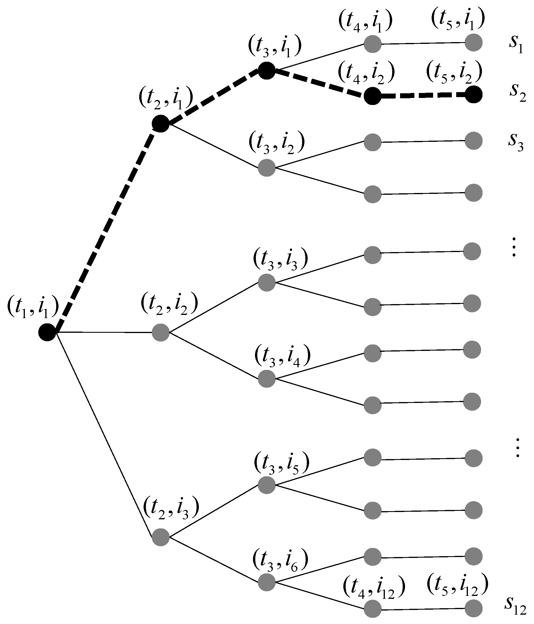
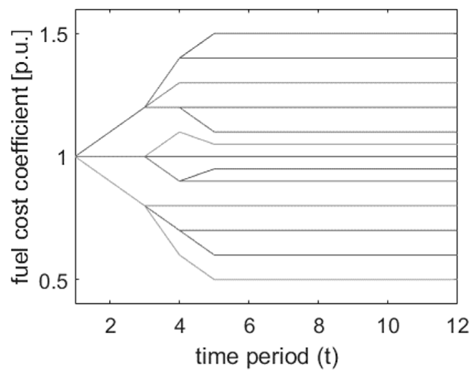
2.1. Modeling the Uncertainty Using a Stochastic Tree
2.2. Hydroelectric Generation
2.3. Mathematical Formulation of the Centralized Model
3. Market Equilibrium Model with Risk-Averse Agents
3.1. Market Equilibrium Concept with Risk Aversion Agents
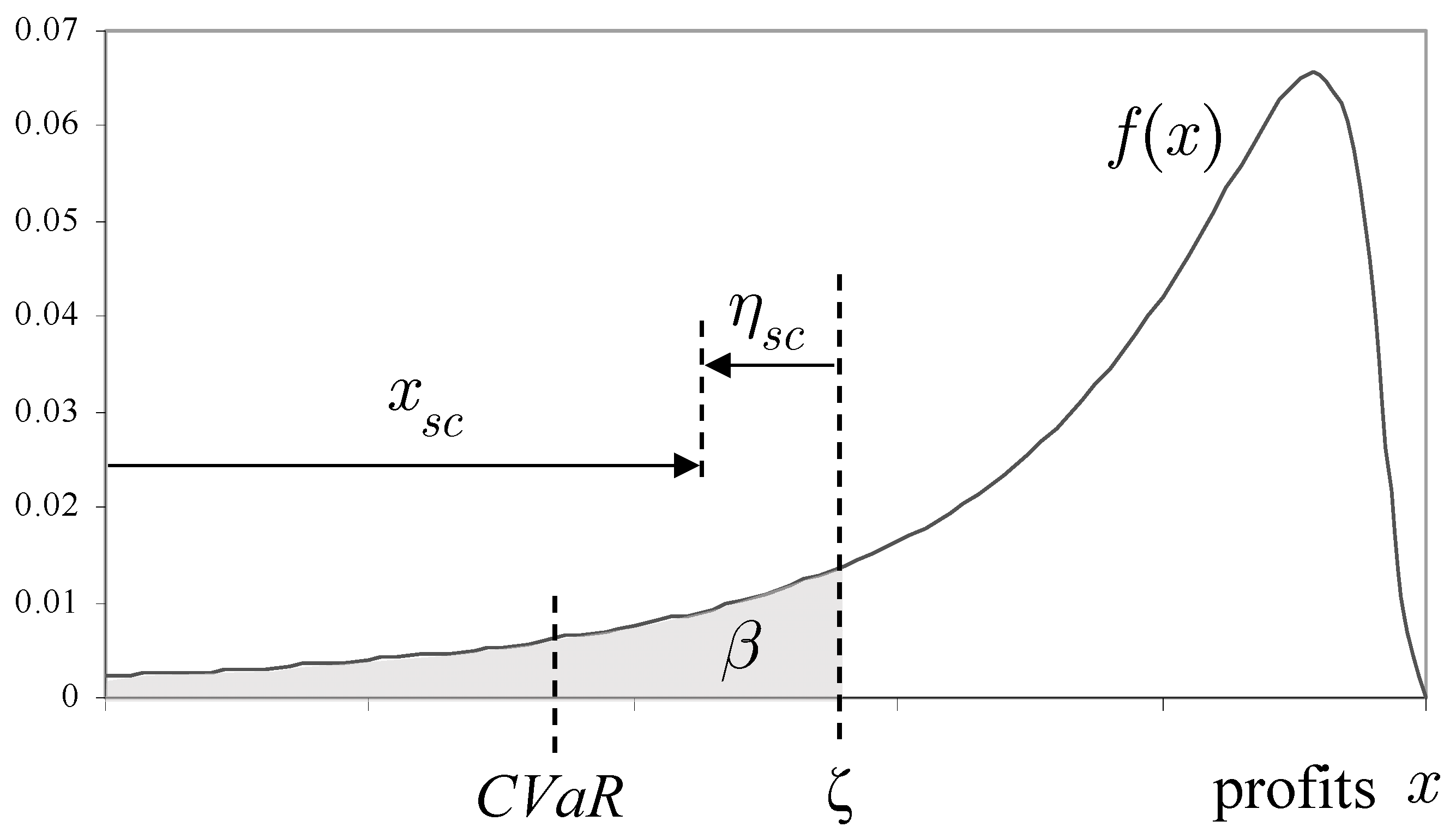
3.2. Modelling the Risk-Aversion with CVaR
3.3. Mathematical Formulation of the Market Equilibrium Model
4. Relationship between the Centralized and the Market Equilibrium Models
4.1. Optimality Conditions of the Centralized Model
4.2. Optimality Conditions of the Market Equilibrium Model
4.3. Impact of Risk Aversion Level
5. Results
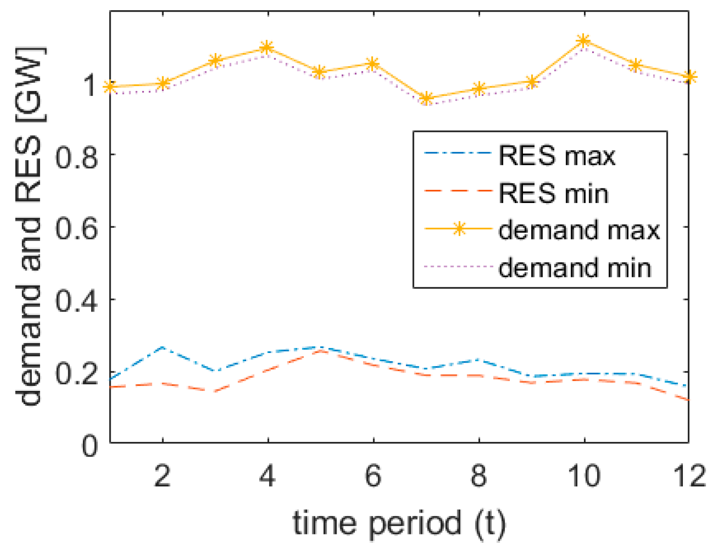
5.1. System Description
5.2. Numerical Solution of the Models
6. Discussion
7. Materials and Methods
8. Conclusions
Supplementary Materials
Author Contributions
Acknowledgments
Conflicts of Interest
Appendix A
- : Set of time periods
- : Set of hydro generators
- : Set of thermal generators
- : Set of renewable energy sources (RES) generators
- : Set of scenarios
- : Set of generation companies (market participants)
- : Set of all nodes of the multistage stochastic tree. Each node is identified and represented by : the time period (), and the node identifier within each time period ().
- : Set of terminal nodes
- : Set of all the nodes that are not terminal nodes, i.e.,
- : Set of all nodes included in scenario,
- : Subset of thermal generators that belong to generation company
- : Subset of hydro generators that belong to generation company
- : Father node of node in the multistage stochastic tree
- : Descendent nodes of node in the multistage stochastic tree
- : Set of all the scenarios that include the node in their path
- : Demand at node
- : Duration of the time that corresponds to node
- : Natural inflows at the reservoir of hydro generator in node
- : Probability of scenario
- : Probability of node
- : Power generation of renewable energy sources at node
- : Initial volume of water stored at the reservoir of hydro generator
- : Target volume of water at the end of the time horizon for hydro generator
- : Maximum reservoir capacity for hydro generator
- : Minimum reservoir capacity for hydro generator
- : Minimum water flow for hydro generator at node
- : Maximum water flow for hydro generator
- : Maximum output power of thermal generator
- : Confidence interval of each generation company
- : Risk aversion level of each generation company
- : Cost function of thermal generator , at node
- : Energy coefficient to translate water flow into output power of hydro unit
- : Profit obtained by generation company , in scenario
- : Volume of water stored in at the end of the time period of node
- : Flow of water released by the reservoir of hydro generator , in node
- : Water spillage of hydro generator , in node
- : Output power generated by hydro generator , in node
- : Output power of thermal generator , in node
- : Spot price in node
- : Conditional value at risk of each generation company
- : Value at risk of each generation company
- : Auxiliary variable used for CVaR computation
References
- De Queiroz, A.R. Stochastic hydro-thermal scheduling optimization: An overview. Renew. Sustain. Energy Rev. 2016, 62, 382–395. [Google Scholar] [CrossRef]
- Pereira, M.V.F.; Pinto, L.M.V.G. Multi-stage stochastic optimization applied to energy planning. Math. Program. 1991, 52, 359–375. [Google Scholar] [CrossRef]
- Schweppe, F.C.; Caramanis, M.C.; Tabors, R.D.; Bohn, R.E. Spot Pricing of Electricity; Power Electronics and Power Systems; Springer: New York, NY, USA, 1988. [Google Scholar]
- Rubin, O.D.; Babcock, B.A. The impact of expansion of wind power capacity and pricing methods on the efficiency of deregulated electricity markets. Energy 2013, 59, 676–688. [Google Scholar] [CrossRef]
- Denton, M.; Palmer, A.; Masiello, R.; Skantze, P. Managing market risk in energy. IEEE Trans. Power Syst. 2003, 18, 494–502. [Google Scholar] [CrossRef]
- Conejo, A.J.; Nogales, F.J.; Arroyo, J.M.; Garcia-Bertrand, R. Risk-constrained self-scheduling of a thermal power producer. IEEE Trans. Power Syst. 2004, 19, 1569–1574. [Google Scholar] [CrossRef]
- García-González, J.; Parrilla, E.; Mateo, A. Risk-averse profit-based optimal scheduling of a hydro-chain in the day-ahead electricity market. Eur. J. Oper. Res. 2007, 181, 1354–1369. [Google Scholar] [CrossRef]
- Sheikhahmadi, P.; Mafakheri, R.; Bahramara, S.; Damavandi, M.Y.; Catalão, J.P.S. Risk-Based Two-Stage Stochastic Optimization Problem of Micro-Grid Operation with Renewables and Incentive-Based Demand Response Programs. Energies 2018, 11, 610. [Google Scholar] [CrossRef]
- Fleten, S.-E.; Ziemba, W.T.; Wallace, S.W. Hedging electricity portfolios via stochastic programming. In Decision Making under Uncertainty: Energy and Power 128 of IMA Volumes on Mathematics and Its Applications; Greengard, C., Ruszczynski, A., Eds.; Springer: New York, NY, USA, 2002; pp. 71–93. [Google Scholar]
- Cabero, J.; Baillo, A.; Cerisola, S.; Ventosa, M.; Garcia-Alcalde, A.; Peran, F.; Relano, G. A Medium-Term Integrated Risk Management Model for a Hydrothermal Generation Company. IEEE Trans. Power Syst. 2005, 20, 1379–1388. [Google Scholar] [CrossRef]
- Karavas, C.-S.; Arvanitis, K.; Papadakis, G. A Game Theory Approach to Multi-Agent Decentralized Energy Management of Autonomous Polygeneration Microgrids. Energies 2017, 10, 1756. [Google Scholar] [CrossRef]
- Baringo, L.; Conejo, A.J. Risk-Constrained Multi-Stage Wind Power Investment. IEEE Trans. Power Syst. 2013, 28, 401–411. [Google Scholar] [CrossRef]
- Abada, I.; de Maere d’Aertrycke, G.; Smeers, Y. On the multiplicity of solutions in generation capacity investment models with incomplete markets: A risk-averse stochastic equilibrium approach. Math. Program. 2017, 165, 5–69. [Google Scholar] [CrossRef]
- Heidarizadeh, M.; Shivaie, M.; Ahmadian, M.; Ameli, M.T. A risk-based optimal self-scheduling of cascaded hydro power plants in joint energy and reserve electricity markets. In Proceedings of the 2016 6th Conference on Thermal Power Plants (CTPP), Tehran, Iran, 19–20 January 2016; pp. 76–82. [Google Scholar]
- Moghaddam, I.G.; Nick, M.; Fallahi, F.; Sanei, M.; Mortazavi, S. Risk-averse profit-based optimal operation strategy of a combined wind farm-cascade hydro system in an electricity market. Renew. Energy 2013, 55, 252–259. [Google Scholar] [CrossRef]
- Rodilla, P.; García-González, J.; Baíllo, Á.; Cerisola, S.; Batlle, C. Hydro resource management, risk aversion and equilibrium in an incomplete electricity market setting. Energy Econ. 2015, 51, 365–382. [Google Scholar] [CrossRef]
- Philpott, A.; Ferris, M.; Wets, R. Equilibrium, uncertainty and risk in hydro-thermal electricity systems. Math. Program. 2016, 157, 483–513. [Google Scholar] [CrossRef]
- Gérard, H.; Leclère, V.; Philpott, A. On risk averse competitive equilibrium. Oper. Res. Lett. 2018, 46, 19–26. [Google Scholar] [CrossRef]
- Rockafellar, R.T.; Uryasev, S. Optimization of Conditional Value-at-Risk. J. Risk 2000, 2, 21–41. [Google Scholar] [CrossRef]
- Birge, J.R.; Louveaux, F. Introduction to Stochastic Programming; Springer Science & Business Media: New York, NY, USA, 1997. [Google Scholar]
- Wood, A.J.; Wollenberg, B.F. Power Generation, Operation and Control; Jonh Wiley & Sons: New York, NY, USA, 1984. [Google Scholar]
- Conejo, A.J.; Arroyo, J.M.; Contreras, J.; Villamor, F.A. Self-scheduling of a hydro producer in a pool-based electricity market. IEEE Trans. Power Syst. 2002, 17, 1265–1272. [Google Scholar] [CrossRef]
- Ventosa, M.; Baillo, A.; Ramos, A.; Rivier, M. Electricity market modeling trends. Energy Policy 2005, 33, 897–913. [Google Scholar] [CrossRef]
- Ferris, M.C.; Dirkse, S.P.; Jagla, J.-H.; Meeraus, A. An extended mathematical programming framework. Comput. Chem. Eng. 2009, 33, 1973–1982. [Google Scholar] [CrossRef]
- Jovanović, N.; García-González, J.; Barquín, J.; Cerisola, S. Electricity market short-term risk management via risk-adjusted probability measures. IET Gener. Transm. Distrib. 2017, 11, 2599–2607. [Google Scholar] [CrossRef]
- Jing, L.; Xian, W.; Shaohua, Z. Equilibrium Simulation of Power Market with Wind Power Based on CVaR Approach. In System Simulation and Scientific Computing; Xiao, T., Zhang, L., Ma, S., Eds.; Communications in Computer and Information Science; Springer: Berlin/Heidelberg, Germany, 2012; pp. 64–73. [Google Scholar]
- GAMS Home Page. Available online: https://www.gams.com/ (accessed on 14 March 2016).
- Red Eléctrica de España. Available online: http://ree.es/en (accessed on 2 March 2018).


| Thermal Units | (GW) | (k€/(GW·h)) | (k€/(GW2·h)) |
|---|---|---|---|
| J1 | 0.2 | 30 | 30 |
| J2 | 0.5 | 45 | 15 |
| J3 | 0.2 | 35 | 30 |
| J4 | 0.5 | 40 | 15 |
| Hydro Units | (m3/s) | (hm3) | (hm3) | (hm3) | (MW/m3/s) | (MW/m3/s) |
|---|---|---|---|---|---|---|
| H1 | 400 | 1000 | 500 | 4000 | 1.3 | 1.00 |
| H2 | 200 | 800 | 400 | 3000 | 1.56 | 1.20 |
| t1 | t2 | t3 | t4 | ||||
|---|---|---|---|---|---|---|---|
| 0% | 0% | ||||||
| −15.31% | 0% | −6.34% | 0% | 0% | 0% | ||
| 0% | 0% | ||||||
| 0% | 0.61% | ||||||
| −26.23% | 0% | −16.60% | 0% | −8.44% | 0.64% | 0% | 0% |
| 0% | 0% | ||||||
| −18.72% | 0% | ||||||
| −39.57% | −12.72% | −56.14% | −24.94% | −23.58% | 0% | ||
| −20.34% | 0% | ||||||
| Model | Genco1 | Genco2 | ||
|---|---|---|---|---|
| (k€) | (k€) | (k€) | (k€) | |
| RN | 99,148.51 | 56,208.25 (*) | 103,892.21 | 58,705.98 |
| RA | 99,025.92 | 56,355.53 | 103,974.62 | 58,755.82 |
| \ | 0 | 0.2 | 0.4 | 0.6 | 0.8 | 1 |
|---|---|---|---|---|---|---|
| 0 | 0% | −0.021% | −0.031% | −0.036% | −0.039% | −0.041% |
| 0.2 | 0.125% | 0.106% | 0.099% | 0.095% | 0.093% | 0.092% |
| 0.4 | 0.168% | 0.152% | 0.146% | 0.143% | 0.141% | 0.140% |
| 0.6 | 0.203% | 0.188% | 0.182% | 0.179% | 0.179% | 0.179% |
| 0.8 | 0.223% | 0.208% | 0.202% | 0.202% | 0.203% | 0.202% |
| 1 | 0.291% | 0.275% | 0.268% | 0.264% | 0.262% | 0.262% |
| \ | 0 | 0.2 | 0.4 | 0.6 | 0.8 | 1 |
|---|---|---|---|---|---|---|
| 0 | 0% | 0.057% | 0.077% | 0.084% | 0.087% | 0.087% |
| 0.2 | −0.023% | 0.038% | 0.059% | 0.067% | 0.070% | 0.070% |
| 0.4 | −0.029% | 0.033% | 0.055% | 0.063% | 0.066% | 0.067% |
| 0.6 | −0.022% | 0.041% | 0.063% | 0.071% | 0.076% | 0.078% |
| 0.8 | −0.013% | 0.050% | 0.072% | 0.084% | 0.090% | 0.092% |
| 1 | −0.006% | 0.053% | 0.073% | 0.081% | 0.083% | 0.085% |
© 2018 by the authors. Licensee MDPI, Basel, Switzerland. This article is an open access article distributed under the terms and conditions of the Creative Commons Attribution (CC BY) license (http://creativecommons.org/licenses/by/4.0/).
Share and Cite
Jovanović, N.; García-González, J.; Cerisola, S.; Barquín, J. Impact of Risk Aversion on the Operation of Hydroelectric Reservoirs in the Presence of Renewable Energy Sources. Energies 2018, 11, 1389. https://doi.org/10.3390/en11061389
Jovanović N, García-González J, Cerisola S, Barquín J. Impact of Risk Aversion on the Operation of Hydroelectric Reservoirs in the Presence of Renewable Energy Sources. Energies. 2018; 11(6):1389. https://doi.org/10.3390/en11061389
Chicago/Turabian StyleJovanović, Nenad, Javier García-González, Santiago Cerisola, and Julián Barquín. 2018. "Impact of Risk Aversion on the Operation of Hydroelectric Reservoirs in the Presence of Renewable Energy Sources" Energies 11, no. 6: 1389. https://doi.org/10.3390/en11061389
APA StyleJovanović, N., García-González, J., Cerisola, S., & Barquín, J. (2018). Impact of Risk Aversion on the Operation of Hydroelectric Reservoirs in the Presence of Renewable Energy Sources. Energies, 11(6), 1389. https://doi.org/10.3390/en11061389