Abstract
The increasing share of renewable energy sources, such as wind and solar generation, has a direct impact on the planning and operation of power systems. In addition, the consideration of risk criteria within the decision support tools used by market participants (generation companies, energy services companies, and arbitrageurs) is becoming a common activity given the increasing level of uncertainties faced by them. As a consequence, the behavior of market participants is affected by their level of risk aversion, and the application of equilibrium-based models is a common technique used in order to simulate their behavior. This paper presents a multi-stage market equilibrium model of risk-averse agents in order to analyze up to what extent the operation of hydro reservoirs can be affected by the risk-averse profile of market participants in a context of renewable energy source penetration and fuel price volatility.
1. Introduction
Finding the optimal operation of the generators of a hydro-thermal system is a classic problem of the electric power industry that has deserved a lot of research in recent decades [1]. In particular, the uncertainty related to the hydro inflows has been one of the main concerns when planning the operation of hydroelectric reservoirs in the medium term (typically, one year). In this context, the application of multi-stage stochastic optimization techniques able to deal with the curse of dimensionality, such the stochastic dynamic dual programming (SDDP) [2], has been a common practice in many hydro-dominated systems such as Brazil, Norway, or New Zealand. In the context of a traditional vertical integrated system, the central planner (i.e., the System Operator) is in charge of obtaining such optimal operation with the aim of maximizing the expected social welfare.
The pioneering deregulation process that took place in Chile in the 80s paved the way for the posterior liberalization of the electric power industry in many countries during the 90s and later. The implementation of electricity markets based on marginal pricing principles [3] changed the way in which hydro and thermal generators were scheduled. Therefore, the centralized optimization approach was substituted in many systems by a market mechanism where the Market Operator (MO) is in charge of clearing the short-term spot market (typically a day-ahead auction complemented with real-time and balancing markets). In this context, generation companies (Gencos) are responsible for planning the optimal operation of their own assets, and for submitting the right offers to the MO that allow them to put into practice such optimal operation. In addition, the increasing level of intermittent renewable energy sources (RES), such as wind and solar, represents an additional challenge from the operation point of view [4]. Therefore, risk management has received a lot of attention in the electric power industry in order to help market participants to hedge their sources of risk for different time scopes [5]: short term ([6,7,8]), medium-term ([9,10,11]), and long term ([12,13]). Notably, the challenges of uncertain water inflows and the hydro distribution planning of cascade reservoirs in the new energy mix are addressed in the literature ([14,15]). However, in the liberalized market, risk-averse behavior of agents can have a big influence on the decision making process [16,17,18].
It is well-known that a perfectly competitive market results in the same operation as the theoretical social-welfare optimum. However, even in the absence of strategic behavior, the possible risk-aversion of market participants can lead to a different solution. Therefore, the fact that risk-aversion can lead to a market inefficiency is of paramount importance. In [16,17] it is proved that in a complete market where agents can trade risk products (for instance in the forward market), it is possible to achieve the same operation as central planning. However, the assumption of market completeness might not be realistic, and therefore it is necessary to assess the impact of risk aversion on the operation of the system in order to guide regulators to design additional mechanisms (such as demand procurement contracts), or to help market participants to understand the equilibrium solution for incomplete markets.
This paper presents a market equilibrium model where the players are Gencos that own typical generation portfolios, (coal plants, combined cycle gas turbines (CCGT), hydro units, and RES), and compete to supply the demand in the medium term taking into account that they can be endowed with different attitudes toward risk. The model is formulated as a multi-stage stochastic equilibrium problem. The major contributions of this paper can be summarized as follows:
- The presented model is more general than the previous work [16] as it takes into account a more realistic representation of the generation system. Thus, instead of a very stylized representation of the hydro system and a single thermal generator, this model uses a more detailed representation of the reservoirs during the whole planning horizon and it includes multiple thermal plants that can belong to different agents. In addition, instead of using utility functions to model risk aversion, the model implements the conditional value at risk (CVaR) [19] due to its suitability to be embedded within optimization models.
- Regarding [17], the presented model does not require to build in advance the extreme points of the polyhedron that define the risk set of each agent, and it takes into account the net-head dependency. In addition, the implemented model in the example-case section is not just a two-stage scenario tree, but a multi-stage scenario tree with 12 time periods (months) that can be used to analyze the impact of the risk aversion on the annual evolution of the main variables.
- Finally, this paper shows how the market equilibrium solution changes for different risk aversion levels of the involved agents, and uses an example case to quantify those differences.
2. Benchmark Model: Centralized Stochastic Hydrothermal Coordination Model
This section presents the benchmark model against which the operation of the generation system in the presence of risk-averse agents will be compared. This model is formulated as a centralized hydrothermal coordination problem where the objective function is to minimize the expected operation cost subject to satisfy the demand, and to all the technical constraints of the generators. The existence of uncertain parameters makes it necessary to formulate a multi-stage stochastic problem as explained hereafter. The nomenclature used throughout the paper can be seen in the Appendix.
2.1. Modeling the Uncertainty Using a Stochastic Tree
Many of the parameters used to model the generation system can be considered as known input data such as the nominal technical characteristics of the generating units (maximum power, input-output curves, etc.) or the initial value of the hydraulic reserves. However, there are many other parameters which are subject to uncertainty. Among them, the ones linked to the meteorology are crucial. On the one hand, the amount of rain or snow affects the level of hydroelectric energy stored in the reservoirs. In fact, the possible scenarios of natural hydraulic inflows constitute one of the most significant concerns when planning the medium term operation of the system. Other examples are the wind speed that determines the power that can be produced in wind farms, or solar radiation conditions for electrical production in photovoltaic or thermo-solar installations. On the other hand, meteorological factors also affect the electricity demand, which also depends on the economic activity and working patterns. Finally, the fuel prices of conventional thermal generators play a key role when determining the optimal dispatch of the generators, and the fluctuations in the coal and natural gas markets are also important sources of uncertainty.
A common approach for taking into account this uncertainty within an optimization model is to adopt a discrete representation of the probability distribution of all the random parameters in the form of a multistage scenario tree that considers the non-anticipative criterion of the decisions, (see [20]). Figure 1 shows an example of a multistage scenario tree that consists of nodes.
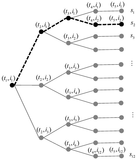
Figure 1.
Example of stochastic tree representation used to model the uncertainty.
Each one of the nodes is denoted by where is the time stage and is the position of the node at that time period. Given that every node as a single predecessor, it is common to use the term father node that is indicated by . For instance . In addition, the descendants of each node are denoted by . For example, .
Notice that the first node, i.e., the root node denoted as , is unique and it represents a here and now decision node as the value of the decision variables corresponding to it will be the same for all the scenarios. A typical example of this kind of decisions is the problem of determining the level of the reservoirs at the end of the first time-period knowing that the future natural inflows are uncertain. The posterior decision variables are recourse functions as they can be adapted as far as the uncertainty is being unveiled. All the branches can be characterized by a certain probability of occurrence, which leads to a total probability of occurrence of each scenario that satisfies that . Notice that each scenario is made of a whole set of nodes starting at the root node, and finishing in a terminal node, i.e., a node without any descendant. The set of nodes that belong to a given scenario are denoted as . For instance, the nodes that correspond to scenario have been highlighted in Figure 1. In addition, every node can also be characterized by a probability of occurrence denoted by .
2.2. Hydroelectric Generation
The power generated by a hydro unit depends on the water flow impacting the blades of the turbine and the net head, i.e., the difference between the elevation of the stored water and the elevation of the turbine drain, minus energy losses within the pipeline. In addition, the output power also depends on the efficiency of the turbine, the drive system and the generator. In order to model these relationships, it is common to use a family of input–output curves relating the water flow and the output power for each possible net-head value [21]. These input–output curves are very common in short-term hydro scheduling models [22], where the hourly generation of the hydro plants needs to be carefully modeled. However, in medium-term models it is usual to aggregate the production of many hours into a representative time period (for instance, all the peak hours of the working days of a given week). In this case, instead of the instantaneous relationship between power and flow rate, it is more relevant to model the ratio between the energy produced during such aggregated time-periods and the total volume of water released through the hydro turbine. This ratio is named as the energy coefficient, and for a given hydro plant , it is denoted by . Instead of assuming a static representation (as in [17]), this paper considers its dependency on the stored volume of water given that the net head changes with respect to the volume of water stored accordingly to the shape of the pond.
2.3. Mathematical Formulation of the Centralized Model
The objective of a centralized planner is to find the operation of the system that minimizes the expected cost while satisfying the demand balance equation and all the technical constraints of the system. The objective function can be formulated as
Notice that in (1), the costs of the thermal generators at each node are multiplied by the probability and the duration of the corresponding node. In addition, the per-hour cost functions of each generator depend on the power produced by them , and they can be different for each node in order to allow different fuel-price scenarios.
The optimization problem is subject to the following set of constraints:
Equation (2) establishes that the sum of the production of all the thermal generators () plus the sum of all hydroelectric units () plus the generation of renewable energy sources () must satisfy the demand at every node. Notice that for each constraint, its corresponding Lagrange multiplier is shown after the symbol that indicates complementarity. The Lagrange multiplier of (2) is represented by and it measures what would be the impact on the objective function if the demand in this particular node increases by one unit.
Equation (3) establishes the water balance equation: the volume of stored water at the reservoir of hydro unit at the end of the time stage that corresponds to the node is equal to the volume of water at the end of the previous period defined by the father node, , plus the amount of water that corresponds to the natural inflows , minus the amount of water due to the water flow released to generate hydro power, , minus the possible spillages, . In the particular case of the root-node, the volume of the father node is the initial volume, , which is input data. In addition, for the particular case of the terminal nodes, , the volume stored will not be a variable of the problem but the predefined target value at the end of the planning horizon, i.e., .
The relationship between the water flow discharged from the hydro turbine, , and the output power generated, , is expressed in (4) where is the energy coefficient that depends on the volume of water stored at the reservoir. The water flow limits of hydro units are established in (5) to model the physical limits of the intake of the turbine or any other water right such as minimum ecological flows. Notice that the generation limits of the hydro units are a consequence of the joint consideration of Constraints (4) and (5). However, in case the electric generator had a more restrictive power limit, it would be possible to add a new constraint imposing such limit. The maximum and minimum limits for thermal generators are taken into account in (6). Notice that, for the sake of simplicity, the existence of minimum stable loads for thermal generators has not been considered as this would require the usage of binary variables. As the presented model is intended to illustrate the impact of risk aversion levels on the operation of the hydro reservoirs in the medium term, all the issues related to a detailed modelling of thermal generators and their intertemporal constraints (such as ramps), have been neglected. The limits of the reservoirs are included in (7) which are formulated for all the nodes of the tree except for the terminal nodes, given that as it was mentioned before, at the last stage the volumes are fixed to the target level which is supposed to be feasible without any loss of generality. Finally, the non-negativity constraint of spillages is formulated in (8).
3. Market Equilibrium Model with Risk-Averse Agents
3.1. Market Equilibrium Concept with Risk Aversion Agents
One of the consequences of the deregulation of the electric power industry in the late 90s and the implementation of wholesale electricity markets in many countries around the world is that traditional operation and planning models had to be adapted to represent the competition of market participants. Among the variety of possible techniques, equilibrium models emerged as a solid framework to model the new situation [23]. The basic idea is to find the Nash Equilibrium (NE) of rational agents that are competing in a market where their payoff functions are interdependent. Let be the utility function of market participant that depends on its own strategies, , and on the ones of its competitors, . The NE solution satisfies that no one is incentivized to deviate unilaterally from that solution, i.e., , where it is taken into account that the selected strategies must belong to the set of feasible ones, . This is equivalent to formulate the simultaneous maximization of the utility functions of all the market participants, taking into account the interdependency of their actions. Therefore, the NE has the form of MOPEC (multiple optimization problems with equilibrium constraints). In the case of a set of generation companies that compete to supply the demand, the NE could be formulated as
where represents the spot market clearing where quantities are traded at price (see [24]).
In an electricity market it is common to assume that the utility function of generation companies is the obtained profit, i.e., the difference between market incomes and the generation costs. However, given the inherent uncertainties of the power system, it is necessary to define such utility taking into account that market profits depend on a stochastic process. Let us assume that all market participants share the same information about such stochastic process, where is the probability distribution that is common knowledge. Let be a vector whose components are the profits obtained by agent for all the finite scenarios used in the stochastic tree representation. One possible way to define the utility function of the market participant is to compute the expected value of the obtained profits, . However, for a risk-averse agent, it is possible to define its utility in terms of a coherent risk measure such as the conditional value at risk () [19] that will be reviewed in the next subsection. The linear combination of the expected profit and the is also a coherent risk measure, and therefore the objective function of a risk averse agent can be defined in general terms as
Notice that in (10), the parameter satisfies and it represents the risk-aversion level of the agent. The particular case of is equivalent to the risk-neutral setting. In the following section, we will analyze how the market equilibrium solution changes with respect to the values of .
3.2. Modelling the Risk-Aversion with CVaR
Conditional value at risk () is a coherent risk-measure that has been applied to model the risk-aversion of electricity market participants in many research works ([8,9,10,25,26]). In this paper, we follow the same approach proposed in [19] that allows computing of using a set of linear equations. Let be the value at risk at a confidence level of . This value represents the minimum profit that is achieved with a probability . As shown in Figure 2, represents the average value of the profits in the worst cases. Mathematically, it can be defined as

Figure 2.
Profits distribution, value at risk (), and conditional value at risk ().
The set of linear equations to model are detailed in the next section (Equations (20)–(22)). In that formulation, the positive auxiliary variable is defined as .
3.3. Mathematical Formulation of the Market Equilibrium Model
The market equilibrium solution can be obtained by formulating the simultaneous optimization of the utility function of all the market participants, subject to the market clearing constraints where sellers and buyers agree to trade electricity at a given price. According to what has been explained in Section 3.1, the market equilibrium can be formulated by Equations (12)–(22) (which are replicated for every agent) plus the market clearing formulated in (23):
For all agents
Subject to
Equation (12) establishes the objective function of each agent. Notice that in order to compute the expected profit, all the market participants share the same probability functions. Equation (13) defines the profit of market participant in scenario as the sum of the market incomes minus the generation costs (only thermal). Market incomes are computed by adding all the thermal, hydro, and RES generation that belong to such market agents, remunerated at the market price for all the nodes that comprise the scenario and taking into account the probability and the duration of each node. Equations (14)–(19) are analogous to the (3)–(8) as explained in Section 2.3, with the only difference that they are applied only to the generation units that belong to their corresponding market participant . Equations (20)–(22) are the set of linear constraints that allow to compute the where represents the value at risk for agent , and is an auxiliary variable to account only for the positive values of the difference between the and the profit of each scenario, .
The previous equations must be replicated for all market participants and complemented with the spot-market clearing where all the market participants participate selling the production of their thermal, hydro, and renewable generators at price :
4. Relationship between the Centralized and the Market Equilibrium Models
The objective of a centralized planner in charge of planning the operation of the electric power system is to maximize the total welfare of producers and consumers. For the case of an inelastic demand, this welfare maximization is equivalent to minimizing the total operational cost while satisfying the demand at every time stage as presented in Section 2.3. The idea that the same solution can be obtained by a market mechanism relies on Adam Smith’s “invisible hand” hypothesis that states that an efficient allocation of resources can be achieved by competitive markets, supported by the welfare theorems of microeconomics. In this sense, regulatory bodies in charge of designing the electricity market mechanisms aim to ensure that market functioning maximizes the total welfare of producers and consumers in the same manner as in an hypothetical perfect centralized planning. However, there are several reasons why market results can deviate from the theoretical social optimum. The most obvious one is the possible exercise of market power due to a strategic behavior of generation companies that might not reflect the true generation costs in their offers. However, even in the absence of such strategic behavior, the existence of uncertainty can lead also to a market inefficiency as demonstrated in [16,17]. In both works, it is proved that risk trading (for instance, by signing forward markets with risk-neutral agents such as the aggregated demand), can lead again to the optimum centralized solution even in case of risk-averse agents.
To study the possible equivalence between the centralized optimum planning and the market equilibrium in the context of the multi-stage stochastic framework presented previously, the Karush–Kuhn–Tucker (KKT) conditions for both settings are derived and compared hereafter.
4.1. Optimality Conditions of the Centralized Model
The first step to derive the KKT conditions of the centralized problem (1)–(8) is to build the Lagrangian function as shown in (24):
Equaling to zero the first derivative of the Lagrangian with respect to the primal variables allows us to write the first set of the KKT optimality conditions
The rest of KKT have been omitted for the sake of simplicity (equality constraints, inequality constraints, and slackness complementarity conditions).
A well-known result, which is in the core of the marginalist theory, is that in case the thermal generator is operating within its limits (i.e., , by (25) if follows that the dual variable of the demand balance constraint is the marginal cost of that generator (affected in this case by the duration and the probability due to the stochastic formulation with not-hourly time periods)
Another interesting remark is related to the interpretation of the Lagrange multiplier , that represents the marginal water value as it measures the savings in the objective function if one extra unit of natural inflows, , were available in that period. In case of a determinist formulation (a single scenario where every node has a single descendent), if the reservoir is being operated within its limits, i.e., , and if the net head effect could be neglected, i.e., , then the marginal water value in both time periods (the node and its descendent) would be the same.
4.2. Optimality Conditions of the Market Equilibrium Model
The Lagrangian function of the optimization problem solved by a particular agent, , Equations (12)–(22), is
The first order conditions for market participant , can be formulated as
4.3. Impact of Risk Aversion Level
This subsection analyses the impact on the equilibrium solution of the risk-aversion level of market participants.
To start with, let us assume that all market participants are risk-neutral. In this case, . By (38), it follows that , and by (39) it can be written that . As are non-negative multipliers, it follows that . In this case, Equation (37) can be rewritten as
The interpretation of (41) is that in the risk-neutral equilibrium, the Lagrange multipliers of the Equation (13), formulated for all the market participants for every scenario, must coincide with the probability of that scenario. Then, Equations (32) and (33) become
Given that the probability of one node can be computed as the sum of the probabilities of all the scenarios that cross that node in their paths from the root node until the terminal nodes, we can write
In addition, if we define the following relationship
then replication of Equation (32) for all the market participants leads to the same ones as the defined by (25). Applying the same idea to all the remaining equations, the same set of equations as the optimality conditions of the centralized problem would be obtained. Therefore, it can be concluded that the operation of the generation system that corresponds to the risk-neutral market equilibrium will be exactly the same one as in the centralized optimal operation.
However, in case there is at least one risk-averse agent, i.e., , then the operation of the system could differ from the centralized one given that (41) would not be satisfied. In this case, from (37) it follows that
The Lagrange multipliers can be interpreted as the risk-adjusted probabilities which are different for each agent. These risk-adjusted probabilities are the ones that market agents should assign to the scenarios so that the maximization of their expected profits according to them, would result in the same solution as the risk-averse operation. However, this interpretation requires a demonstration that satisfies the requirements of a probability measure. Given the non-negativity constraint of , Equation (45) forces to be positive. In addition, summing for all scenarios both sides of Equation (45), it results in the following expression
By (38) and (39), it follows that , and therefore it leads to the next result:
Once that it has been proven that can be interpreted as the risk-adjusted probabilities, it is interesting to provide some additional insights. Taking the Equations (38) and (40) into account, it follows that
Assume that the profit for a given scenario is strictly lower than the value at risk . Then Constraints (20) and (22) would be active and not-active respectively. Therefore, for that scenario, it would be satisfied that and . Then Equation (48) for this particular case would be
On the other hand, for a scenario where the profit exceeds it would be satisfied that . Then, by (45), we can derived
Both expressions cannot be computed ex-ante, unless a reasonable estimation of which scenarios give place to the worst profits is available.
Finally, for a given node, the risk-adjusted probabilities of each node can be computed as
5. Results
This section presents the obtained results of the centralized model (CEN), market equilibrium risk-neutral (RN) and the risk-averse model (RA). The main aim is to identify the impact of risk aversion on the operation of hydro reservoirs in the presence of renewable energy sources. Moreover, the mutual influence of agents’ different risk aversion levels on the results is also studied.
5.1. System Description
The power system presented in this case study is a scaled-down version of the Spanish mainland electricity market (see Section 7). In order to represent the uncertainty, a stochastic tree has been implemented where after period (the ‘here and now’ decision) there are 3 new nodes in , followed by 9 nodes in , and finally 27 nodes from to . Therefore, the uncertainty is modeled with 27 scenarios of the following input data: demand, RES, water inflow and the fuel cost. The time horizon is considered to be 12 months, where the first period () starts in October as in Spain the hydrological year goes from October until September. Each month has its corresponding duration () in hours depending on the number of days. In Figure 3, the maximum and minimum values of the RES and demand are presented per each time period. Notice that the highest share of the RES in the demand per month is 28% () and the lowest one is 12% ().
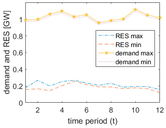
Figure 3.
Demand and renewable energy sources (RES) forecast.
Regarding the power generation, the system consists of four thermal units (see Table 1) and two hydro plants (see Table 2), which belong to two Gencos. The first agent Genco1 owns two thermal units ( and ), and the hydro unit . The second agent Genco2 owns the other two thermal units ( and ) and the second hydro unit . Both agents share a half capacity of the RES production and a half of the water inflow forecast. The thermal generation represents coal units ( and ) and CCGT ( and ). These thermal generators do not behave strategically, and their cost functions have been tuned to cover a representative range of real marginal costs. In particular, the cost function of a given thermal generator is a quadratic polynomial which results in a linear marginal cost function

Table 1.
Parameter data of thermal units.
Table 2.
Parameter data of hydro units.
For example, the marginal cost of the generator at its maximum production is 42 €/MWh. The factor fuel cost coefficient allows to increase or reduce the total cost by assigning different values to at each time period. Taking into account the uncertainty of the fuel prices in the time horizon of 12 months, different scenarios in Figure 4 represent the price volatility that agents can face. Notice that some of the 27 scenarios share the same values of and this is why in the figure one can only see 13 final leaves (each scenario considers a different combination of all the uncertain parameters that can be seen the detailed input data provided as Supplementary Materials).

Figure 4.
Fuel cost coefficient scenarios, .
Table 2 shows the parameter data of the hydro units. Note that the hydro unit has a maximum water flow two times larger than , and the hydro inflows are considered to be the same for hydro reservoirs. The uncertainty of the hydro inflows is modeled with 27 different scenarios and the maximum and the minimum ranges can be seen in Figure 5.
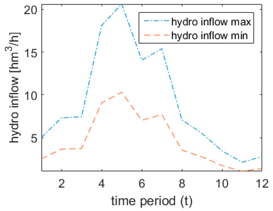
Figure 5.
Hydro inflow range.
The energy coefficient to translate water flow into output power of the hydro unit is expressed as
where it can be seen that when the volume of the reservoir is at the minimum level, the energy coefficient corresponds to the minimum one, , as the net head will be the lowest. When the reservoir is at its maximum capacity, the energy coefficient is the maximum one, . Any intermediate volume stored at the reservoir will result in the linear interpolation between those extreme values. It is important to notice that this representation allows to take into account that with the same amount of released water, the obtained energy (and therefore market incomes) can be different.
5.2. Numerical Solution of the Models
In this section, the following results are presented: comparison of the centralized and risk-averse models, the impact of risk aversion on the hydro reservoir operation, and finally the expected profit and the value of two market agents for different risk profiles.
As demonstrated in the Section 4.1, both CEN and RN models lead to the same optimal results: identical operation of the thermal units, identical operation of the hydro reservoirs, identical generation costs, identical prices taking into account Equation (25), etc. Given that the amount of output variables is too large to be presented here, Figure 6 shows two illustrative examples: the coverage of the demand through the whole year for the two scenarios with the more extreme inflows (Scenario 1 for high water inflows, and Scenario 27 for very low ones). It is noticeable how the system utilizes differently the available hydro energy, where, for example, the hydro reservoir of the has a level of 4000 hm3 in Scenario 1 and a level of 2543.356 hm3 in Scenario 27 at the end of the period . However, the operation for the time period is exactly the same due to the non-anticipative criterion at the first stage.
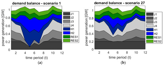
Figure 6.
Demand balance for Scenario 1 (a) and Scenario 27 (b) for the centralized case.
Another interesting result is related with the social welfare. Summing the expected profit of the two agents from the RN model (Genco1 99,148.51 k€ and Genco2 103,892.21 k€) and adding the total cost of the operation (190,141.82 k€) provide sthe same ‘demand payment’ that would be obtained in the CEN case if the marginal cost were used to charge the consumption (393,182.54 k€).
In order to decrease the risk of the uncertain parameters, the agents may deviate from the centralized hydro management planning. This is illustrated in Table 3 that shows the relative difference between the hydro reservoir levels () at the end of each time period for each Genco and assuming that both agents are pure risk averse agents ( for both).
Table 3.
Relative change of the hydro reservoir levels between the risk neutral and risk averse cases.
The following results emphasize the agents’ risk aversion influence on the hydro reservoir levels, particularly in the period when the RES decreases by 16% and the demand increases by 6% in average, compared to the period (see Figure 3). Figure 7 shows the relative difference between the average reservoir level in period for the RN and the RA case of the hydro reservoirs belonging to Genco1 (a) and Genco2 (b) for different risk-aversion levels.

Figure 7.
Hydro reservoir relative change in the period t3 for Genco1 (a) and Genco2 (b).
In the equilibrium based models, the risk aversion of the one agent affects the payoff outcome of the other agent. As an example, the case where both agents have extreme risk aversion () is compared with the risk neutral case in Table 4 that shows the expected profit and the value. Notice that Genco1 increases its value while the expected profit decreases. At the same time, Genco2 has a higher value and a higher expected profit.
Table 4.
Expected and values (μ1 = μ2 = 1).
Figure 8 shows the change of the value for both agents when they change their risk aversion from 0 to 1. The z-axis shows the relative change of the value in comparison to the RN case (). Although the changes in percentages have a low magnitude, in real terms the impact is not so negligible (for instance, a percentage of 0.05% corresponds, in this setting, to 30,000 €). Note that the Genco1 risk aversion has an interesting impact on the value of the Genco2 (see Figure 8b).
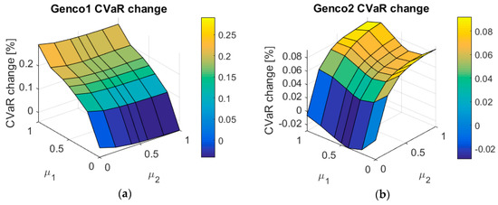
Figure 8.
value relative change for Genco1 (a) and Genco2 (b).
To better understand the impact of risk-averse agents in the equilibrium, the graphical data from Figure 8a,b are shown in Table 5 and Table 6, respectively.
Table 5.
Relative change of values for Genco1.
Table 6.
Relative change of values for Genco2.
6. Discussion
Given the previous results, it can be pointed out that in the equilibrium setting, risk-aversion can have a significant impact on the hydro reservoirs’ operation that can deviate from the centralized planning. As the objective of this paper is to study to what extent the risk-aversion affects such operation, results presented in Table 3 deserve some additional discussion. Notice that the relative change between the reservoir levels corresponding to the ideal centralized operation (which are the same ones as in the risk-neutral case), and the market equilibrium case where both agents are pure risk-averse players, take place since the first period. This is more relevant for the reservoir of unit which has the highest decrease in the third branch of the stochastic tree in . It is interesting to highlight that the operation of the first month for the reservoir of (which is a here and now decision), leaves the reservoir more empty (−26.23%) than in the centralized operation. The interpretation of this fact is clear: the Genco1 prefers to use the available water in the first month where the uncertainty of market prices is null in order to reduce the future risk of more volatile incomes in posterior months. Moreover, a similar analysis could be carried out to analyze the impact on the other here and now variables: the power generated by all the thermal and hydro units, and the water released or spilled by hydro plants in the first stage, .
Regarding the analysis of how the risk-aversion level of each agent affects the hydro operation, Figure 7 shows that higher risk aversion leads to a higher deviation in relative terms of the reservoir levels of both agents. In the case of Genco1, the relative difference is almost −20% and it can be noted that the risk aversion of the other agent does not have any significant impact (see Figure 7a). On the other side, the hydro reservoir of the Genco2 is mostly influenced by its own risk preference (decreasing by 12%), but also by the risk aversion of the Genco1 (see Figure 7b). The results are mainly driven by the maximum output of . Therefore, for the particular structural conditions of each electricity market, the impact for each agent can be different and a specific assessment is required. The methodology presented in this paper can help to carry out this kind of analysis.
Finally, it is common to assume that the risk-aversion level of each participant is something that depends only on its own characteristics. Therefore, the parameters and should be considered as input data and reflect the genuine values according to the individual risk attitude of each Genco. However, the results shown in Table 5 and Table 6, where the market equilibrium has been obtained for multiple combinations of and , can motivate an alternative interpretation. If Genco1 chooses a risk-aversion level of , taking into account that the Genco2 is risk neutral (), it will achieve an increase of its value of +0.168% with respect to the risk neutral case. However, as Genco2 can also choose the same , it will decrease the predicted value of the Genco1 down to 0.146%. This numerical example raises the question of what would be the most expected risk-attitude of market participants in case the risk level were the strategies to be followed by the agents. In other words, if playing in the market with different risk-aversion levels than the genuine ones provides market participants with better equilibrium payoffs, one could expect that Gencos will behave accordingly to this solution. For instance, in the example case presented in this paper, the best strategy for the Genco1 would be to select a higher risk aversion level than the Genco2. Given the values from Table 5 and Table 6, the best strategy would be for both Gencos but based on Equation (9), only when Genco1 will not deviate unilaterally from its strategy and neither Genco2. Therefore, in case the payoff is defined as the maximum relative increment of the value with respect to the centralized operation, the Nash equilibrium would correspond to the pure risk aversion profile of both agents.
7. Materials and Methods
The models presented in Section 2 and Section 3 have been implemented in GAMS [27]. Model CEN is solved via the CONOPT solver due to the nonlinearity introduced by the net-head dependency (see Section 5.1). Models RN and RA have been coded using the extended mathematical programing (EMP) feature of GAMS [24], and the resulting mixed-complementary problems have been solved with PATH.
Regarding the input data, the power system presented in the case study is derived from the Spanish mainland electricity market. To simplify the system, the data of demand, renewable energy sources (RES), and hydro and thermal capacity has been scaled down in the same proportion. Nuclear energy has been excluded from the generation mix. Four years of data from the Spanish Transmission System Operator “Red Eléctrica de España” [28] is used to replicate the real system as accurate as possible from year 2013 to 2016.
In order to help the replication of the obtained results, an Excel file that includes all the required input data is available in the Supplementary Materials.
8. Conclusions
The impact of risk-averse generation companies on the hydroelectric planning is studied in this paper by presenting a multi-stage stochastic equilibrium model. The impact on the hydro reservoir levels can be noticeable even in the early stages of the decision making process, such as the first stage of the scenario tree known as the ‘here and now’ decision. Furthermore, the market equilibrium solution is analyzed for different risk preference levels of the involved market agents. It is highlighted that the strategic behavior of the risk-averse generation companies can diverge from the centralized planner optimum due to the lack of market mechanisms. The agent’s payoff is very dependent on its own behavior, but also on the action of the other agent. To reach the best strategy in terms of the risk-aversion level, the possible existence of the Nash equilibrium has been identified and it is subject to the future line of research. These findings can be further extended and improved in an approach where the future markets, demand response, and energy storage are taken into account.
Supplementary Materials
The following are available online at http://www.mdpi.com/1996-1073/11/6/1389/s1: Table S1: Duration of each month; Table S2: Structure of the stochastic tree; Table S3: Data of the stochastic variables (RES, Demand, Inflows, and Fuel Cost coefficients).
Author Contributions
Conceptualization: J.G.-G. and J.B.; Formal analysis: N.J. and J.G.-G.; Funding acquisition: J.G.-G. and J.B.; Investigation: N.J., J.G.-G., S.C., and J.B.; Methodology: J.G.-G., S.C., and J.B.; Software: N.J.; Supervision: J.G.-G. and J.B.; Validation: N.J., J.G.-G., S.C., and J.B.; Visualization: N.J.; Writing—original draft: N.J. and J.G.-G.; Writing—review & editing: J.G.-G., S.C., and J.B.
Acknowledgments
The Erasmus Mundus Joint Doctorate on Sustainable Energy Technologies and Strategies (SETS) is funded by the European Commission’s Directorate General for Education & Culture. The authors express their gratitude towards all partner institutions delivering the joint degree: Comillas Pontifical University (Spain), Royal Institute of Technology (Sweden), and Delft University of Technology (The Netherlands).
Conflicts of Interest
The authors declare no conflict of interest. The founding sponsors had no role in the design of the study; in the collection, analyses, or interpretation of data; in the writing of the manuscript, and in the decision to publish the results.
Appendix A
This appendix shows the nomenclature used in this paper.
Sets and indexes
- : Set of time periods
- : Set of hydro generators
- : Set of thermal generators
- : Set of renewable energy sources (RES) generators
- : Set of scenarios
- : Set of generation companies (market participants)
- : Set of all nodes of the multistage stochastic tree. Each node is identified and represented by : the time period (), and the node identifier within each time period ().
- : Set of terminal nodes
- : Set of all the nodes that are not terminal nodes, i.e.,
- : Set of all nodes included in scenario,
- : Subset of thermal generators that belong to generation company
- : Subset of hydro generators that belong to generation company
- : Father node of node in the multistage stochastic tree
- : Descendent nodes of node in the multistage stochastic tree
- : Set of all the scenarios that include the node in their path
Parameters
- : Demand at node
- : Duration of the time that corresponds to node
- : Natural inflows at the reservoir of hydro generator in node
- : Probability of scenario
- : Probability of node
- : Power generation of renewable energy sources at node
- : Initial volume of water stored at the reservoir of hydro generator
- : Target volume of water at the end of the time horizon for hydro generator
- : Maximum reservoir capacity for hydro generator
- : Minimum reservoir capacity for hydro generator
- : Minimum water flow for hydro generator at node
- : Maximum water flow for hydro generator
- : Maximum output power of thermal generator
- : Confidence interval of each generation company
- : Risk aversion level of each generation company
Functions
- : Cost function of thermal generator , at node
- : Energy coefficient to translate water flow into output power of hydro unit
Variables
- : Profit obtained by generation company , in scenario
- : Volume of water stored in at the end of the time period of node
- : Flow of water released by the reservoir of hydro generator , in node
- : Water spillage of hydro generator , in node
- : Output power generated by hydro generator , in node
- : Output power of thermal generator , in node
- : Spot price in node
- : Conditional value at risk of each generation company
- : Value at risk of each generation company
- : Auxiliary variable used for CVaR computation
References
- De Queiroz, A.R. Stochastic hydro-thermal scheduling optimization: An overview. Renew. Sustain. Energy Rev. 2016, 62, 382–395. [Google Scholar] [CrossRef]
- Pereira, M.V.F.; Pinto, L.M.V.G. Multi-stage stochastic optimization applied to energy planning. Math. Program. 1991, 52, 359–375. [Google Scholar] [CrossRef]
- Schweppe, F.C.; Caramanis, M.C.; Tabors, R.D.; Bohn, R.E. Spot Pricing of Electricity; Power Electronics and Power Systems; Springer: New York, NY, USA, 1988. [Google Scholar]
- Rubin, O.D.; Babcock, B.A. The impact of expansion of wind power capacity and pricing methods on the efficiency of deregulated electricity markets. Energy 2013, 59, 676–688. [Google Scholar] [CrossRef]
- Denton, M.; Palmer, A.; Masiello, R.; Skantze, P. Managing market risk in energy. IEEE Trans. Power Syst. 2003, 18, 494–502. [Google Scholar] [CrossRef]
- Conejo, A.J.; Nogales, F.J.; Arroyo, J.M.; Garcia-Bertrand, R. Risk-constrained self-scheduling of a thermal power producer. IEEE Trans. Power Syst. 2004, 19, 1569–1574. [Google Scholar] [CrossRef]
- García-González, J.; Parrilla, E.; Mateo, A. Risk-averse profit-based optimal scheduling of a hydro-chain in the day-ahead electricity market. Eur. J. Oper. Res. 2007, 181, 1354–1369. [Google Scholar] [CrossRef]
- Sheikhahmadi, P.; Mafakheri, R.; Bahramara, S.; Damavandi, M.Y.; Catalão, J.P.S. Risk-Based Two-Stage Stochastic Optimization Problem of Micro-Grid Operation with Renewables and Incentive-Based Demand Response Programs. Energies 2018, 11, 610. [Google Scholar] [CrossRef]
- Fleten, S.-E.; Ziemba, W.T.; Wallace, S.W. Hedging electricity portfolios via stochastic programming. In Decision Making under Uncertainty: Energy and Power 128 of IMA Volumes on Mathematics and Its Applications; Greengard, C., Ruszczynski, A., Eds.; Springer: New York, NY, USA, 2002; pp. 71–93. [Google Scholar]
- Cabero, J.; Baillo, A.; Cerisola, S.; Ventosa, M.; Garcia-Alcalde, A.; Peran, F.; Relano, G. A Medium-Term Integrated Risk Management Model for a Hydrothermal Generation Company. IEEE Trans. Power Syst. 2005, 20, 1379–1388. [Google Scholar] [CrossRef]
- Karavas, C.-S.; Arvanitis, K.; Papadakis, G. A Game Theory Approach to Multi-Agent Decentralized Energy Management of Autonomous Polygeneration Microgrids. Energies 2017, 10, 1756. [Google Scholar] [CrossRef]
- Baringo, L.; Conejo, A.J. Risk-Constrained Multi-Stage Wind Power Investment. IEEE Trans. Power Syst. 2013, 28, 401–411. [Google Scholar] [CrossRef]
- Abada, I.; de Maere d’Aertrycke, G.; Smeers, Y. On the multiplicity of solutions in generation capacity investment models with incomplete markets: A risk-averse stochastic equilibrium approach. Math. Program. 2017, 165, 5–69. [Google Scholar] [CrossRef]
- Heidarizadeh, M.; Shivaie, M.; Ahmadian, M.; Ameli, M.T. A risk-based optimal self-scheduling of cascaded hydro power plants in joint energy and reserve electricity markets. In Proceedings of the 2016 6th Conference on Thermal Power Plants (CTPP), Tehran, Iran, 19–20 January 2016; pp. 76–82. [Google Scholar]
- Moghaddam, I.G.; Nick, M.; Fallahi, F.; Sanei, M.; Mortazavi, S. Risk-averse profit-based optimal operation strategy of a combined wind farm-cascade hydro system in an electricity market. Renew. Energy 2013, 55, 252–259. [Google Scholar] [CrossRef]
- Rodilla, P.; García-González, J.; Baíllo, Á.; Cerisola, S.; Batlle, C. Hydro resource management, risk aversion and equilibrium in an incomplete electricity market setting. Energy Econ. 2015, 51, 365–382. [Google Scholar] [CrossRef]
- Philpott, A.; Ferris, M.; Wets, R. Equilibrium, uncertainty and risk in hydro-thermal electricity systems. Math. Program. 2016, 157, 483–513. [Google Scholar] [CrossRef]
- Gérard, H.; Leclère, V.; Philpott, A. On risk averse competitive equilibrium. Oper. Res. Lett. 2018, 46, 19–26. [Google Scholar] [CrossRef]
- Rockafellar, R.T.; Uryasev, S. Optimization of Conditional Value-at-Risk. J. Risk 2000, 2, 21–41. [Google Scholar] [CrossRef]
- Birge, J.R.; Louveaux, F. Introduction to Stochastic Programming; Springer Science & Business Media: New York, NY, USA, 1997. [Google Scholar]
- Wood, A.J.; Wollenberg, B.F. Power Generation, Operation and Control; Jonh Wiley & Sons: New York, NY, USA, 1984. [Google Scholar]
- Conejo, A.J.; Arroyo, J.M.; Contreras, J.; Villamor, F.A. Self-scheduling of a hydro producer in a pool-based electricity market. IEEE Trans. Power Syst. 2002, 17, 1265–1272. [Google Scholar] [CrossRef]
- Ventosa, M.; Baillo, A.; Ramos, A.; Rivier, M. Electricity market modeling trends. Energy Policy 2005, 33, 897–913. [Google Scholar] [CrossRef]
- Ferris, M.C.; Dirkse, S.P.; Jagla, J.-H.; Meeraus, A. An extended mathematical programming framework. Comput. Chem. Eng. 2009, 33, 1973–1982. [Google Scholar] [CrossRef]
- Jovanović, N.; García-González, J.; Barquín, J.; Cerisola, S. Electricity market short-term risk management via risk-adjusted probability measures. IET Gener. Transm. Distrib. 2017, 11, 2599–2607. [Google Scholar] [CrossRef]
- Jing, L.; Xian, W.; Shaohua, Z. Equilibrium Simulation of Power Market with Wind Power Based on CVaR Approach. In System Simulation and Scientific Computing; Xiao, T., Zhang, L., Ma, S., Eds.; Communications in Computer and Information Science; Springer: Berlin/Heidelberg, Germany, 2012; pp. 64–73. [Google Scholar]
- GAMS Home Page. Available online: https://www.gams.com/ (accessed on 14 March 2016).
- Red Eléctrica de España. Available online: http://ree.es/en (accessed on 2 March 2018).
© 2018 by the authors. Licensee MDPI, Basel, Switzerland. This article is an open access article distributed under the terms and conditions of the Creative Commons Attribution (CC BY) license (http://creativecommons.org/licenses/by/4.0/).